Surrogate spike train generation through dithering in operational time

Introduction

Surrogate generation has become a widespread tool for the statistical analysis of parallel spike trains (see Grün, 2009 for a review). As trial shuffling (Gerstein and Perkel, 1972) is limited to data consisting of a set of trials originating from an identical stochastic process, within trial approaches have been developed. In particular, dithering (Date et al., 1998) is often used in cross-correlation analysis and repeating pattern analysis, with the aim of identifying the time scales at which the neural code may be operating. The methods consist in randomly shifting individual spikes (Date et al., 1998; Nadasdy et al., 1999; Hatsopoulus et al., 2003; Shmiel et al., 2006; Stark and Abeles, 2009), patterns of spikes (Harrison and Geman, 2009), or the whole spike train (Perkel et al., 1967; Pipa et al., 2008) by an amount sufficient to destroy fine temporal spiking. A commonly tested hypothesis states that the firing rates of neurons are sufficient to explain the statistics of fine temporal spiking patterns. Rejecting such a hypothesis could suggest a form of coding beyond that of rate coding. One example, which we focus on in this study, is excess synchrony.

Unfortunately, spike dithering alters the original data in two undesirable ways; it smoothes the rate profile and distorts the inter-spike interval (ISI) distribution toward that of a Poisson process (Pazienti et al., 2008). We demonstrate in the present study that these effects need to be taken into consideration before applying the method to experimental data. Indeed, the outcome of a synchrony or pattern analysis is entirely determined by the adequacy of the surrogate method (Grün, 2009; Louis et al., 2010). Modifying the rate profile or the interval statistics is likely to affect the coincidence count statistics, and in turn could give grounds for false positive (FP) results. This is the main criticism against excess synchrony detection and Unitary Events (Grün et al., 2002a,b). This observation becomes all the more important as the number of parallel spike trains being analyzed increases. For example in the analysis of spatio-temporal patterns across multiple neurons (Nadasdy et al., 1999; Abeles and Gat, 2001). Previous work (Gerstein, 2004; Pipa et al., 2008; Harrison and Geman, 2009) only addressed the conservation of the ISI distribution, or the firing rate profile (Smith and Kohn, 2008), up to a precision determined by the dither width chosen. In the present study we propose dithering methods which simultaneously conserve both features with a higher level of precision.

The estimation of the intensity function within or across trials certainly only constitutes an approximate source of information, however we show that it can and should be used in the implementation of dithering methods. It may be argued that provided the rate profile, one can simply sample from it. That is, use it along with the ISI distribution, as a parameter of a chosen model of spike generation. The problems with this are that the spike count is not necessarily preserved, and strong assumptions on the process itself have to be made; for example that it is a Poisson process. The issues can be overcome if the estimated features of the process are integrated into the dithering method. The immediate benefit of having an estimate of the spike rate is that the process can be approximately transformed to a unit rate stationary process through rescaling of the time axis; a mapping to operational time. Once a process is stationary, the constraints on the dithering method are considerably relaxed.

We begin our study by indicating how a time invariant dithering applied in operational time instead of real time leads to a perfect conservation of the rate profile. However, the effective transformation undergone by the spikes in real time is not entirely obvious. We address this issue and demonstrate how a uniform dither in operational time maps to a variable range, non-uniform dither following the rate profile itself, in real time. This is verified through simulations.

A fixed time scale hypothesis can be tested for by fixing the dither range in real time and replicating directly the effect of an operational time dither by modulating the dithering profile according to the firing rate. In so doing, simulations and calculations point to the use of taking a power of the rate profile as the shape of the dithering distribution. We then extend the two known methods of joint-ISI based dithering (Gerstein, 2004) and spike train shifting (Pipa et al., 2008) and apply them in operational time, leading to superior conservation properties.

After demonstrating in how far these methods are capable to preserve the firing rate profile and the ISI distribution, we proceed to compare the different surrogate methods in their ability to provide a good implementation of the null-hypothesis for testing the presence of excess precise spike coincidences. The quality of the surrogates is evaluated by testing for FP and false negative (FN) outcomes. Finally, we apply the different surrogate methods to responses of neurons recorded in the primary visual cortex of the anesthetized macaque monkey (Aronov et al., 2003). Preliminary results of the present study have been presented in abstract form (Diesmann et al., 2009).

Variants of Dithering

Dithering in Real Time

We view the spike train of a neuron as a point process with continuous conditional intensity function λ(t | H_t), where H_t is the history of the process up to time t. We refer from now on to λ(t | H_t) as the rate profile of the neuron. Dithering as outlined above consists in shifting individual spikes randomly around their initial position in time, following a dither distribution. In the most general case, a dithering method ? will map a spike train t = {t_i | i = 1,…,N} of N spikes to

where the ξ_i(t) are random variables distributed as ξ_i(t) ∼ D_i and the D_i are dither distributions associated to each spike t_i. They can potentially depend on the spike train as a whole and be different for each spike. In the case of a uniform dither method with range ±w (dither width), the above simplifies to

with the ξ_i being independent and identically distributed random variables ξ_i ∼ D = U(−w,w). A further simplification is obtained by dithering all spikes together by the same amount ξ ∼ D such that D(t) = {t_i + ξ | i = 1,…,N}, representing the spike train shifting surrogate (Pipa et al., 2008). Assuming an inhomogeneous Poisson process with intensity function λ(t), the effect of dithering individual spikes with a fixed distribution D throughout time, yields the profile λ_D(t), with

where the sums and the integral are taken on the support of D(u). The above, which is a simple convolution, is obtained by first applying the inclusion–exclusion principle (Grimaldi, 2003) and then letting δu tend to 0, removing all terms of order larger than 1 in δu. This result is in fact equivalent to a translated Poisson process, which itself is a Poisson process (Snyder and Miller, 1991). We note that for a finite time resolution the higher-order corrections are present and may be important. The result holds up to edge effects and so is valid at time t if the dithering operation is applied on all spikes in the region [t − w,t + w]. An immediate consequence of Eq. 3 is that a constant rate λ(t) = c is always preserved through a constant dither operation

Furthermore, any profile which is a linear function of time λ(t) = at + b will be conserved under a dithering operation with mean displacement 0 (𝔼[ξ] = 0)

Thus given a mapping of non-stationary point processes to stationary ones, it is possible to implement a rate profile preserving dithering operation. First the process is mapped to a stationary one, the dithering is applied, and then the process is mapped back.

Dithering in Operational Time

The desired mapping to a stationary process is achieved by transforming t to a new variable known as operational time (Cox and Isham, 1980)

where N[0,t] is the number of events on the interval [0,t]. The last equality means that in operational time, the point process becomes a process with unit rate. In other words, this transformation can be seen as a rescaling of the time axis, such that the rate now becomes constant at 1 Hz (Brown et al., 2001). So for a dithering operation ? with fixed dither distribution, the above equations tell us that for an inhomogeneous Poisson point process, t and , where τ(t) = {τ(t_i) | i = 1,…,N} are sampled from the same rate profile. Therefore a simple resampling procedure could consist in a fixed width uniform dithering (UD) in operational time.

To understand the effect of such a transformation in real time, we introduce the Perron–Frobenius (PF) operator ℒ (Beck and Schlögl, 1995), used in non-linear dynamics to describe the time evolution of densities in phase space. After an iteration of the map f on the density ρ(y), the output function becomes

where f′(x) = df(x)/dx. In the present case, we wish to map a UD distribution from operational to real time. Thus f becomes the inverse mapping τ⁻¹ and ρ(y) becomes our dither distribution for . Assuming τ(t) is a strictly increasing function, applying the PF operator yields

The above states that a UD distribution in operational time, is equivalent to a dithering distribution following the rate profile, normalized over the mapped range An obvious consequence of Eq. 8 is that the dither boundaries in real time are now modulated directly by the rate profile. Or conversely, a fixed dither width in real time will transform to a variable dither width in operational time (Figure 1). For a fixed range in operational time, the larger the firing rate, the smaller the effective dither width in real time (illustrated in Figure 2).

FIGURE 1

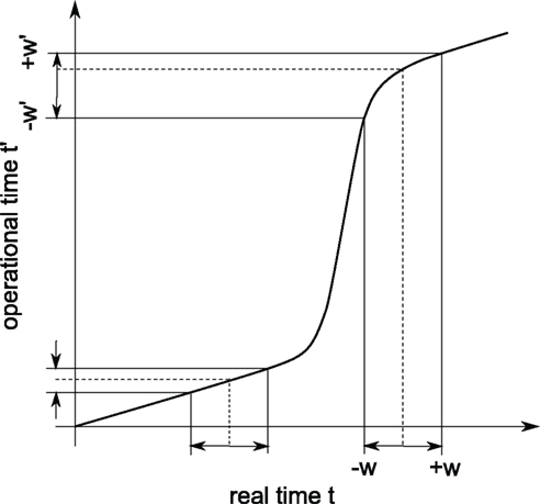
Figure 1. Illustration of the conversion from real (horizontal) to operational (vertical) time. The thick curve shows a cumulative rate profile, which serves for the transformation from real time to operational time. The dashed lines indicate the positions of two example spikes prior to dithering. A constant dither window ±w in real time is converted to non-constant dither windows ±w′ in operational time.

FIGURE 2

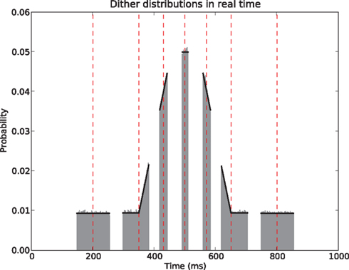
Figure 2. Uniform dithering in operational time. Real time distributions of dithers at selected points (red vertical dashed lines) in the time course of the rate. For each time point an identical uniform, fixed width dither of w′ = ±30 ms in operational time was used. The dither distributions (gray, bin width 5 ms) at each original spike position are obtained empirically by 100000 dither repetitions of each spike. The rate profile used for the mapping is shown in black.

A fixed range in operational time may constitute an interesting surrogate generation method, as it preserves the estimated rate profile exactly, and has an intuitive interpretation: in order to stand out from the noise, spike synchrony needs to be more precise in regions of high rate requiring only a smaller dither for effective destruction. However, if we fix the dithering boundaries in real time, to ±w, say, this produces a dithering distribution following the rate profile as shown in Eq. 8, with mapped boundaries [t − w,t + w], meaning

Non-uniform dithering distribution

Following Gerstein’s (2004) use of the square root function to scale in the dithering, we allow here for a general dithering distribution shaped according to a composition of the rate profile. Using Eqs. 9 and 3 with a time dependent dithering distribution, a general dithering method following a function of the local rate profile would map this rate according to

The question now becomes: how well is λ(t) preserved, depending on the choice of g. Below we show how the two obvious choices, g(x) = 1/2w (uniform dither in real time) and g(x) = x (uniform dither in operational time with fixed range in real time), both affect λ(t) in negative but opposite ways. For this we allude to Jensen’s inequality (Gradshteyn and Ryzhik, 2000) which in the continuous case states that if φ is a convex function, then

It is straightforward to show that for λ convex on the interval [y − w,y + w] the above yields

while the converse holds for a concave λ. Starting with UD [g(x) = 1/2w] and assuming a locally convex profile, combining Eqs. 10 and 12 gives

where λ_D(t) can be interpreted as the “dithered” rate profile. Thus surrogates generated by UD have an increase in rate in convex regions of the profile, and conversely a decrease in concave regions, relative to the original rate profile. As expected, this is equivalent to a smoothing of the original profile (see Figure 4). For the case in which the dithering distribution follows the rate profile itself (g(x) = x), we obtain

The effect here is the opposite to that of UD; λ_D(t) now exaggerates the non-stationarities, decreasing in convex regions and increasing in concave ones, relative to λ(t).

Joint-ISI Dithering

A similar exaggeration of the profile was previously noted in Gerstein (2004), where the feature to be preserved is the ISI distribution. In this surrogate method, the joint-ISI distribution is constructed from pairs of successive intervals (see Figure 3). Each spike is situated on the joint-ISI surface according to its pre- and post-intervals and moving a spike is equivalent to displacing the point along the perpendicular to the main diagonal in the joint-ISI plot. The surrogate method is then based on dithering the spikes following the local joint-ISI distribution, in the same way as dithering following the rate profile.

FIGURE 3

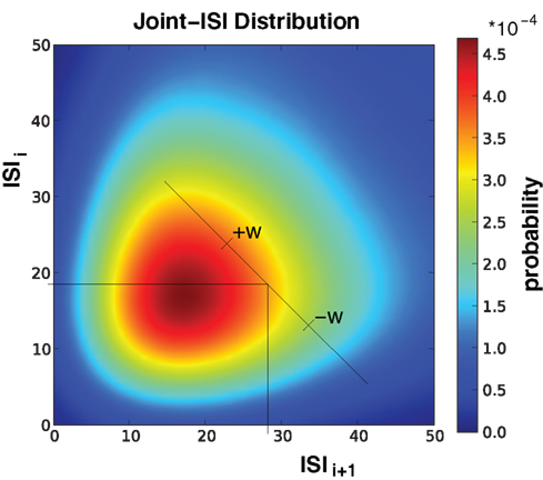
Figure 3. Illustration of Joint-ISI dithering. Joint-ISI distribution obtained from 1000 spike train realizations (same parameters as in Figure 4). The two perpendicular lines mark one particular spike with a particular ISI relative to its preceding (ISI_i) and its following spike (ISI_i+1). The spike is dithered within the interval [−w, +w] according to the non-uniform probability given by the joint-ISI distribution (color coded).

Gerstein (2004) observed that the peakedness (kurtosis) of the ISI distribution of the resulting surrogates is increased relative to the original shape; meaning the surrogate spike trains are more regular in their activity than the original. We now understand that this occurs as result of Eq. 14; each of the perpendicular cuts of the joint-ISI distribution sees its shape emphasized increasing the peakedness of the two-dimensional distribution. Consequently the shape of the marginal ISI distribution is also emphasized.

To overcome this effect Gerstein (2004) proposes to take the square root of the joint-ISI distribution before applying the dithering procedure. The surrogates then exhibit an ISI distribution very close to the original for dither widths on the order of 10 ms. Setting in Eq. 10 does not lead to λ_D(t) = λ(t), however its smoothing property counterbalances the emphasizing property of the profile itself, providing a significant improvement as can be seen in Figure 4.

FIGURE 4

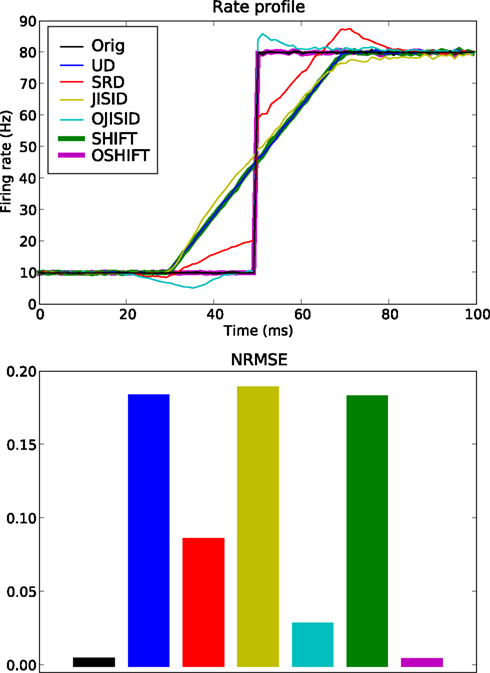
Figure 4. Conservation of rate profile at ±20 ms dither width. A total of 5 × 10⁵ trials are used, with an underlying rate following the black curve in the top panel. The estimated rate profiles (top panel) yielded by the surrogate methods are shown in color (see legend and Table 1). The lower panel shows a bar plot of the normalized root mean square error (NRMSE) of each surrogate method compared to the original PSTH (resolution 1 ms). The leftmost bar is the NRMSE of the original PSTH compared to the true rate profile.

ISI Conserving Dithers in Operational Time

Combining both, the ideas of operational time for rate conservation and joint-ISI based dithering for interval conservation, we propose a novel surrogate method. It consists in first mapping the spikes to operational time, then applying a joint-ISI based dithering in operational time with real time fixed boundaries, before finally mapping the spikes back to real time.

The dithering of the whole spike train (Pipa et al., 2008), that is adding a single uniformly distributed shift to all spikes, can also be applied in operational time. If the process is a renewal process in operational time, then such a surrogate constitutes an ideal surrogate, as it conserves both the ISI and rate features of the real time process. However the dithering ranges varies depending on the position of the individual spikes relative to the rate profile.

We show that both methods conserve the spike rate as well as the ISI distribution.

Simulation Methods

Spike dithering is now widely used in the detection of excess synchrony in parallel spike trains and the investigation of patterns and temporal coding. However its exact effect on the statistics of the spike trains has not been studied in detail.

An analysis is only useful for the experimentalist if it is based on biologically realistic rate profiles and ISI distributions. Due to the restricted power of our present theoretical tools an appropriate level of realism is only achievable by computer simulation. Fortunately, the progress in computer hardware and methods for trivial parallelization in high-level programming languages has now considerably expanded our capabilities compared to the time when dithering was first considered. The algorithms described below are implemented in Python (Langtangen, 2006) and executed in parallel using the techniques described in Denker et al. (2010). Example code for implementing dithering in operational time is available at www.spiketrain-analysis.org.

It is intuitively clear that spike dithering works for a Poisson process with a constant intensity in the dithering interval (see Diesmann et al., 2009 for a thorough introduction). Thus as soon as the spike train exhibits temporal structure such as refractory periods, dithering may be questionable. In addition, the question of the adequate choice of dithering width needs to be addressed. If the width is kept too small compared to the tolerated jitter in synchrony, the sensitivity of the detection may be affected (Pazienti et al., 2008). For excess synchrony detection, the dither width clearly depends on both the hypothesis being tested for (the allowed jitter) and the requirement to conserve the firing rate profile.

In the following sections we compare the different surrogate methods listed in Table 1 in two steps. In the first step we examine the methods’ ability to preserve the rate profile of the spike trains as well as their ISI distribution. Both are primary features of spike trains which ought to be conserved adequately. In the second step we quantify how the potential non-preservation of these features impacts spike correlation analysis, using coincidences as an example, and may lead to erroneous conclusions on the spike correlation structure of the data.

Table 1

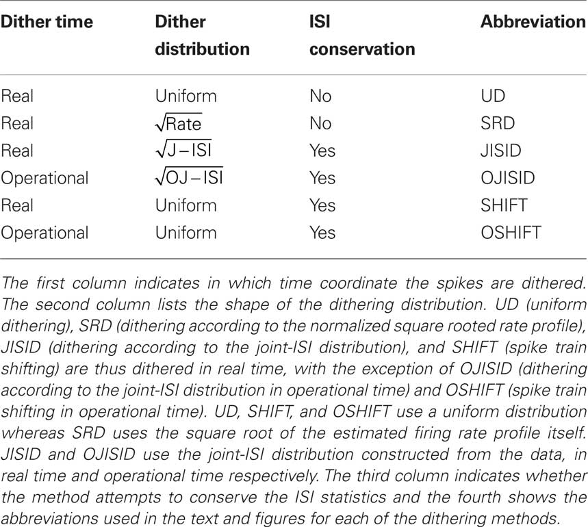
Table 1. The investigated dither methods and their features.

Benchmark Data

In order to compare the different surrogate methods, we simulate continuous time spike trains exhibiting both rate non-stationarities and non-Poisson ISI statistics. The standard rate profile used is shown by the black curve in Figure 4 consisting of a single step, with a base rate of 10 Hz. In our study we parameterize the profile by the size of the step Δλ. In the FP and FN analysis below we use 50 trials and restrict Δλ to the range between 0 and 100 Hz, leading to an upper firing rate of at most 110 Hz.

The duration of 100 ms corresponds to the typical length of the analysis window in time-resolved correlation analysis (Grün, 2009). The individual trials are produced by mapping a unit rate gamma process (renewal process with gamma distributed ISIs and rate 1 Hz) through the inverse function of the integrated rate profile (τ⁻¹ above) to real time. In other words a time rescaled stationary process. The spiking regularity is thereby defined through the shape parameter of the gamma process in operational time γ_op or alternatively its coefficient of variation CV_op, which due to the deterministic mapping leads to a constant CV = CV_op in real time. The resulting spike trains exhibit non-stationary firing rates and a non-trivial total ISI statistics.

Implementation of Dithering Methods

In the order of Table 1, we start with UD in real time. As explained in the previous sections, we implement UD by adding a random number drawn from the uniform distribution U(−w,w) independently to each spike time in the spike train. Next for the rate profile dependent method SRD, we first estimate the firing rate profile through the peristimulus time histogram (PSTH) constructed over the trials on a 1-ms resolution. The amount of smoothing applied depends on the number of trials; for 50 trials we choose a 10-ms Gaussian smoothing. From this smoothed PSTH we construct a linearly interpolated function to provide us with a continuous rate profile λ(t). Then each spike t_i is dithered according to the normalized segment of the exponentiated rate profile: t_i → s_i where for t∈[t_i−w, t_i + w] and 0 otherwise. SRD uses β = 0.5.

The SHIFT surrogate is constructed simply by adding the same random number drawn from the uniform distribution U(−w,w) to each spike time in the spike train. Thus UD and SHIFT constitute the limits of the pattern-jittering method proposed by Harrison and Geman (2009). In broad terms, this method fixes a threshold for the ISIs of interest. ISIs larger than this threshold allow for a segmentation of the data into patterns, which are dithered independently (the same random number is added to each spike of a pattern). In UD, the patterns are individual spikes and thus the ISI threshold is at 0, leading to a maximal perturbation of the ISI distribution. In SHIFT, the whole spike train is a single pattern and the ISI threshold is larger than the largest ISI, leading to a minimal variability. Observing the performance of these two limiting methods will give us an idea on where to situate pattern-jittering, with respect to other methods. We also extend SHIFT to an operational time version OSHIFT, which dithers the whole spike train in operational time. The mapping is done through the integrated PSTH. The real time dither range is thus no longer fixed.

For the ISI dependent methods, JISID and OJISID, we first construct the JISI matrix on a 1-ms resolution (in real and rescaled operational time respectively). The size I_max of this matrix was set to 100 ms × 100 ms. In general, the choice of I_max will depend on the mean and standard deviation of the ISI distribution. Once filled, the matrix is square rooted (Gerstein, 2004). In the case of a small number of trials, the matrix is additionally smoothed with a 2D Gaussian of width 3 ms. From this square rooted matrix we proceed to construct a 2D interpolated function J(x,y) through bilinear interpolation (Press et al., 2007), where 0 < x,y ≤ I_max are the pre- and post-inter-spike intervals respectively. The dithered position of a spike t_i with pre- and post-intervals x_i and y_i is then given by t_i → t_i + z_i with for 0 < x_i + t,y_i − t ≤ I_max and 0 otherwise. The spikes are dithered in parallel; that is the dither distribution is initially fixed for each spike at the beginning of procedure, based on the position of neighboring spikes. It may seem like a dynamic version, in which one first dithers (assuming the spikes are numbered) even spikes, then updates the joint-ISI coordinates before dithering the odd spikes, would be more accurate. However the conservation properties and the excess synchrony detection performance remain unaffected. The same procedure is used in the OJISID method once the spike trains were mapped to operational time. The joint-JISI matrix is then constructed in operational time. To make the matrix sizes compatible between the two methods we scaled the operational time back down to a duration of 100 ms, relative to a bin size of 1 ms. Spikes which fall out of the matrix are dithered uniformly within the initial dither width.

Quantification of Feature Conservation

In order to have a reliable comparison of feature conservation across the surrogate methods, we simulate a total of 5 × 10⁵ trials following the procedure outlined above. Except for UD and SHIFT which are independent of the rate profile, all methods make use of all the trials in estimating the rate profile and the JISI distribution. We then calculate the normalized root mean square error (NRMSE) of the surrogate PSTH obtained from all surrogate trials H_s with respect to the true PSTH obtained from the original trials H_T at a resolution of 1 ms as , where and are the maximum and the minimum spike count in the histogram of the original spike trains respectively and N is the number of bins of the histograms.

The NRMSE is also calculated for the respective ISI distributions (1 ms resolution) in a similar fashion, quantifying the destruction of the original ISI statistics.

False Positive and False Negative Evaluation in Correlation Analysis

Feature conservation is only part of the assessment of a surrogate method. It may indicate its flaws and advantages, however it does not guarantee that it will be useful in the context of a specific analysis of the data. Here we concentrate on the example of spike correlation analysis, and show how surrogates can be used for testing for the presence or absence of correlation between spike trains and for deriving their significance. In the correlation analysis we are interested to detect the presence or not of excess precise spike synchrony, beyond that explained by the firing rate and the ISI statistics. We define a synchronous event by two spikes (one from each neuron) occurring within ±1 ms of each other. Surrogates serve as an implementation of the null-hypothesis of independent firing. By dithering the precise relationship of the spikes of the two spike trains is destroyed.

To evaluate the performance of the surrogates in the context of correlation analysis we look at FP rates in data containing no excess synchrony and FN rates in data containing excess synchrony. In the statistical analysis we are here following the terminology of Ventura et al. (2005). For each parameter configuration and surrogate method, the FP and FN rates are obtained as follows. We begin by generating 1000 data sets with the same parameter configuration. A data set consists of 50 trials (100 ms duration) of two parallel spike trains generated according to a defined rate profile and interval statistics as in the study of feature conservation estimation of single spike trains. In case of studying the FN rate, the parallel spike trains contain correlated spiking due to insertion of jittered (±1 ms) coincident spike events at rate λ_c. For the FP analysis, the insertion is omitted and the spike trains are independent on a fine temporal scale, but are correlated on a slower time scale due to correlated (identical) rate profiles.

For each data set, we produce 1000 surrogate versions. Each set of surrogates is analyzed as the original data set for the occurrences of coincident spike events. In each data set, the number of coincidences of an allowed temporal precision (here ± 1 ms) is counted. A coincidence is detected by testing if there is one spike (or more) of the second spike train within ±1 ms relative to a spike of the first (reference) spike train. If more spikes occur within an individual coincidence window, this is counted as one coincidence (“clipping”). From the coincidence counts derived from the surrogates we construct the surrogate coincidence count distribution, which serves to estimate the significance of the coincidence count of the original data by calculating the p-value.

Thus for one parameter configuration of the data and surrogate method, we obtain 1000 p-values (p_i for i = 1,…,1000). Given a significance level α, which we fix to 0.01 in the following, we convert these results into counts of positive (significant) results, i.e., N₊ = Σ_iφ(p_i ≤ α), and counts of negative (non-significant) results, i.e., N₋ = Σ_iφ(p_i > α), where φ(x) = 1|0 if x is true|false. If the chosen parameter configuration involves injected synchrony, then the FN rate in percentage is given by 100 · N₋/N (where N = N₊ + N₋ = 1000), i.e., the percentage of falsely undetected correlation. Conversely, if the parameter configuration does not involve injections, then the FP rate reads 100· N₊/N indicating the percentage of falsely detected correlation (Louis et al., 2010).

In general the FP rate (empirical type I error) does not coincide with the prespecified significance level α because the surrogate distribution only imperfectly resembles the distribution of coincidence counts of independent data. If the independent distribution is known a matched significance level α_m can be determined which restricts the FP rate to a prespecified value. However, with knowledge of the independent distribution, typically no surrogate method is required in the first place. The FN rate (empirical type II error) can be used to compare the sensitivity or test power of different surrogate methods if they are adjusted to produce the same FP rate. Differences in sensitivity may then, for example, originate from a different effectiveness of the surrogate methods in destroying injected coincidences.

Calibration Based on Simulated Data

Effect of Dither Surrogates on Rate Profile

We compare a total of six surrogate methods (UD, SRD, SHIFT, OSHIFT, JISID, and OJISID, listed in Table 1) in their ability to preserve the underlying rate profile. The dither width was fixed at 20 ms; intentionally large such as to accentuate the differences between methods. The parameters of the profile are Δλ = 70 Hz and γ_op = 3 (Figure 4).

We observe that the UD, SHIFT, and JISID methods perform worse (highest NRMSE), systematically deviating away from the rate in the vicinity of the step. The effect is intuitive for UD and SHIFT which lead to a smoothed profile, corresponding to a convolution as shown in Eq. 13. In the case of JISID, the effect can be understood by considering the likely positions of the interval borders in the JISI matrix given by the previous and the next spike in dependence of the rate profile. When the rate is increasing, as is the case at the step, the post-interval is likely to be smaller than the pre-interval, thus the JISI based dither will tend to recenter the spike and shift it back in time. Repeating this effect over trials leads to a systematic shift of the rate profile. The rate would be shifted in the other direction in downward transients.

Taking the square root of the profile as a dithering distribution more than halves the NRMSE, as can be seen from the performance of SRD. OJISID performs even better, apart from the slight emphasizing effect at the step, which was anticipated in Eq. 14. Finally OSHIFT is at the level of the variability in the original PSTH as it does not modify any of the statistics of the processes.

Effect of Dither Surrogates on ISI Distributions

The same set of trials as in the previous section is then used to assess the conservation of the ISI distribution (Figure 5). The UD and SRD methods deviate most from the original distribution, showing the largest NRMSEs (computed for the surrogate distributions compared to the distribution of the original trials). Next we find the JISI method, which conserves the distribution far better. It is still quite far from the original distribution, which we attribute to the size of the dither window, which is larger than the width of the distribution. The method conserves the ISI distribution with much higher precision for dither widths on the order of 10 ms (not shown, see Gerstein, 2004). As anticipated, the OJISI method not only preserves the rate profile, it also yields surrogates with an ISI distribution even closer to the original, as can be seen from the reduced NRMSE.

FIGURE 5

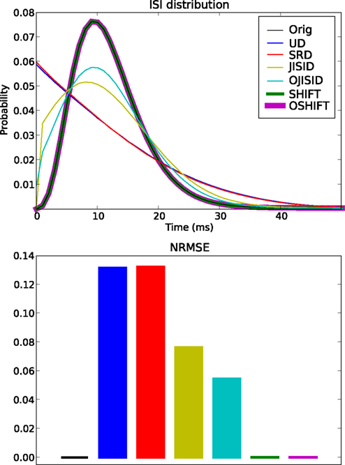
Figure 5. Conservation of the ISI distribution at ±20 ms dither width. The top panel shows the original and estimated ISI distributions based on the various surrogates (colors, see legend). The original ISI distribution curve is covered both by SHIFT and OSHIFT traces. The lower panel shows a bar plot of the NRMSE performances of each surrogate method (colors as in top panel) compared to the ISI distribution of the original spike trains. The heights of the bars for SHIFT, OSHIFT and the NRMSE of the ISI distribution of the original spike trains compared to the true distribution (black) are amplified just to indicate that the NRMSE was computed for all cases. The data are the same as shown in Figure 4.

However the most accurate methods are the SHIFT and OSHIFT methods, as expected. They perfectly conserve the ISI statistics of the processes. For SHIFT, this is obvious. For OSHIFT, the ISI statistics of the process in operational time are perfectly conserved, so applying exactly the same mapping to and from operational time leads to a perfect conservation in real time. However the ISI sequence of a single trial is modified, unlike in the SHIFT method.

Combining the last two results, we can safely conclude that the OSHIFT and OJISID methods are by far the most feature preserving surrogate methods amongst the six being compared.

Effect of Dither Surrogates on Sensitivity of Correlation Analysis

To see how the methods compare in the context of correlation analysis, we devised two separate analyses focusing on different parameters. The first analysis evaluates the dependence of FPs and FNs on the strength Δλ of the non-stationarity in rate (Figure 6). In the second analysis Δλ is set to 70 Hz and we investigate the dependence of FP and FN results on the coefficient of variation (CV) controlled by the shape parameter γ_op of the process (Figure 8). The task of the surrogates is to detect the presence of excess spike synchrony (±1 ms), beyond that explained by the firing rate and the ISI statistics. We set the dither range in the various surrogate methods to ±20 ms throughout this part of the study for the intended destruction of the precise temporal relationship between the spikes of the two neurons. This dither range is a lower bound for OSHIFT; spikes may be dithered by larger amounts in the low rate region. In addition, Figure 7 shows a scenario where for the first analysis we progressively reduce the dither width of UD.

FIGURE 6

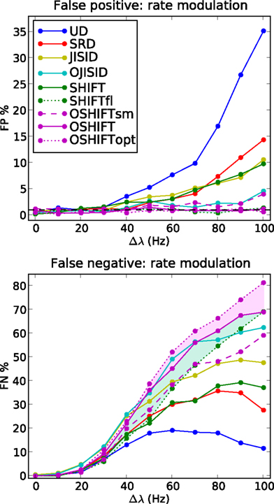
Figure 6. FP and FN percentages as a function of the step amplitude Δλ, with fixed γ_op = 3. SHIFTfl is the SHIFT surrogate applied to a stationary process with the average spike rate of the rate step scenario. OSHIFTsm is a version of OSHIFT where the mapping to operational time constructed from the data is smoothed (10 ms Gaussian). OSHIFTopt is based on the true rate profile and the injection rate for the lower plot is λ_c = 2 Hz. A worst case estimate of the standard deviation of the FP/FN percentage is given by the error in the mean , i.e., for a Bernoulli process with p = 0.5 and n = 1000 realizations as used here.

FIGURE 7

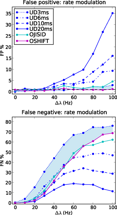
Figure 7. Comparison of sensitivity at matched false positive rates. FP and FN rates as a function of the rate step amplitude, for varying dither widths of UD. Other parameters as in Figure 6

FIGURE 8

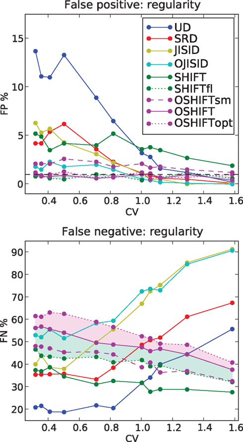
Figure 8. FP and FN percentages as a function of the regularity of the processes. The firing rates of the parallel spike trains follow the step profile with Δλ = 70 Hz. The regularity of the spike trains is parameterized by the coefficient of variation CV = CV_op. FP values are shown for CV values corresponding to shape parameters γ_op = 10,8,6,4,2,1.5,1,0.9,0.8,0.6, and 0.4 (from left to right). Each data point results from 1000 repetitions.

We begin with the rate dependence analysis (Figure 6) and clearly identify UD as the method with the highest FP rates (up to 35% for Δλ = 100 Hz) and correspondingly the lowest FN rates. Then comes the SRD method which attempts to better preserve the rate step but ignores the ISI statistics. With similar FP performances, we find SHIFT and JISID, producing FPs up to 10%. However the SHIFT method is clearly superior when looking at the FN rates which are consistently lower. Thus for the same accuracy, SHIFT is more sensitive than JISID.

The operational time methods OJISID and OSHIFT are considerably more conservative, with FP rates of at most 5%. However their level of sensitivity appears to be far lower, with high FN rates going up to 70%. In the Appendix we explain why in fact OSHIFT reaches the maximum sensitivity: The other surrogate methods are smoothing the rate profile. This leads to a distribution of coincidence counts which is shifted to a lower mean compared to the mean of the actual independent distribution. Consequently a smaller fraction of the dependent distribution is located to the left of the threshold coincidence count determined by the significance level. The FN rate appears to be reduced compared to OSHIFT but this is trivially so because the FP rate is larger than the significance level suggests. If a larger fraction of the independent distribution is to the right of the significance level also more of the dependent distribution is. The FN rates are only decisive if the FP rates are comparable.

Figure 6 shows three variants of OSHIFT: one in which the true rate profile is used (OSHIFTopt, short dashed purple), one in which the PSTH is smoothed before being used for the mapping (OSHIFTsm, long dashed purple) and one without the smoothing (OSHIFT, solid purple). An immediate observation is that smoothing the PSTH, which is initially quite variable due to the limited number of trials (50) induces a strong increase in FPs, from 0 to 5% at Δλ = 100 Hz. Thus integrating the PSTH for deriving the rate mapping provides an inherent reduction of noise and leads to a reliable mapping to and from operational time. SHIFT and JISID perturb the rate profile and exhibit the same dependence of the FP rate on Δλ. Using operational time, the FP rate of OJISI does not drop to the one of OSHIFT but reaches the level of OSHIFTsm. The reason is that the smoothing of the rate profile described above is also used in OJISI . The region shaded in light purple indicates the effect of using a PSTH instead of the true rate profile, and in some sense illustrates the distance to the optimal surrogate. Another way to explore the effect of non-stationarity in spike rate on a particular surrogate method is to compare the results for non-stationary data with the result of stationary data but otherwise similar characteristics. The curves labeled SHIFTfl (short dashed green) show the result of the SHIFT surrogate method applied to a data set generated by a stationary process parameterized by the average spike rate of the non-stationary process and identical regularity. The distance between SHIFT (solid green) and SHIFTfl (short dashed green) illustrates the cost of ignoring non-stationarity. For SHIFT the FP rate substantially increases with Δλ while it stays at the expected level for SHIFTfl. Thus, the smaller FN rate of SHIFT as compared to SHIFTfl is due to the higher FP rate of SHIFT. We find that OSHIFT (solid purple) lies between the optimal surrogate performances for non-stationary (OSHIFTopt, short dashed purple) and stationary (SHIFTfl, dashed green). The performance of OSHIFTopt and SHIFTfl is optimal in the sense that they destroy all coincidences, and have an FP rate at the expected level because the rate profiles are exactly respected. At the same FP rate no other method can have a lower FN rate. The rate of injected coincidences λ_c is stationary and the same in both cases. Therefore, in the data set with a rate step (OSHIFTopt) the distance between the number of coincidences in the data and the expected number of coincidences in the surrogates is smaller (see also Grün et al., 2003). This leads to the larger FN rate of OSHIFTopt compared to SHIFTfl illustrated by the conjunction of the light blue and light purple areas. The region shaded in light blue indicates that the increase in the FN rate (light blue) of OSHIFT compared to the stationary setting (SHIFTfl) is about half of the optimal value (conjunction of light blue and light purple) due to the remaining noise in the estimation of the integrated rate profile.

To illustrate the superiority of the operational time methods, we performed the same analysis using UD with reducing dither widths ±20, ±10, ±6, and ±3 ms. The results are shown in Figure 7. We observe that by the time the FP rates are brought down to the level of OJISID (still larger than OSHIFT: upper panel, light blue area) by using a dither width of ±3 ms, the UD method is far less sensitive than OSHIFT or OJISID (lower panel, light blue shaded area). This signifies that one cannot reach the level of performance of the more advanced methods proposed in this study by simply reducing the dither width of simpler methods. The Appendix shows that the loss of sensitivity of UD with decreasing dither width is due to an insufficient destruction of the injected coincidences.

The second parameter which we investigate is the spiking regularity, quantified by the shape parameter of the ISI (gamma) distribution in operational time γ_op (see Figure 8). More precisely we plot the FP and FN rates as a function of the coefficient of variation . As in Figure 5 we set Δλ = 70 Hz.

For CV > 1, we find that most methods, except SHIFT, are operating at reasonable FP rates. However, once the processes become more regular than Poisson, UD shows a strong increase in FP rates. The performance of SHIFT does not seem to depend too strongly on CV and the offset of a few percent above the significance level is due to the smoothing of the rate profile, as can be seen from the SHIFTfl curve. SRD and JISID show a fairly similar behavior, reaching 5% FP rates for highly regular processes, on par with SHIFT. Again, JISID is above the significance level as it shows poor rate conservation properties. Below we find the operational time methods, of which OSHIFT lies at the significance level, unaffected by the increasing regularity.

Turning to the FN rates (Figure 8, lower panel), we note that UD and SRD follow a similar trend, opposite to their FP rate trend. SHIFT proves to be fairly sensitive through the parameter range and shows again an upward slope with regularity. In contrast, JISID and OJISID become more sensitive as regularity increases. The reason for this increased FN rate in irregular regimes is that most spikes have small pre- and post-intervals (burst) and thus cannot be dithered by large enough amounts, relative to the coincidence width (±1 ms). The OSHIFT method looses in sensitivity as the process gains in regularity, maintaining its distance with the optimal surrogate for the non-stationary (light purple shading) and stationary (light green shading) cases. This suggests that as in Figure 6 its performance is limited by the accuracy of the mapping to operational time.

Combining the observations made above, we conclude that OSHIFT is the most conservative method, and in terms of sensitivity, for a fixed accuracy, is the closest to optimum. The OJISID also outperforms simpler methods, however the constraints on the dither range by the previous spike and the next spike limits variability of the coincidence counts in the surrogates and its implementation is far more involved.

Application to Experimental Data

To assess the behavior of the various surrogates in an experimental setting, we consider a pair of neurons recorded non-simultaneously in the primary visual cortex of the anesthetized macaque monkey (Aronov et al., 2003). The reason for choosing non-simultaneous recordings is that we need to be in a situation in which we can be certain that there is no excess synchrony; only then can we be sure that we are observing FP results. The stimuli are transient presentations of stationary gratings of varying spatial phase. Each neuron was recorded from in different sessions and with a different stimulus presented. A total of 64 trials were obtained for each neuron; the responses are shown in Figure 9. As one can see from the dot display and the PSTH, both neurons exhibit strong rate transients within the analysis window of duration 100 ms covering the time interval [250, 350 ms]. The spike rates of the two neurons peak at 200 and 250 Hz, respectively, with highly regular spike sequences.

FIGURE 9

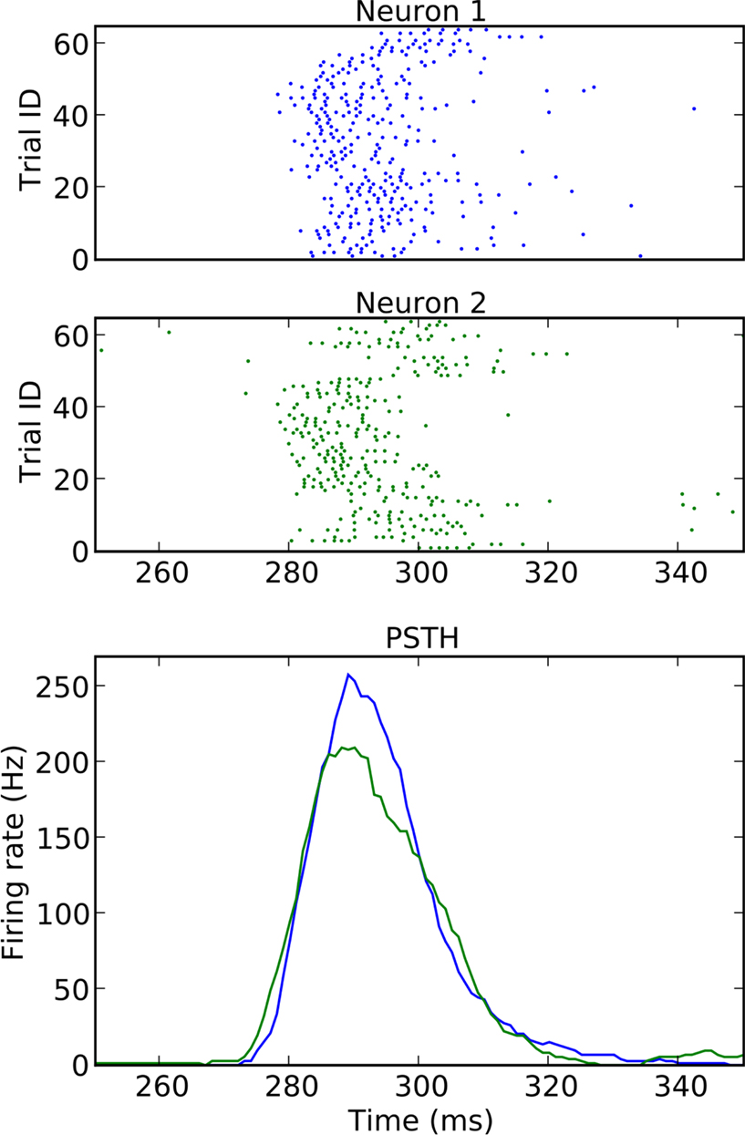
Figure 9. Dot displays (upper panels) and smoothed PSTHs (bottom panel) of two simple cells recorded from monkey primary visual cortex recorded in the same session, however under different stimulus conditions. The stimuli for the two neurons are stationary transient gratings of different orientation. The data are described in (Aronov et al., 2003) and publicly available at neurodatabase.org. Neuron 1 corresponds to file 410106s in condition 5, and neuron 2 to file 410106t in condition 1.

We treat these two neurons as if they were simultaneously recorded and test for excess coincidences with an allowed jitter of ±1 ms. Due to the large amplitude of the transient we use a dither width of 10 ms for all methods except OSHIFT, which applies a non-uniform dither with a range in real time of at least 10 ms. For each surrogate method we generate 10000 surrogate versions of the recordings from the neuron with the mildest rate transient. The resulting coincidence distributions and p-values of the observed coincidence count (black line) are shown in Figure 10.

FIGURE 10

Figure 10. Surrogate coincidence distributions based on experimental data shown in Figure 9, with a dither width set to 10 ms in range-bounded methods. The vertical black line indicates the coincidence count in the original data.

The resulting surrogate distributions are compatible with the observations made in the previous section on synthetic data. The non-ISI conserving methods, UD and SRD, would detect a significant (above 1% level) number of coincidences (p-value below 10^–3 in both cases). SHIFT does not detect significant excess synchrony. In turn, the more conservative methods, JISID, OJISID, and OSHIFT clearly do not observe any excess synchrony, as one would expect from independent recordings.

Thus in such strong rate transient regimes, we recommend the use of more advanced methods which take into account the observed rate and ISI properties of the recordings. The example data exhibit considerable cross-trial non-stationarity. Nevertheless OSHIFT is sufficiently robust and remains the method of choice.

Alternatively, one can reduce the dither width of more basic methods, however this will induce a substantial reduction in sensitivity, for a similar accuracy, as shown in Figure 7.

Discussion

The result of our study of the family of surrogate methods based on dithering is that the methods considering the ISI distribution behave best with respect to rate modulations and regularity of the spike trains. The novel techniques of joint-ISI dithering (OJISID) and train dithering (OSHIFT) in operational time are the most robust methods, since they exhibit the lowest FP rates amongst the surrogate methods considered in the paper. The apparently lower FN rate of other methods is a direct consequence of the increased FP rate. At the same FP rate, simpler methods cannot match the sensitivity of OSHIFT and OJISID. Thus this surrogate approach should be restricted to the application to Poisson spike trains with small rate fluctuations. This is also illustrated by the analysis of the macaque V1 recordings considered above. Even though the neurons were recorded in different sessions and are expected not to exhibit excess synchrony, UD does consider the empirical coincidence count as highly significant.

In the Appendix we explore the theoretical relationship between FP and FN by assuming that the true independent and dependent distributions of coincidence counts are known. In this scenario the significance level used for a particular surrogate method can be adjusted to generate a desired FP rate. As a consequence all surrogate methods which effectively destroy coincidences also produce identical FN rates. Methods which leave a fraction of the coincidences intact have a lower sensitivity.

The spike exchange (Smith and Kohn, 2008; Grün, 2009) surrogate methods may seem to have an advantage over the methods covered in this study, as they conserve the PSTH exactly, account for non-stationarities across trials and keep the spike count per trial constant. Thus we expect that they perform better than UD or SRD. However they do not attempt to conserve ISI distribution and as we demonstrated in the FP rate analysis, high firing rates combined with spiking regularity place strict requirements on the surrogate method.

Having considered the limiting cases (UD and SHIFT) of the pattern-jitter method (Harrison and Geman, 2009), we believe that their performances situate the performance of the latter. We anticipate that pattern-jitter will not represent an improvement over OSHIFT for the processes considered in this study. However further studies including cross-trial non-stationarities are required to clearly differentiate the methods and define the conditions under which they are most applicable.

Experimentally recorded spike trains have the added complication that they not only exhibit rate non-stationarities but also non-stationarities in the CV (regularity) of the ISIs within trials (Shinomoto et al., 2003, 2009; Davies et al., 2006; Nawrot et al., 2008; Kilavik et al., 2009). In consequence single trials may have a rate profile and a potentially independent regularity profile. It remains to be investigated whether a concept similar to operational time for converting a non-stationary rate process to a stationary one, can be found to account for regularity non-stationarities. Again surrogate generation methods need to be thoroughly tested for processes that are non-stationary in both parameters.

In a given application it may be of interest to not only include the rate profiles and the interval statistics but also additional features like a baseline spike correlation into the null-hypothesis. Whether it is possible to limit the destructive power of dithering to achieve this needs to be investigated.

The comparison between the joint-ISI dithering methods in real and operational time highlights that given a non-stationary rate the ISI distribution is in a formal sense not defined. The long intervals in the ISI distribution in real time are dominated by contributions from the low rate regimes. Nevertheless, the full distribution is used to dither spikes also in high rate regions where short intervals dominate. The role of the transformation to operational time is to get access to a well defined ISI distribution valid at any point on the temporal axis. Nawrot et al. (2008) exploited the same idea to reliably assess the CV of ISIs in neuronal data.

Our theoretical framework explains why the square root profile introduced by Gerstein (2004) is superior to a flat dither profile and to the profile following the original distribution. We have no evidence, however, in what sense 0.5 is an optimal choice of the exponent. In fact, it seems that for an arbitrary rate profile an exponent with an improved performance can be found (not shown). This raises the intriguing question whether there is a locally optimized time dependent choice of the exponent β(t).

The method of dithering in operational time emphasizes the dual role of the size of the sliding analysis window in time-resolved correlation analysis. The original paper on the Unitary Events analysis (Grün et al., 2002b) states the two characteristics controlled by the parameter: (1) The window needs to be narrow enough to assume stationarity of the rate. (2) The window size needs to be large enough to collect sufficient statistics but adapted to a potentially temporally constrained occurrence (“hot region”) of correlation. With reliable surrogate methods at hand to construct the distribution of coincidence counts for non-stationary rate profiles, the first condition can be relaxed and the experimenter has more freedom to optimize for the dynamics of correlation.

The use of the firing rate profile for a coordinate transformation has also been emphasized in the proposal to use order statistics for spike train resampling (Richmond, 2009). The method allows for the generation of surrogate spike trains with constrained spike numbers and a specified rate profile. Rooted in the theory of order statistics it constitutes a model in itself. However the effects of spiking regularity are so far neglected. It is of interest to find the relation between this method and different versions of dithering, as they have the same aim.

It has been argued that brain processing may be reflected in the higher-order correlation of multiple parallel spike trains (Gerstein et al., 1978; Abeles, 1991). The analysis in this paper, however, is restricted to two parallel processes. Future work needs to investigate whether the idea to work in a transformed temporal coordinate can be extended to higher dimensions. This is relevant because it is conceivable that in higher-order analysis perturbations of assumed surrogate invariants like rate profile and interval statistics may become more problematic.

We have studied a particular injection model where the rate of coincidence is constant while the overall spike rate is changing. This naturally leads to an increase of FN with increasing spike rate. An alternative model would be one where the rate of injected synchrony increases with the spike rate. In this sense our model is a worst case scenario for the detection of synchrony. Which model is best adapted to brain processes remains to be investigated.

While the struggle to construct sensitive and robust surrogates for neuronal spike data continues, we have presented some practical and conceptual advances. On the basis of our study we recommend not to hesitate to exploit the computer technology available today and to use surrogate methods based on operational time to simultaneously conserve the rate profile and the ISI distribution.

Conflict of Interest Statement

The authors declare that the research was conducted in the absence of any commercial or financial relationships that could be construed as a potential conflict of interest.

Acknowledgments

The initial part of this work was conducted when S. Grün and M. Diesmann enjoyed a scientific stay with G. Gerstein in Philadelphia in May 2008. We acknowledge fruitful and encouraging discussions with the participants of the EPSRC funded “Spatio-temporal Patterns and Synfire Chains” workshop in August 2008 organized by S. Baker in Newcastle. We also thank J. Ito for useful suggestions. Partially funded by DIP F1.2, Helmholtz Alliance on Systems Biology (Germany), Next-Generation Supercomputer Project of MEXT (Japan), BMBF Grant 01GQ0420 to BCCN Freiburg, and EU Grant 15879 (FACETS). Experimental data used in this study were delivered via neurodatabase.org – a neuroinformatics resource funded by the Human Brain Project.

References

Abeles, M. (1991). Corticonics: Neural Circuits of the Cerebral Cortex, 1st Edn. Cambridge: Cambridge University Press.

Abeles, M., and Gat, I. (2001). Detecting precise firing sequences in experimental data. J. Neurosci. Methods 107, 141–154.

Pubmed Abstract | Pubmed Full Text | CrossRef Full Text

Aronov, D., Reich, D., Mechler, F., and Victor, J. (2003). Neural coding of spatial phase in v1 of the macaque monkey. J. Neurophysiol. 89, 3304–3327.

Pubmed Abstract | Pubmed Full Text | CrossRef Full Text

Beck, C., and Schlögl, F. (eds)(1995). “Transfer operator methods (chapter 17),” in Thermodynamics of Chaotic Systems. Springer Series in Computational Neuroscience (Cambridge, England: Cambridge University Press), 190–203.

Brown, E., Barbieri, R., Ventura, V., Kass, R., and Frank, L. (2001). The time-rescaling theorem and its application to neural spike train data analysis. Neural Comput. 14, 325–346.

CrossRef Full Text

Cox, D., and Isham, V. (1980). Point Processes. Monographs on Applied Probability and Statistics. Boca Raton: Chapman and Hall.

Date, A., Bienenstock, E., and Geman, S. (1998). On the Temporal Resolution of Neural Activity. Technical Report, Division of Applied Mathematics, Brown University.

Davies, R., Gerstein, G., and Baker, S. (2006). Measurement of time-dependent changes in the irregularity of neural spiking. J. Neurosci. 96, 906–918.

Denker, M., Wiebelt, B., Fliegner, D., Diesmann, M., and Morrison, A. (2010). “Practically trivial parallel data processing in a neuroscience laboratory,” in Analysis of Parallel Spike Trains, Springer Series in Computational Neuroscience, S. Grün, and S. Rotter, (New York: Springer), 416–436.

Diesmann, M., Louis, S., Grün, S., and Gerstein, G. (2009). “Spike train surrogates based on dithering in operational time,” in Proceedings of 57th Session of the International Statistical Institute, Durban, South Africa.

Gerstein, G. L. (2004). Searching for significance in spatio-temporal firing patterns. Acta Neurobiol. Exp. (Wars) 64, 203–207 (review).

Pubmed Abstract | Pubmed Full Text

Gerstein, G., and Perkel, D. (1972). Mutual temporal relationships among neuronal spike trains. Statistical techniques for display and analysis. Biophys. J. 12, 453–473.

Pubmed Abstract | Pubmed Full Text | CrossRef Full Text

Gerstein, G., Perkel, D., and Subramanian, K. (1978). Identification of functionally related neural assemblies. Brain Res. 140, 43–62.

Pubmed Abstract | Pubmed Full Text | CrossRef Full Text

Gradshteyn, I., and Ryzhik, I. (2000). Tables of Integrals, Series, and Products, 6th Edn. San Diego, CA: Academic Press.

Grimaldi, R. P. (2003). Discrete and Combinatorial Mathematics: An Applied Introduction, 5th Edn. Reading, Massachusetts: Addison Wesley.

Grün, S. (2009). Data-driven significance estimation of precise spike correlation. J. Neurophysiol. 101, 1126–1140 (invited review).

Pubmed Abstract | Pubmed Full Text | CrossRef Full Text

Grün, S., Diesmann, M., and Aertsen, A. (2002a). ‘Unitary Events’ in multiple single-neuron spiking activity. I. Detection and significance. Neural Comput. 14, 43–80.

CrossRef Full Text

Grün, S., Diesmann, M., and Aertsen, A. (2002b). ‘Unitary Events’ in multiple single-neuron spiking activity. II. Non-Stationary data. Neural Comput. 14, 81–119.

CrossRef Full Text

Grün, S., Riehle, A., and Diesmann, M. (2003). Effect of cross-trial nonstationarity on joint-spike events. Biol. Cybern. 88, 335–351.

Pubmed Abstract | Pubmed Full Text | CrossRef Full Text

Harrison, M., and Geman, S. (2009). A rate and history-preserving resampling algorithm for neural spike trains. Neural Comput. 21, 1244–1258.

Pubmed Abstract | Pubmed Full Text | CrossRef Full Text

Hatsopoulus, N., Geman, S., Amarasingham, A., and Bienenstock, E. (2003). At what time scale does the nervous system operate? Neurocomputing 52–54, 25–29.

CrossRef Full Text

Kilavik, B., Roux, S., Ponce-Alvarez, A., Confais, J., Grün, S., and Riehle, A. (2009). Long-term modifications in motor cortical dynamics induced by intensive practice. J. Neurosci. 29, 12653–12663.

Pubmed Abstract | Pubmed Full Text | CrossRef Full Text

Langtangen, H. P. (2006). Python Scripting for Computational Neuroscience, 2nd Edn. Berlin/Heidelberg/New York: Springer.

Louis, S., Borgelt, C., and Grün, S. (2010). “Selecting appropriate surrogate methods for correlation analysis,” in Analysis of Parallel Spike Trains. Springer Series in Computational Neuroscience, S. Grün, and S. Rotter, (New York: Springer), 359–382.

Nadasdy, Z., Hirase, H., Czurko, A., Csicsvari, J., and Buzsaki, G. (1999). Replay and time compression of recurring spike sequences in the hippocampus. J. Neurosci. 19, 9497–9507.

Pubmed Abstract | Pubmed Full Text

Nawrot, M. P., Boucsein, C., Rodriguez Molina, V., Riehle, A., Aertsen, A., and Rotter, S. (2008). Measurement of variability dynamics in cortical spike trains. J. Neurosci. Methods 169, 374–390.

Pubmed Abstract | Pubmed Full Text | CrossRef Full Text

Pazienti, A., Maldonado, P., Diesmann, M., and Grün, S. (2008). Effectiveness of systematic spike dithering depends on the precision of cortical synchronization. Brain Res. 1225, 39–46.

Pubmed Abstract | Pubmed Full Text | CrossRef Full Text

Perkel, D., Gerstein, G., and Moore, G. (1967). Neuronal spike trains and stochastic point processes. II. Simultaneous spike trains. Biophys. J. 7, 419–440.

Pubmed Abstract | Pubmed Full Text | CrossRef Full Text

Pipa, G., Wheeler, D., Singer, W., and Nikolic, D. (2008). Neuroxidence: reliable and efficient analysis of an excess or deficiency of joint-spike events. J. Comput. Neurosci. 25, 64–88.

Pubmed Abstract | Pubmed Full Text | CrossRef Full Text

Press, W., Teukolsky, S., Vetterling, W., and Flannery, B. (2007). Numerical Recipes 3rd Edition: The Art of Scientific Computing, 3rd Edn. Cambridge: Cambridge University Press.

Richmond, B. (2009). Stochasticity, spikes and decoding: sufficiency and utility of order statistics. Biol. Cybern. 100, 447–457.

Pubmed Abstract | Pubmed Full Text | CrossRef Full Text

Shinomoto, S., Kim, H., Shimokawa, T., Matsuno, N., Funahashi, S., Shima, K., Fujita, I., Tamura, H., Doi, T., Kawano, K., Inaba, N., Fukushima, K., Kurkin, S., Kurata, K., Taira, M., Tsutsui, K., Komatsu, H., Ogawa, T., Koida, K., Tanji, J., and Toyama, K. (2009). Relating neuronal firing patterns to functional differentiation of cerebral cortex. PLoS Comput. Biol. 7, 12591–12603. doi:10.1371/journal.pcbi.1000433.

Shinomoto, S., Shima, K., and Tanji, J. (2003). Differences in spiking patterns among cortical neurons. Neural Comput. 15, 2823–2842.

Pubmed Abstract | Pubmed Full Text | CrossRef Full Text

Shmiel, T., Drori, R., Shmiel, O., Ben-Shaul, Y., Nadasdy, Z., Shemesh, M., Teicher, M., and Abeles, M. (2006). Temporally precise cortical firing patterns are associated with distinct action segments. J. Neurophysiol. 96, 2645–2652.

Pubmed Abstract | Pubmed Full Text | CrossRef Full Text

Smith, M. A., and Kohn, A. (2008). Spatial and temporal scales of neuronal correlation in primary visual cortex. J. Neurosci. 28, 12591–12603.

Pubmed Abstract | Pubmed Full Text | CrossRef Full Text

Snyder, D., and Miller, M. (1991). Random Point Processes in Time and Space. New York: Springer Verlag.

Stark, E., and Abeles, M. (2009). Unbiased estimation of precise temporal correlations between spike trains. J. Neurosci. Methods 179, 90–100.

Pubmed Abstract | Pubmed Full Text | CrossRef Full Text

Ventura, V., Cai, C., and Kass, R. E. (2005). Statistical assessment of time-varying dependency between two neurons. J. Neurophysiol. 94, 2940–2947.

Pubmed Abstract | Pubmed Full Text | CrossRef Full Text

Appendix

The Relationship of FP and FN

In the following we compare three characteristic dithering methods (UD, SHIFT, and OSHIFT) in a situation where the FP generated by the different methods are matched by adjusting the significance level α. This cannot be done for experimental data because, as shown below, the resulting α_m depends on the detailed shape of the surrogate distribution and the calibration requires access to the true distribution of coincidence counts for independent data.

Nevertheless, the analysis of a model situation enables us to investigate the relationship between FP and FN and the limit of sensitivity. Consider a situation similar to the one discussed in Figure 6. We generate two types of data sets consisting of 100 trials of 100 ms duration of γ = 3 process realizations with a rate step at 50 ms from a base of 10 Hz to a new rate level elevated by Δλ. One type is called the correlated or dependent data set. Here we inject coincidences with a jitter of ±1 ms using a Poisson process at rate λ_c = 2 Hz and reduce the baseline rate accordingly. The second type is left uncorrelated which we call the independent data set. As in Figure 6 we vary Δλ from 0 to 100 Hz and create 10⁵ data sets for both types. Subsequently we apply the dithering methods UD, SHIFT, and OSHIFT to the data sets to generate one surrogate data set per method and original data set. Finally, for each of the methods we collocate the data into four distributions of coincidence counts: independent data, correlated data, and the corresponding two surrogate distributions. For comparison we also compile the four distributions for UD at a reduced dither width of ±3 ms.

Figure 11 verifies that at a dither width of ±20 ms the surrogate distributions for correlated and independent data are identical for all dithering methods because the dither width is large enough to destroy practically all injected coincidences. Note that in this Appendix we simplify the procedure compared to the main text in that we construct the distributions of coincidence counts by combining data from all original spike train realizations. This is less accurate because for a particular realization the surrogate distributions do not conserve the spike counts of the original data. As argued above and elsewhere (Grün, 2009) we do not recommend to do this in the analysis of experimental data but it is convenient to study the fundamental relationship between FP and FN.

FIGURE 11

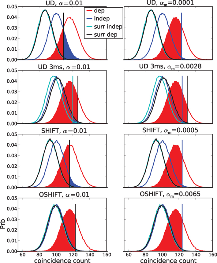
Figure 11. False positives (FP, blue areas) and false negatives (FN, red areas) for unmatched (left) and matched (right) α. The curves show coincidence count distributions of correlated (red), independent (blue) and the respective surrogate (black, cyan) data for four dithering methods (top to bottom: UD, UD 3 ms, SHIFT, OSHIFT). The probabilities at the discrete coincidence counts are connected by straight lines and the sums of neighboring probabilities are indicated by colored areas for clarity. For UD with dither width reduced to 3 ms (second row) from 20 ms the surrogate distribution for correlated data (black) is substantially shifted to the right with respect to the one for independent data (cyan). The left column shows results for a fixed significance level of α = 0.01. The coincidence count n_α (vertical bar) is the largest count with respect to the surrogate distributions for which the sum of the probabilities of increasing counts starting at this value is smaller or equal α. This defines the fraction of FP as the area under the independent distribution (blue) for counts ≥n_α and the fraction of FN as the area under the correlated distribution (red) for counts ≤n_α. For the four methods the n_α are located at different counts and for UD 3 ms also the n_α of the two surrogate distributions differ (visible cyan vertical bar). The right column shows results for FP levels of 0.01 achieved by choosing a corresponding significance level α_m (values in panel titles). The count n_FP=1% (blue vertical bar) is the largest count with respect to the independent distribution (blue curve) for which the sum of the probabilities of increasing counts starting at this value is smaller or equal FP = 1% (blue area). This α_m applied to the surrogate distribution of correlated data defines the threshold count for the fraction of FN (red area). For UD 3 ms the threshold (visible black vertical bar) is to the right of n_FP=1%. Δλ = 90 Hz, other parameters as in Figure 6.

Figure 11 illustrates the shapes of the distributions and their relationships at a particular Δλ. For the given significance level of α = 0.01 the fractions of FP and FN differ considerably between the surrogate methods. This is mainly due to the different means of the surrogate distributions. The differences between the surrogate and the independent distribution for UD and SHIFT demonstrate the fact that these surrogates lead to lower mean coincidence counts than in the independent data due to the destruction of the rate profile (cf. Figure 4). For OSHIFT the surrogate distribution well resembles the independent distribution. UD exhibits a decreased level of FN simply because compared to OSHIFT the surrogate distribution is shifted to the left. The price is an increase of FP far exceeding α because the surrogate distribution is also shifted to the left with respect to the independent distribution. For UD 3 ms the surrogate distributions are closer to the independent distribution because the rate profile is less distorted as at the larger dither width. However, at the smaller dither width the surrogate distributions for correlated and independent data are no longer identical because the method does not destroy coincidences effectively enough.

In the right column of Figure 11 we match the fraction of FP of the dithering methods at a target level of 1% by selecting the minimal coincidence count required for significance n_FP=1% as the largest coincidence count for which the total probability of the independent distribution for counts larger or equal to this value does not exceed 1%. The total probability of the surrogate distribution corresponding to n_FP=1% constitutes the matching significance level α_m of the dithering method used to generate the surrogate distribution. By definition n_FP=1% has exactly the same value for all dithering methods because it only depends on the independent distribution, not the surrogate distribution. Therefore, not only the fraction of FP but also the fraction of FN are now identical for all dithering methods. What is different is the matched significance level α_m. Clearly, this calibration procedure is only possible in our model situation because we have access to the true coincidence count distribution of independent data.

An exception to the invariance of the relationship between FP and FN with respect to the dithering methods at matched α levels is UD 3 ms. Here the surrogate method does not destroy all injected coincidences. The surrogate distribution for correlated data is shifted to the right with respect to the surrogate distribution for independent data. Therefore, the α_m determined using the independent data leads to an increased fraction of FN.

The top panel of Figure 12 shows the dependence of the fraction of FP on the magnitude of the rate step Δλ. With increasing Δλ the discreteness of the distribution of coincidence counts reduces and therefore the optimal choices of n_FP=1% better approximate the target FP fraction of 1%. A detailed discussion of the discreteness of the distribution of coincidence counts can be found in Grün (2009). All methods behave the same.

FIGURE 12

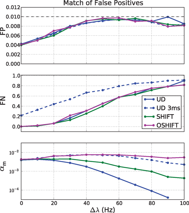
Figure 12. False negatives (FN, middle panel) at matched rates of false positives (FP, top panel) for four surrogate methods (UD, UD 3 ms, SHIFT, OSHIFT). The top panel shows the optimal approximations to the target fraction of FP = 1% given the discreteness of the coincidence count distributions at the magnitude of the rate step Δλ. The middle panel shows the corresponding fractions of FN. The bottom panel shows the significance levels α_m of the four surrogate distributions realizing the matched FP rate of 1% on a log-scaled axis. Other parameters as in Figure 11.

The fraction of FN increases with increasing Δλ (Figure 12, middle panel) because with increasing mean spike rate the fraction of surplus coincidences compared to the number of chance coincides reduces. The dependence of FN on Δλ only depends on the independent distribution and therefore is identical for all dithering methods and represents the optimal sensitivity (FN rate) for any surrogate method. An exception is UD 3 ms which does not manage to destroy the injected coincidences effectively enough. The result is a substantially reduced sensitivity. The FN converge again at large Δλ when the injected coincidences contribute little to the large number of chance coincidences.

The bottom panel of Figure 12 shows the dependence of the significance level α_m on Δλ. For OSHIFT the α_m stays close to the desired fraction of FP = 1% because the surrogate distribution well approximates the distribution of coincidence counts for independent data. Thus, using OSHIFT the experimenter can select the α of choice and obtain the expected FP level. Also UD 3 ms is well behaved in this respect. For UD at ±20 ms, however, α_m drops with increasing Δλ by at least two orders of magnitude. This indicates that n_FP=1% is located far out in the tail of the surrogate distribution. Consequently the precise value of α_m depends on the details of the time course of the original data. There is no universal mapping of a desired significance level α to α_m for UD.

In conclusion, we now understand why the performance of OSHIFT cannot be achieved by reducing the dither width of UD as studied in Figure 7. Reducing the dither width reduces the fraction of FP and increases the fraction of FN because the surrogate distribution better resembles the independent distribution. Eventually, however, the dither width is so low that a substantial fraction of injected coincidences remains intact and the fraction of FN surpasses the one for OSHIFT at a larger dither width. A good surrogate method is characterized by the congruence of three distributions: the distribution of coincidence counts of independent data, the surrogate distribution of independent data, and the surrogate distribution of correlated data.

It appears tempting to calibrate α_m on the surrogate distribution for correlated data instead of independent data to compensate for the incomplete destruction of coincidences at small dither widths. This, however, is a conceptual error in the context of our null-hypothesis because α_m then depends on the amount of synchrony originally contained in the data.