Efficient option pricing under Lévy processes, with CVA and FVA

1. Introduction

Counterparty credit risk and the cost of funding in the valuation of derivatives have become a paramount topic in the industry. Counterparty credit risk can be defined as the risk of a party to a financial contract defaulting prior to the contract's expiration and not fulfilling all of its obligations. Each party to a transaction runs the risk of a loss from the counterparty defaulting; there is also the possibility of a gain from an increase of the self-default risk which reduces the counterparty's expectation of the transaction value. The expected loss from the default of a counterparty is generally referred to as the credit valuation adjustment (CVA), whilst the expected benefit from self-default risk is referred to as debt valuation adjustment (DVA). The question of whether the gain from increasing self default risk can actually be monetized and therefore should be included in derivative valuation values remains debatable, and it is currently excluded from prudential capital calculations under CRD IV, but must be included under generally accepted accounting rule as specified under IFRS 13.

Counterparty credit risk can be mitigated by collateralization. Each party to a transaction agrees to post/receive collateral when the value of the transaction moves against / in favor of one of the party under a collateral agreement. Transactions are generally executed via central counterparties (CCP) under robust collateral agreements which require posting of both initial and variation margins, whilst regulations of over-the-counter (as proposed by the Basel Committee in September 2013) will soon also make it mandatory for both parties to post initial and variation margins. Collateral that are posted against derivative transactions generally receive risk-free returns but must be funded/borrowed at non-risk-free rates, therefore introduces an additional cost to each counterparty, and the expected value of this cost is generally referred to as funding valuation adjustment (FVA). Since collateral funding cost is a function of the collateral requirement, which in turn is a non-linear function of the value of the derivative, the pricing problem involving FVA is non-linear and hence non-trivial.

In numerous studies, these adjustments (CVA, DVA, and FVA) have been analyzed separately. Pykhtin and Zhu [3] modeled the credit exposure and priced the counterparty credit risk. Bilateral counterparty risk is analyzed in Brigo et al. [4, 5], Brigo and Morini [6], Gregory [7, 8]. In a series of papers, Alex Lipton with co-authors developed several efficient methods for pricing bilateral counterparty risk for CDS. In 2-3 factor structural models driven by the Brownian motion, quasi-analytical formulas are developed [9, 10]; in jump-diffusion models [11], an efficient numerical algorithm is designed. For further details and references, see [9–13].

An initial analysis of collateralization and funding risk in is due to Piterbarg [1]. Debates for funding valuation adjustment continue in Burgard and Kjaer [2] Hull and White [14], Castagna [15]. Further generalizations appear in Burgard and Kjaer [16, 17], Lu and Juan [18], Wu [19] which resort to a PDE approach, while Brigo et al. [20, 21], Pallavicini [22], Brigo and Pallavicini [23], Pallavicini et al. [24], Brigo and Pallavicini [25], Brigo [26] use the no-arbitrage approach. The models in these papers are of the reduced type.

In the paper, we consider a generalization of Piterbarg's [1] pricing equation. The equation is non-linear due to the presence of the term that accounts for the funding risk; the necessity of taking into account the collateral requirement and counterparty risk leads to additional complications. A simple natural remark (already made in Brigo et al. [20] and Kenyon and Stamm [27]) is that in a non-linear problem, it is impossible to separate effects of the funding value adjustment (FVA) and CVA; we produce an example which shows that the difference between the exact result in the non-linear problem, which takes both effects into account simultaneously, and the sum of two effects calculated separately can differ by a wide margin.

A rigorous study of such a complicated situation requires an explicit specification of objective functions of agents involved (the trader and the treasury/XVA desk), and the result of such a study will strongly depend on these objective functions and the bargaining power of the agents involved. We leave this study for the future. In the present paper, we make the following simplifying assumption which is close but not identical to the remark made by Piterbarg [1]. Namely, we assume that, outside the bank where FVA and CVA need to be taken into account, there exists a large, liquid, and, essentially, frictionless market for the underlying security so that, if one forgets about the tiny segment of the market related to the bank in question (or, at least, to the trader inside a large bank), one can assume that all streams of payoffs can be priced under some equivalent martingale measure. If the trader is not the London Whale, this assumption is relatively reasonable. An additional justification for this assumption is that, by the very nature of the conditions in this tiny segment (once again, we have to assume away the possibility that the trader turns out to be the next London Whale), the payoff streams involve sizable frictions, therefore, should some formal arbitrage opportunities arise, they cannot be realized due to the presence of additional costs such as different rates for opposite sides of transactions.

Under the above assumption, we therefore use an “exterior” equivalent martingale measure (EMM) to price all flows inside the tiny submarket that involves the trader and treasury/XVA desk. However, we explicitly take into account the rules of the asset pricing inside this tiny market that are specified by the regulatory requirements. We leave for the future an extremely important question whether these requirements are rational or not.

The paper organized as follows. The model is described in detail In Section 2, we formulate the model in detail, and formulate non-linear boundary problems for different types of options. Section 3 describes the Carr's randomization algorithm for the problem and its realization. The detailed numerical scheme are derived in Section 4, and explicit algorithms are formulated in Section 5. Numerical examples are given in Section 6, and Section 7 concludes. Technical details are relegated to Appendices.

2. The Model

2.1. A generalization of Piterbarg's pricing equation

Assume that, apart from the security that we model, the market is void of frictions and arbitrage free. Then, under additional technical regularity conditions, there exists an equivalent measure ℚ such that the price of any security traded in the market is the expected value of discounted instantaneous payoffs and payoff streams that the security gives the right to, under ℚ. Assume also that, under ℚ, the discounted prices of all securities are functions of a strong Markov process $\tilde{X}$ with the infinitesimal generator ${ℒ}$, and of time. Then, in the region of the time-state space where the security remains alive its price obeys the generalized Black-Scholes equation

$\begin{array}{rc}({\partial }_t+{ℒ})V(t,\tilde{x})+g(t,\tilde{x})=0,& (2.1)\end{array}$

where $g(t,{\tilde{X}}_t)$ is the stream of payoffs during the security's life-time, subject to appropriate terminal and boundary conditions, which specify $V(t,{\tilde{X}}_t)$ at expiry.

In short rate models, it is natural to regard X as the process with killing, and explicitly write the infinitesimal generator in the form ${ℒ}$ = L − r, where L is the infinitesimal generator of the corresponding Markov process without killing, and r is the multiplication-by-$r=r(t,\tilde{x})$ operator; then Equation (2.1) becomes

$\begin{array}{rc}({\partial }_t+L-r(t,\tilde{x}))V(t,\tilde{x})+g(t,\tilde{x})=0.& (2.2)\end{array}$

The constructions below can be easily generalized to the case of the stochastic interest rate; the rate can be time-dependent. However, in the present paper, we assume that the riskless rate r is constant; moreover, the stochastic factor is assumed to be a Lévy process X on ℝ, and, apart from the riskless bond, there is only one underlying stock or index modeled as $S_t=e^{X_t}$. Then Equation (2.2) simplifies further:

$\begin{array}{rc}({\partial }_t+L-r)V(t,x)+g(t,x)=0.& (2.3)\end{array}$

If the external market is the Black-Scholes market, then Equation (2.3) is

$\begin{array}{rc}\left({\partial }_t+\frac{{\sigma }^2}{2}{\partial }_x^2+(r-{\sigma }^2∕2){\partial }_x-r\right)V(t,x)+g(t,x)=0.& (2.4)\end{array}$

In the model, which takes into account all the payments related to required collateral posting and funding, the stream of the total payoffs during the life-time of the contingent claim becomes rather involved. What is very important, and what makes the whole idea of the no-arbitrage pricing in the presence of FVA incorrect, strictly speaking, is the non-linearity of the pricing equation. Indeed, as it is shown below, the payoff stream g(t, x) depends on the value function V itself, and in a non-linear manner. However, the no-arbitrage pricing is linear. Therefore, the Equation (2.3) with g(V; t, x) below makes sense only as an approximation, if we presume that the effect of the contingent claim under consideration on the whole market is vanishingly small and can be ignored.

Before we go into the description of the stream g(V; t, x), we introduce the notation that we use throughout the paper. Let A be the bank and B be its counterparty. Assume A and B agree to the ISDA agreement to set out standard terms that apply to all deals between them. The credit support annex (CSA) to the ISDA master agreement defines the rules under which the collateral is posted between A and B. The stream comes from several sources of cashflow:

(1) The stream that accounts for the cost of collateral posting/receiving. The stream is (r − r_C)C, where r_C is the collateral rate (for example the US effective FED rate).

(2) The stream that accounts for the cost of unsecured funding. The stream for unsecured funding is (r − r_F)(V − C), where r_F is the unsecured funding rate.

(3) The on-default cashflow. The stream is

$\begin{array}{r}(1-R_A)\lambda (V^{-}-C)-(1-R_B)\lambda (V^{+}-C),\end{array}$

where V⁺ = max{V, 0}, V⁻ = min{V, 0}, R_i is the recovery rate respectively for i = A, B, and λ is the first-to-default intensity.

The collateral depends on V, and it is given by

$\begin{array}{cc}C=C(V)=\{\begin{array}{ll}{(V-H_B)}^{+},\hfill & \text{if }V>0,\hfill \\ -{(-V-H_A)}^{+},\hfill & \text{if }V<0,\hfill \end{array}& (2.5)\end{array}$

where H_A, H_B are the collateral thresholds for A and B, respectively, and C is the collateral of A. C is taken to be positive if the counterparty (B) posts collateral to A, and is negative if the counterparty receives collateral from A. We assume that R_i, λ, H_i are constants, hence, the stream of payoffs can be considered as a function of one argument V; naturally, the composite function g(V) is a function of t, x.

Adding up these streams, we obtain the following equality

$\begin{array}{c}g(V)=(r-r_C)C+(r-r_F)(V-C)\hfill \\ +(1-R_A)\lambda (V^{-}-C)-(1-R_B)\lambda (V^{+}-C).(2.6)\hfill \end{array}$

The two extremes are uncollateralized and fully collateralized cases considered in Piterbarg [1], Antonov et al. [28]. In the former case, C = 0, hence the stream is

$g(V)=(r-r_F)V+(1-R_A)\lambda V^{-}-(1-R_B)\lambda V^{+}.$

In the latter case, C = V, hence the stream is g(V) = (r − r_C)C = (r − r_C)V. See Appendix B.1 for details.

Remark 2.1. In the paper, we consider option pricing, and V is either non-negative (the long side of the contract) or non-positive (short side). For general financial instruments, V can assume positive and negative value (e.g., swaps, forwards, CDSs).

2.2. Detalization of the Model: Processes

The underlying stock or index is modeled as $S_t=e^{X_t}$, where X is a Lévy process on ℝ (for applications of Lévy processes in risk predictions in high frequency trading, see [29]), with the infinitesimal generator L and characteristic exponent ψ. Making the change of variables τ = T − t, we rewrite Equation (2.3) as

$\begin{array}{rc}({\partial }_{\tau }-L+r)V=g(V),\tau >0.& (2.7)\end{array}$

Recall that the characteristic exponent of a Lévy process X = {X_t}_{t ≥ 0} is a continuous function ψ:ℝ → ℂ satisfying ψ(0) = 0 and

$\begin{array}{rc}𝔼\left[e^{i\xi X_t}\right]=e^{-t\psi (\xi )}\forall \xi \in ℝ,t\ge 0.& (2.8)\end{array}$

From now on we will assume that there exist λ₋ < −1 < 0 < λ₊ such that the underlying Lévy process X is of the exponential type (λ₋, λ₊). Roughly speaking, this means that the characteristic exponent ψ(ξ) admits analytic continuation into the open strip Im ξ ∈ (λ₋, λ₊). Moreover, ψ(ξ) grows at most polynomially as Re ξ → ±∞ within every closed strip Im ξ ∈ [ω₋, ω₊] ⊂ (λ₋, λ₊). A precise formulation (in terms of the Lévy density of X) is given in Boyarchenko and Levendorskiĭ [30, Definition 3.2]. The details are not important to us: for the applications we have in mind, it will suffice to know that the examples below satisfy the definition.

1. A Brownian motion (used in the classical Black-Scholes model [31]) is a Lévy process of exponential type (−∞, ∞). Its characteristic exponent is given by $\frac{{\sigma }^2}{2}{\xi }^2-i\mu \xi$, where σ > 0 is the volatility and μ ∈ ℝ is the drift of the process.

2. In Merton's model [32], the underlying log-price process is a Lévy process with characteristic exponent $\psi (\xi )=\frac{{\sigma }^2}{2}{\xi }^2-i\mu \xi +\lambda ·\left(1-e^{im\xi -\frac{s^2}{2}{\xi }^2}\right)$, where σ, s, λ > 0 and μ, m ∈ ℝ. A process of this kind also has exponential type (−∞, ∞).

3. A hyper-exponential jump-diffusion process introduced in Lipton [33], Levendorskiĭ [34] and studied in detail in Levendorskiĭ [34, 35] has characteristic exponent

$\begin{array}{rc}\psi (\xi )=\frac{{\sigma }^2}{2}{\xi }^2-i\mu \xi +{\lambda }^{+}·{\displaystyle \sum _{j=1}^{n^{+}}}\frac{i{p}_j^{+}\xi }{i\xi -{\alpha }_j^{+}}+{\lambda }^{-}·{\displaystyle \sum _{k=1}^{n^{-}}}\frac{i{p}_k^{-}\xi }{i\xi +{\alpha }_k^{-}},& (2.9)\end{array}$

where n^± are positive integers and ${\alpha }_j^{\pm },{\lambda }^{\pm },p_j^{\pm }>0$ satisfy $\sum _{j=1}^{n^{\pm }}{p}_j^{\pm }=1$. The double-exponential jump-diffusion model (DEJD) model [33, 36, 37], which was discovered earlier, can be obtained as a special case of hyper-exponential jump-diffusion models by taking n⁺ = n⁻ = 1. A Lévy process with characteristic exponent Equation (2.9) is of exponential type $(\max \{-{\alpha }_k^{-}\},\min \{{\alpha }_j^{+}\})$.

4. Lévy processes of the extended Koponen family (generalizing the class of processes introduced by Koponen [38]) were constructed by Boyarchenko and Levendorskiĭ [39]. A somewhat narrower class of processes was labeled later KoBoL processes or KoBoL model [30]. A subclass of KoBoL has become popular under the name CGMY model [40]. The characteristic exponent of a KoBoL process of order ν ∈ (0, 2), ν ≠ 1, has the form¹

$\begin{array}{l}\psi (\xi )=-i\mu \xi +c·\Gamma (-\nu )·[{(-{\lambda }_{-})}^{\nu }-{(-{\lambda }_{-}-i\xi )}^{\nu }+{\lambda }_{+}^{\nu }\\ -{({\lambda }_{+}+i\xi )}^{\nu }],& (2.10)\end{array}$

where λ₋ < 0 < λ₊ are called the steepness parameters of the process, c > 0 is its intensity, and μ ∈ ℝ. A KoBoL process with parameters as above has exponential type (λ₋, λ₊), so there is no conflict of notation.

5. Variance Gamma (V.G.) processes were first used in empirical studies of financial markets by Madan and collaborators [41–43]. The characteristic exponent of a V.G. process has the form²:

$\begin{array}{l}\psi (\xi )=-i\mu \xi +c·[\ln (-{\lambda }_{-}-i\xi )-\ln (-{\lambda }_{-})+\ln ({\lambda }_{+}+i\xi )\\ -\ln ({\lambda }_{+})],& (2.11)\end{array}$

where λ₋ < 0 < λ₊, c > 0 and μ ∈ ℝ. A V.G. process with these parameters is also a Lévy process of exponential type (λ₋, λ₊).

6. Normal Inverse Gaussian (NIG) processes were introduced to finance by Barndorff-Nielsen [44]. The characteristic exponent of a NIG process is of the form

$\begin{array}{rc}\psi (\xi )=-i\mu \xi +\delta ·\left[{\left({\alpha }^2-{(\beta +i\xi )}^2\right)}^{1∕2}-{({\alpha }^2-{\beta }^2)}^{1∕2}\right],& (2.12)\end{array}$

where α > |β| > 0, δ > 0 and μ ∈ ℝ. A NIG process with these parameters has exponential type (β − α, β + α).

Other examples of Lévy processes of exponential type can be found in Boyarchenko and Levendorskiĭ [30, Ch. 3] and Kuznetsov [45], Kuznetsov et al. [46].

2.3. Boundary Problem for Different Options with CVA and FVA

2.3.1. European Option with CVA and FVA

Let V_Eur.(t, X_t) be the price of an European option with maturity T, strike K and a bounded payoff function G(x). Then V_Eur.(t, X_t) is a unique bounded solution of the boundary problem

$\begin{array}{rcll}({\partial }_{\tau }-L+r)V(\tau ,x)& =& g(V(\tau ,x)),\tau >0,& (2.13)\end{array}$

$\begin{array}{rcll}V(0,x)\hfill & =\hfill & G(x).\hfill & (2.14)\hfill \end{array}$

If G is unbounded, the call option being the main example, then an appropriate condition of the characteristic exponent must be imposed to ensure the finiteness of the option price, and the solution of the boundary problem Equation (2.13) sought for in the class of functions subject to the corresponding restriction on the rate of growth at infinity. See [30] for details.

2.3.2. Down-and-out Barrier Put Option with CVA and FVA

Let V_d.o.put(t, X_t) be the price of the down-and-out put option with maturity T, strike K and barrier H < K. Let h = ln H. Then V_d.o.put(t, X_t) is a unique bounded solution of the boundary problem

$\begin{array}{rcll}({\partial }_{\tau }-L+r)V(\tau ,x)\hfill & =\hfill & g(V(\tau ,x)),x>h,\tau >0,\hfill & (2.15)\hfill \end{array}$

$\begin{array}{rcll}V(0,x)\hfill & =\hfill & {(K-e^x)}_{+}{𝟙}_{(h,+\infty )}(x),\hfill & (2.16)\hfill \end{array}$

$\begin{array}{rcll}V(\tau ,x)\hfill & =\hfill & 0,x\le h.\hfill & (2.17)\hfill \end{array}$

2.3.3. Down-and-in First Touch Digital Option with CVA and FVA

Let V_f.t.d.(t, X_t) be the price of the down-and-in first touch digital option with maturity T and barrier H. Let h = ln H. Then V_f.t.d.(t, X_t) is a unique bounded solution of the boundary problem

$\begin{array}{rcll}({\partial }_{\tau }-L+r)V(\tau ,x)\hfill & =\hfill & g(V(\tau ,x)),x>h,\tau >0,\hfill & (2.18)\hfill \end{array}$

$\begin{array}{rcll}V(0,x)\hfill & =\hfill & {𝟙}_{(-\infty ,h]}(x),\hfill & (2.19)\hfill \end{array}$

$\begin{array}{rcll}V(\tau ,x)\hfill & =\hfill & 1,x\le h,\tau \ge 0.\hfill & (2.20)\hfill \end{array}$

In the next section, we will use the Carr's randomization and backward induction to solve the boundary problems for European options and barrier options, with CVA and FVA.

3. Wiener-Hopf Factorization and Carr's Randomization

3.1. Three Forms of WHF

Define the supremum process $\overline{X}$ and the infimum process X of X by

$\begin{array}{rc}{\overline{X}}_t={\displaystyle \underset{0\le s\le t}{sup}}{X}_s,{{\displaystyle \underset{\_}{X}}}_t={\displaystyle \underset{0\le s\le t}{inf}}{X}_s.& (3.1)\end{array}$

Given any q > 0, we let T_q ~ Exp q denote an exponentially distributed random variable with mean q⁻¹. The form of the Wiener-Hopf factorization (WHF) formula that is commonly used in probability theory is as follows:

$\begin{array}{rc}𝔼\left[e^{i\xi X_{T_q}}\right]=𝔼\left[e^{i\xi {\overline{X}}_{T_q}}\right]·𝔼\left[e^{i\xi {{\displaystyle \underset{\_}{X}}}_{T_q}}\right]\forall \xi \in ℝ.& (3.2)\end{array}$

Introducing the Wiener-Hopf factors ${\varphi }_q^{+}(\xi )=𝔼\left[e^{i\xi {\overline{X}}_{T_q}}\right]$, ${\varphi }_q^{-}(\xi )=𝔼\left[e^{i\xi {\underset{\_}{X}}_{T_q}}\right]$, we can rewrite Equation (3.2) as a special case of the analytical form of the Wiener-Hopf factorization formula:

$\begin{array}{rc}\frac{q}{q+\psi (\xi )}={\varphi }_q^{+}(\xi ){\varphi }_q^{-}(\xi ).& (3.3)\end{array}$

Since the trajectories of the supremum process $\overline{X}$ are nondecreasing, ${\varphi }_q^{+}(\xi )$ admits analytic continuation into the upper half-plane. Similarly, ${\varphi }_q^{-}(\xi )$ admits analytic continuation into the lower half-plane. Thus, Equation (3.3) is a special case of the Wiener-Hopf factorization of a function defined on the real axis, which historically was the first form of the WHF formula.

Define operators ${{ℰ}}_q^{+}$ and ${{ℰ}}_q^{-}$ acting on nonnegative measurable (or an arbitrary bounded measurable) functions f on ℝ as follows:

$\begin{array}{rc}({{ℰ}}_q^{+}f)(x)={𝔼}^x\left[f({\overline{X}}_{T_q})\right],({{ℰ}}_q^{-}f)(x)={𝔼}^x\left[f({{\displaystyle \underset{\_}{X}}}_{T_q})\right].& (3.4)\end{array}$

We also define the EPV operator ${{ℰ}}_q$ of the process X itself by

$\begin{array}{rc}({{ℰ}}_{q}f)(x)={𝔼}^x\left[f(X_{T_q})\right].& (3.5)\end{array}$

The operator form of the WHF formula is

$\begin{array}{rc}{{ℰ}}_q={{ℰ}}_q^{+}{{ℰ}}_q^{-}={{ℰ}}_q^{-}{{ℰ}}_q^{+}& (3.6)\end{array}$

(see [30, 47, 48]).

3.2. Carr's Randomization and Backward Induction with CVA and FVA

Carr's randomization [49] is an approximation procedure that replaces the problem of pricing a finite-lived option with a sequence of option pricing problems for perpetual options. These problems can be solved in closed form that is amenable to very fast numerical calculations using the operator form of the Wiener-Hopf factorization method developed in a series of works by Boyarchenko and Levendorskiĭ [30, 48, 50, 51]. The maturity period of the claim is divided into N subintervals, using points 0 = t₀ < t₁ < … < t_N = T, and each sub-period [t_s, t_{s + 1}] is replaced with an exponentially distributed random maturity period with mean Δ_s = t_{s + 1} − t_s. Moreover, these N random maturity sub-periods are assumed to be independent of each other and of the process X. (In Carr [49], it is assumed that Δ_s = T∕N for all s, but, in principle, we do not have to impose this requirement).

Denote by V_s(x) the Carr's randomization approximation to V(t_N−s, x). Then, by definition, V₀(x) = G(x), the terminal payoff function.

3.2.1. Carr's Randomization for Down-and-Out Barrier Options with CVA and FVA

For all 0 ≤ s ≤ N − 1, the function V_{s + 1}(x) is the value function of a down-and-out barrier contingent claim with barrier H = e^h, terminal payoff function V_s(x), and exponentially distributed maturity date with mean Δ_s and a nonlinear stream g(V_s(x)). In particular, V_s(x) = 0, x ≤ h, s = 0, 1, …, N.

Then, we discretize the time derivative in equation Equation (2.15) by a finite difference and rewrite Equation (2.15) in the implicit-explicit form: for s = 0, 1, …, N − 1,

$\begin{array}{rc}\frac{V_{s+1}(x)-V_s(x)}{{\Delta }_s}+(r-L)V_{s+1}(x)=g(V_s(x)),x>h.& (3.7)\end{array}$

We define $q_s=r+{\Delta }_s^{-1}$, and rewrite Equation (3.7) as

$\begin{array}{rc}(q_s-L)V_{s+1}(x)=f_s(x),x>h,& (3.8)\end{array}$

where $f_s:={\Delta }_s^{-1}{V}_s+g(V_s)$. By Lemma 2.1 in [48], we have, for s = 0, 1, …, N − 1,

$\begin{array}{rc}{V}_{s+1}=q_s^{-1}{{ℰ}}_{q_s}^{-}{𝟙}_{[h,+\infty )}{{ℰ}}_{q_s}^{+}{f}_s.& (3.9)\end{array}$

The function V_N(x) obtained at the last step of this algorithm is the Carr's randomization approximation to Equation (2.15). It is possible to prove that, as the mesh $\underset{s}{max}{\Delta }_s$ of the partition of the maturity period of the claim approaches 0, V_N(x) converges to V(x).

3.2.2. Carr's Randomization for European options with CVA and FVA

In this case, Equation (3.8) holds on the whole line. Using the well-known equality ${{ℰ}}_q=q{(q-L)}^{-1}$ (see, e.g., [30, 47])), we obtain, for s = 0, 1, …, N − 1,

$\begin{array}{rc}{V}_{s+1}(x)=q_s^{-1}({{ℰ}}_{q_s}{f}_s)(x),x\in ℝ.& (3.10)\end{array}$

3.2.3. Carr's Randomization for First-Touch Digital Option

For all s and x ≤ h, V_{s + 1}(x) = 1, and V₀(x) = 0, x > h. By Lemma 2.3 in Boyarchenko and Levendorskiĭ [48], we have, for s = 0, 1, …, N − 1,

$\begin{array}{rc}{V}_{s+1}={{ℰ}}_{q_s}^{-}\left({𝟙}_{(-\infty ,h]}+q_s^{-1}{𝟙}_{[h,+\infty )}{{ℰ}}_{q_s}^{+}{f}_s\right).& (3.11)\end{array}$

4. Numerical Realization of the Action of EPV Operators

4.1. EPV Operators Via Convolution

The formulas are as follows:

$\begin{array}{rcl}({{ℰ}}_{q}f)(x)& =& {\displaystyle {\int }_{-\infty }^{\infty }}f(x+y)g_q(y)dy,\\ ({{ℰ}}_q^{\pm }f)(x)& =& {\displaystyle {\int }_{-\infty }^{\infty }}f(x+y)g_q^{\pm }(y)dy,& (4.1)\end{array}$

with the convolution kernels being given by

$\begin{array}{rcl}{g}_q(y)& =& \frac{1}{2\pi }{\displaystyle {\int }_{-\infty }^{\infty }}\frac{q{e}^{-iy\xi }d\xi }{q+\psi (\xi )},\\ g_q^{\pm }(y)& =& \frac{1}{2\pi }{\displaystyle {\int }_{-\infty }^{\infty }}{\varphi }_q^{\pm }(\xi )e^{-iy\xi }d\xi ,& (4.2)\end{array}$

where ψ(ξ) is the characteristic exponent of X (cf. Section 2.2) and ${\varphi }_q^{\pm }(\xi )$ are the Wiener-Hopf factors of q(q + ψ(ξ))⁻¹, defined by ${{ℰ}}_q^{\pm }(e^{i\xi x})={\varphi }_q^{\pm }(\xi )e^{i\xi x}$. In this subsection and the next three subsections and Appendix A, we reproduce the detailed prescription from Boyarchenko and Levendorskiĭ [48, 51] for calculation of ${\varphi }_q^{\pm }$, and refer the reader to Boyarchenko and Levendorskiĭ [48, 51], Sato [52] for background on the Wiener-Hopf factorization. Note that if X is a process of finite variation with positive (resp., negative) drift, then the measure g⁺(y)dy has an atom at 0 (resp., the measure g⁻(y)dy has an atom at 0). In such cases, the corresponding equality in Equation (4.2) is valid for y ≠ 0 only. For the numerical calculations below this subtlety does not really matter because we will use Equation (4.2) for calculations outside the origin only.

4.2. Integral Formulas for the WH Factors

We now suppose that there exist λ₋ < 0 < λ₊ such that the Lévy process X is of exponential type (λ₋, λ₊). (cf. Section 2.2). Under a certain regularity assumption on the characteristic exponent ψ(ξ) of X (see, e.g., [30, Theorem 3.2]), Boyarchenko and Levendorskiĭ obtained integral formulas for the Wiener-Hopf factors ${\varphi }_q^{\pm }(\xi )$. This assumption holds in all model examples of Lévy processes of exponential type, including those listed in Section 2.2, so we prefer not to state it to save space. The formulas [30, Equations (3.58), (3.60)] are as follows:

$\begin{array}{rc}{\varphi }_q^{\pm }(\xi )=exp\left[\pm \frac{1}{2\pi i}{\displaystyle {\int }_{Im\eta ={\omega }_{\mp }}}\frac{\xi ·ln(1+q^{-1}\psi (\eta ))}{\eta (\xi -\eta )}d\eta \right].& (4.3)\end{array}$

Here, ω_± are real numbers such that λ₋ < ω₋ < 0 < ω₊ < λ₊, and such that there exists δ > 0 with Re(q + ψ(η)) ≥ δ whenever Im η ∈ [ω₋, ω₊].

4.3. Enhanced Realization of Convolution Operators

Let us consider one of the formulas Equation (4.1), or the definition of the Fourier transform. With the standard approach to the numerical realization of these formulas, one truncates the improper integral on the right hand side replacing it with an integral over a bounded interval, and uses a suitable quadrature rule to approximate the latter integral with a finite sum. However, it is demonstrated in Boyarchenko and Levendorskiĭ [48, 51] that sometimes this approach leads to very large computational errors, and the following alternative has been suggested: instead of discretizing the integral on the right hand side of Equation (4.1), one should first approximate the function f(x) with a piecewise linear function, and then evaluate the resulting integral involving this piecewise linear approximation explicitly (in a suitable sense).

Given functions f(x), g(x) defined on ℝ, we would like to approximately calculate

$\begin{array}{rc}F(x)={\displaystyle {\int }_{-\infty }^{\infty }}f(x+y)g(y)dy.& (4.4)\end{array}$

In order to discretize the problem, we assume given a uniformly spaced grid of points $\overrightarrow{x}={(x_j)}_{j=1}^M$, where x_j = x₁+(j − 1)Δ ∈ ℝ, and Δ > 0 is fixed. Let us write f_j = f(x_j) for all j. Following the strategy we just described, we approximate f(x) with a linear function on each of the intervals [x_j, x_j+1]:

$\begin{array}{rc}f(x)\approx f_j+{\Delta }^{-1}·(f_{j+1}-f_j)·(x-x_j),x_j\le x\le x_{j+1}.& (4.5)\end{array}$

Of course, Equation (4.5) is an exact equality for x = x_j and for x = x_{j + 1}; inside the interval (x_j, x_{j + 1}), the error of this approximation is controlled by the size of the second derivative f″(x) (assuming that the latter exists).

The next result is obtained by a straightforward computation.

Proposition 4.1. Let us approximate f(x) by a piecewise linear function on the interval [x₁, x_M] using Equation (4.5), and let us approximate f(x) by 0 outside of [x₁, x_M]. This leads to the following approximation of the values of the function F(x):

$\begin{array}{rc}F(x_k)\approx -c_k^1·f_1-(c_{k-M}^0-c_{k-M}^1)·f_M+{\displaystyle \sum _{j=1}^M}{c}_{k-j}^{\Delta }·f_j,& (4.6)\end{array}$

where f_j = f(x_j), and the coefficients $c_{\ell }^0$, $c_{\ell }^1$, $c_{\ell }^{\Delta }$ (for ℓ ∈ ℤ) are defined by

$c_{\ell }^0={\displaystyle {\int }_0^{\Delta }}g(y-\ell \Delta )dy,c_{\ell }^1={\Delta }^{-1}{\displaystyle {\int }_0^{\Delta }}y·g(y-\ell \Delta )dy,$

$\text{ and}{c}_{\ell }^{\Delta }=c_{\ell }^0-c_{\ell }^1+c_{\ell +1}^1.$

Remark 4.2. The values of the sum on the right hand side of Equation (4.6) can be computed efficiently for all 1 ≤ k ≤ M using the algorithm presented in Section A.1.3.

4.4. Enhanced Realization of the EPV Operators

In this subsection we recall the formulas for the enhanced convolution realization of the operators ${{ℰ}}_q$ and ${{ℰ}}_q^{\pm }$ that were obtained in [51, Section 4]. We keep the notation and assumptions of Section 4.1.

4.4.1. Numerical Realization of ${{ℰ}}_q$

We quote [51, Prop. 4.1]:

Proposition 4.3. In the situation of Proposition 1, let g(y) = g_q(y) be given by Equation (4.2). Then the coefficients $c_{\ell }^0$, $c_{\ell }^1$ and $c_{\ell }^{\Delta }$ can be found from the following formulas:

$c_{\ell }^0=\frac{\Delta }{2\pi }{\displaystyle {\int }_{-\infty }^{\infty }}{e}^{i\ell \Delta \xi }·\frac{q{c}_0(\xi )d\xi }{q+\psi (\xi )},$

$c_{\ell }^1=\frac{\Delta }{2\pi }{\displaystyle {\int }_{-\infty }^{\infty }}{e}^{i\ell \Delta \xi }·\frac{q{c}_1(\xi )d\xi }{q+\psi (\xi )},$

$c_{\ell }^{\Delta }=\frac{\Delta }{2\pi }{\displaystyle {\int }_{-\infty }^{\infty }}{e}^{i\ell \Delta \xi }·\frac{q{c}_{\Delta }(\xi )d\xi }{q+\psi (\xi )},$

where

$c_0(\xi )=\frac{1-e^{-i\xi \Delta }}{i\xi \Delta },c_1(\xi )=\frac{1-e^{-i\xi \Delta }-i\xi \Delta e^{-i\xi \Delta }}{{(i\xi \Delta )}^2},$

and

$c_{\Delta }(\xi )=\frac{e^{i\xi \Delta }+e^{-i\xi \Delta }-2}{{(i\xi \Delta )}^2}.$

Remark 4.4. The apparent singularities of the functions c₀(ξ), c₁(ξ) and c_Δ(ξ) at ξ = 0 are, of course, removable, as one can easily verify using the power series expansion of the exponential function.

Remark 4.5. Let us comment on the question of calculating the coefficients $c_{\ell }^0,c_{\ell }^1,c_{\ell }^{\Delta }$ appearing in Proposition 4.3. We restrict attention to $c_{\ell }^{\Delta }$ (the other ones can be treated similarly). Analyzing formula Equation (4.6) of Proposition 1, we see that, in practice, we need to compute ${(c_{\ell }^{\Delta })}_{\ell =1-M}^{M-1}$, which can be interpreted as the array of values of the inverse Fourier transform of the function

$g_q^{\Delta }(\xi )=\frac{q\Delta ·c_{\Delta }(\xi )}{q+\psi (\xi )}=q\Delta ·\frac{e^{i\xi \Delta }+e^{-i\xi \Delta }-2}{(q+\psi (\xi ))·{(i\xi \Delta )}^2}$

on the grid ${(\ell \Delta )}_{\ell =1-M}^{M-1}$. Hence this array can be calculated approximately using the inverse fast Fourier transform.

4.4.2. Numerical Realization of ${{ℰ}}_q^{+}$

The enhanced convolution realization of ${{ℰ}}_q^{+}$ is slightly easier because the kernel of ${{ℰ}}_q^{+}$ is supported on [0, +∞) (this is immediate from the interpretation of ${{ℰ}}_q^{+}$ as a normalized EPV operator for the supremum process of X). Thus, with the notation of Proposition 1, we have $c_{\ell }^0=0=c_{\ell }^1$ for ℓ > 0, which leads to the following approximation:

$({{ℰ}}_q^{+}f)(x_k)\approx -(c_{+,k-M}^0-c_{+,k-M}^1)·f_M+{\displaystyle \sum _{j=k}^M}{c}_{k-j}^{+}·f_j(1\le k\le M),$

where f_j = f(x_j) for 1 ≤ j ≤ M, and

$c_{+,\ell }^0-c_{+,\ell }^1=\frac{\Delta }{2\pi }{\displaystyle {\int }_{-\infty }^{\infty }}{e}^{i\ell \Delta \xi }·{\varphi }_q^{+}(\xi )·\frac{e^{-i\xi \Delta }+i\xi \Delta -1}{{(i\xi \Delta )}^2}d\xi$

for 1 − M ≤ ℓ ≤ 0, and

$\begin{array}{l}{c}_{\ell }^{+}=c_{+,\ell }^0-c_{+,\ell }^1+c_{+,\ell +1}^1=\frac{\Delta }{2\pi }{\displaystyle {\int }_{-\infty }^{\infty }}{e}^{i\ell \Delta \xi }·{\varphi }_q^{+}(\xi )\\ ·\frac{e^{i\xi \Delta }+e^{-i\xi \Delta }-2}{{(i\xi \Delta )}^2}d\xi \end{array}$

for 1 − M ≤ ℓ ≤ 0.

Remark 4.6. The obvious analogue of Remark 4.5 is valid here as well, the only difference being that in order to calculate the convolution coefficients $c_{\ell }^{+}$ and $c_{+,\ell }^0-c_{+,\ell }^1$, we must first calculate the array of values of ${\varphi }_q^{+}(\xi )$ on a suitable grid in the ξ-space using the algorithm of Section A.1.1 (where “suitable” means “suitable for the application of the refined iFFT technique of Boyarchenko and Levendorskiĭ [48, 51]).

4.4.3. Numerical Realization of ${{ℰ}}_q^{-}$

The situation is similar to that of Section 4.4.2, except that if we view ${{ℰ}}_q^{-}$ as a convolution operator, then its kernel is supported on (−∞, 0]. Thus, with the notation of Proposition 1, we have $c_{\ell }^0=0=c_{\ell }^1$ for ℓ ≤ 0, which leads to the following approximation:

$({{ℰ}}_q^{-}f)(x_k)\approx -c_{-,k}^1·f_1+{\displaystyle \sum _{j=1}^k}{c}_{k-j}^{-}·f_j(1\le k\le M),$

where f_j = f(x_j) and

$c_{-,\ell }^1=\frac{\Delta }{2\pi }{\displaystyle {\int }_{-\infty }^{\infty }}{e}^{i(\ell -1)\Delta \xi }·{\varphi }_q^{-}(\xi )·\frac{e^{i\xi \Delta }-i\xi \Delta -1}{{(i\xi \Delta )}^2}d\xi$

for 1 ≤ ℓ ≤ M, and

$\begin{array}{l}{c}_{\ell }^{-}=c_{-,\ell }^0-c_{-,\ell }^1+c_{-,\ell +1}^1=\frac{\Delta }{2\pi }{\displaystyle {\int }_{-\infty }^{\infty }}{e}^{i\ell \Delta \xi }·{\varphi }_q^{-}(\xi )\\ ·\frac{e^{i\xi \Delta }+e^{-i\xi \Delta }-2}{{(i\xi \Delta )}^2}d\xi \end{array}$

for 0 ≤ ℓ ≤ M − 1.

4.5. Correction for the Approximation

In previous section, we explain the backward induction scheme for CVA and FVA using the EPV operators and their realizations. As one may expect the non-linear stream would may lead to sizeable errors due to a large number of steps in the backward induction scheme. We introduce a correction term to overcome this problem. The suggested method is relatively straightforward.

4.5.1. Presence of Kinks

We use piecewise linear function to approximate the function f_s(x) = q_sV_s(x) − g(V_s(x)) in the convolution realization. In general, the stream g has three kinks at V_s = {−H_A, 0, H_B}. The piecewise linear approximation may give an inaccurate approximation to g at these points in the backward induction scheme. Hence a correction should be added in each step of the backward induction. Since we consider a long position on a European put option whose value function is positive, there is only a single kink at V_s = H_B.

Denote V_s,i = V_s(x_i), and let x′ be the kink of V_s. We the smallest V_i such that V_i ≥ H_B, that is V_i = min{V : V ≥ H_B}, and if is not large, then we use the linear interpolation to locate the kink x′:

$x^{\prime }=x_i+\frac{H_B-V_{s,i}}{V_{s,i+1}-V_{s,i}}\Delta .$

Since the price of the European put decays fast as x → +∞, there is no significant gain in taking the kink into account if x′ >> 1. Thus, we find the kink (approximately) only if V_s,i+1 − V_s,i is not negligibly small.

4.5.2. Calculating the Correction

The correction can be calculated using the standard Fourier transform technique. In Figure 1, the solid line is the approximation given by piecewise linear function and the dashed line is the exact g. The correction term is the price of the European option with the payoff G(x) that is the difference between the dashed line payoff and solid line payoff.

FIGURE 1

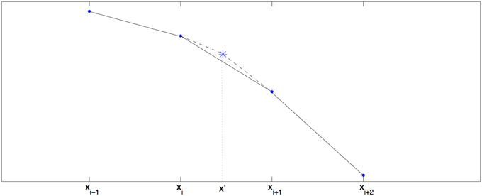
Figure 1. Kink, plot of g against x.

We represent G is the form

$\begin{array}{rc}G(x)=G_1(x)+G_2(x),& (4.7)\end{array}$

where

$\begin{array}{l}{G}_1(x)={𝟙}_{[x_i,x^{\prime }]}(x)[g(V_s(x_i))\\ +\frac{(r-r_F-(1-R_B)\lambda )H_B-g(V_s(x_i))}{x^{\prime }-x_i}(x-x_i)]& (4.8)\end{array}$

$\begin{array}{l}{G}_2(x)={𝟙}_{[x^{\prime },x_{i+1}]}(x)[(r-r_F+(1-R_B)\lambda )H_B\\ +\frac{g(V_s(x_{i+1}))-(r-r_F+(1-R_B)\lambda )H_B}{x_{i+1}-x^{\prime }}(x-x^{\prime })]& (4.9)\end{array}$

Thus, the corrected g(V(x)) is

$\begin{array}{rc}{g}_{corr}(V(x))=g(V(x))+\Theta (x),& (4.10)\end{array}$

where the correction Θ is given by

$\begin{array}{rc}\Theta (x)={𝔼}^x\left[e^{-r\Delta }G(X_{\Delta })\right]=\frac{1}{2\pi }{\displaystyle {\int }_{\text{Im}\xi =\omega }}{e}^{ix\xi -\Delta (r+\psi (\xi ))}Ĝ(\xi )d\xi .& (4.11)\end{array}$

The Fourier transform of Ĝ(ξ) is easy to calculate

$\begin{array}{cc}\widehat{G}(\xi )={{\displaystyle \int }}_{-\infty }^{\infty }{e}^{-ix\xi }G(x)dx=\widehat{G_1}(\xi )+\widehat{G_2}(\xi )& (4.12)\end{array}$

$\begin{array}{cc}\begin{array}{l}\widehat{G_1}(\xi )=-\frac{1}{i\xi }(a{x}^{\prime }+b)e^{-i{x}^{\prime }\xi }+\frac{1}{i\xi }(a{x}_i+b)e^{-i{x}_i\xi }\\ +\frac{a}{{\xi }^2}(e^{-i{x}^{\prime }\xi }-e^{-i{x}_i\xi }),\end{array}& (4.13)\end{array}$

$\begin{array}{l}\widehat{G_2}(\xi )=-\frac{1}{i\xi }(c{x}_{i+1}+d)e^{-i{x}_{i+1}\xi }+\frac{1}{i\xi }(c{x}^{\prime }+d)e^{-i{x}^{\prime }\xi }\\ +\frac{c}{{\xi }^2}(e^{-i{x}_{i+1}\xi }-e^{-i{x}^{\prime }\xi }),& (4.14)\end{array}$

where

$\begin{array}{rcll}a& =& \frac{(r-r_F-(1-R_B)\lambda )H_B-g(V_s(x_i))}{x^{\prime }-x_i},& (4.15)\end{array}$

$\begin{array}{rcll}b& =& g(V_s(x_i))-\frac{(r-r_F-(1-R_B)\lambda )H_B-g(V_s(x_i))}{x^{\prime }-x_i}{x}_i,& (4.16)\end{array}$

$\begin{array}{rcll}c& =& \frac{g(V_s(x_{i+1}))-(r-r_F-(1-R_B)\lambda )H_B}{x_{i+1}-x^{\prime }},& (4.17)\end{array}$

$\begin{array}{l}d=(r-r_F-(1-R_B)\lambda )H_B\\ -\frac{g(V_s(x_{i+1}))-(r-r_F-(1-R_B)\lambda )H_B}{x_{i+1}-x^{\prime }}{x}^{\prime }.& (4.18)\end{array}$

5. Algorithms

In this section, we formulate explicit algorithms for calculation of prices of European options, down-and-out barrier put options and down-and-in first-touch digital options. The algorithms are similar to the ones in [48] with natural modifications to account for the nonlinearity of the stream g(V) and kinks. The underlying is modeled as $S_t=e^{X_t}$, where X_t is a Lévy process of exponential type (λ₋, λ₊), with λ₋ < −1 < 0 < λ₊. The detailed algorithms are as follows:

(1) One must describe the market by giving the riskless rate r > 0 and a formula for the characteristic exponent, ψ(ξ), of the process X. The EMM condition, r + ψ(−i) = 0, must hold if the underlying does not pay dividends. If the dividends are paid at constant rate δ > 0, then the EMM condition becomes r + ψ(−i) = δ.

(2) One must specify the collateral rate, unsecured funding rate, default intensity, recovery rate and collateral thresholds.

(3) One must specify the maturity date, T, and the barrier, H, of the option. In the case of a barrier option, one must also specify its strike price, K > H.

(4) We will use Carr's randomization in the situation where the maturity period, [0, T], of the option is divided into subintervals of equal lengths Thus we only need to specify the number, N, of time steps. Set Δ_t = T∕N and $q=r+{\Delta }_t^{-1}$.

These steps constitute the input of the initial data for the algorithms. The algorithms consist of blocks borrowed from Boyarchenko and Levendorskiĭ [48, 51] with the addition of blocks that account for the non-linearity of additional terms and the new trick which takes the kinks into account, and which is necessary for accurate calculations. From now on we will write V(x) = V_N(x) for the Carr randomization approximation to the value function of the option, calculated using the procedure described in Section 3.2.2 (for an European option) or Section 3.2.1 (for a down-and-out barrier option) or Section 3.2.3 (for a first-touch digital option). The next steps of the algorithm deal are the choice of the parameters of the numerical scheme and auxiliary calculations.

(5) Choose a uniformly spaced grid $\overrightarrow{x}={(x_j)}_{j=1}^M$, where x_j = x₁+(j − 1)Δ and Δ > 0. This is the grid of points where the values of V(x) will be calculated. For European options, we choose x₁ = −MΔ∕2. For barrier options, our algorithm is organized in such a way that the optimal choice of x₁ is h = ln H. (Note that there is no need to calculate V(x) for x < h, because V ≡ 0 on (−∞, h] for a down-and-out barrier option, and V ≡ 1 on (−∞, h] for a down-and-in first-touch digital option).

(6) Set ζ = 2π∕(MΔ) and choose positive integers M₂, M₃ so that the dual grid

$\overrightarrow{\xi }={({\xi }_k)}_{k=1}^{M_1},{\xi }_k=-M_1{\zeta }_1∕2+(k-1){\zeta }_1,$

where M₁ = M · M₂ · M₃ and ζ₁ = ζ∕M₂, is sufficiently long and sufficiently fine. Since one of the subsequent steps uses FFT for arrays of length 2M₁, we recommend making the choices so that M, M₂ and M₃ are powers of 2.

(7) Calculate the values of ${\varphi }_q^{+}(\xi )$ on the grid $\overrightarrow{\xi }$ using the algorithm of Section A.1.1. Then find the values of ${\varphi }_q^{-}(\xi )$ on $\overrightarrow{\xi }$ using the identity ${\varphi }_q^{+}(\xi ){\varphi }_q^{-}(\xi )=q{(q+\psi (\xi ))}^{-1}$.

(8) Calculate the convolution coefficients $c_{\ell }^0,c_{\ell }^1,c_{\ell }^{\Delta },c_{-,\ell }^1,c_{\ell }^{-}$ used for the enhanced realization of the operators ${{ℰ}}_q$ (see Section 4.4.1) and ${{ℰ}}_q^{-}$ (see Section 4.4.3).

To complete the calculation of prices using Carr's randomization procedure, we must now consider the three types of options separately. At each step below, the inputs are function values on the chosen grid, and the output are the values of another function at the same grid. For simplicity, we write x instead of a generic point x_j on the grid.

5.1. Pricing European Options

The remaining steps are as follows:

(8) Set V₀(x_j) = G(x_j) for each j, where G is the payoff function such as European call/put or digitals.

(9) For s = 0, 1, …, N − 1, calculate the nonlinear stream g(V_s(x_j)) and its correction using the procedures in 4.5 then

$\begin{array}{l}{f}_s(x)={\Delta }_s^{-1}{V}_s(x)+g(V_s(x)),\\ V_{s+1}(x)=q_s^{-1}{{ℰ}}_q{f}_s(x).\end{array}$

(10) The vector V_N is the approximation to the value function of the European option, at points of the chosen grid.

5.2. Pricing Down-and-Out Barrier Put Options

For a down-and-out barrier put options, the remaining steps are as follows:

(8) For 1 ≤ s ≤ N, put

$W_s(x)={𝟙}_{[h,+\infty )}(x)·({{ℰ}}_q^{+}{V}_{s-1})(x),$

where h = ln H (and H is the barrier for the option). For s = 0, set $V_0(x)={𝟙}_{[h,+\infty )}(x){(K-e^x)}_{+}$ where h = ln H. Then calculate the Fourier transform of V₀:

$\widehat{V_0}(x)=K·\frac{e^{-i\xi h}-e^{-i\xi lnK}}{i\xi }+\frac{e^{(1-i\xi )h}-e^{(1-i\xi )lnK}}{1-i\xi }.$

For 0 ≤ s ≤ N − 1, we have

$W_{s+1}(x)={𝟙}_{[h,+\infty )}(x)·({{ℰ}}_{q_s}^{+}{f}_s)(x),$

where f_s(x) = q_sW_s(x) − g(W_s(x)). Then calculate the auxiliary function W₁(x) on the x-grid:

$W_1(x)={𝟙}_{[h,+\infty )}(x)·{{ℱ}}_{\xi \to x}^{-1}\left({\varphi }_{q_0}^{+}(\xi )·\widehat{V_0}(x)\right).$

(9) In the cycle for s = 0, …, N − 3, N − 2, calculate the values of W_s(x) on the x-grid using the EPV operator ${{ℰ}}_{q_s}$ and the following formula:

$W_{s+1}(x)=q_s^{-1}·{𝟙}_{[h,+\infty )}(x)·({{ℰ}}_{q_s}{f}_s)(x).$

Calculate the correction for g and set

$f_s(x)={\Delta }_s^{-1}{W}_s(x)+g(W_s(x)).$

(10) For s = N, compute the value of V(x) on the x-grid using the EPV operator ${{ℰ}}_q^{-}$ and the formula

$V_N(x)=q_{N-1}^{-1}·({ℰ}_{q_{N-1}}^{-}{f}_{N-1})(x)$

The vector V_N is the desired approximation to the value function of the down-and-out barrier put option.

5.3. Pricing Down-and-In First Touch Digitals

For down-and-in first touch digital options, it is convenient to work with the auxiliary function U_s(x) = 1 − V_s(x), and the remaining steps are as follows:

(8) For s = 0, set V₀(x) = 𝟙_{[h, +∞)}(x) where h = ln H. For 0 ≤ s ≤ N − 1, we define U_s(x) = 1 − V_s(x) and set

$W_{s+1}(x)={𝟙}_{[h,+\infty )}(x)·({{ℰ}}_{q_s}^{+}{U}_s)(x).$

Calculate

$W_1(x)={𝟙}_{[h,+\infty )}(x)·{{ℰ}}_q({𝟙}_{[h,+\infty )}(x))$

(9) In the cycle for s = 2, …, N − 3, N − 1, calculate the values of W_s(x) on the x-grid using the EPV operator ${{ℰ}}_{q_s}$ and the following formula:

$W_{s+1}(x)=q_s^{-1}·{𝟙}_{[h,+\infty )}(x)·{{ℰ}}_{q_s}(f_s(x)+q_s^{-1}·{𝟙}_{[h,+\infty )}(x)),$

where f_s(x) = q_sW_s(x) − g(1 − W_s(x)). Calculate the correction for g and set

$f_s(x)={\Delta }_s^{-1}{W}_s(x)+g(W_s(x)).$

(10) For s = N, compute the value of V(x) on the x-grid using the EPV operator ${{ℰ}}_q^{-}$ and the formula

$\begin{array}{l}{W}_N(x)=q_{N-1}^{-1}·{𝟙}_{[h,+\infty )}(x)·{{ℰ}}_{q_{N-1}}^{-}(f_{N-1}(x)+q_{N-1}^{-1}\\ ·{𝟙}_{[h,+\infty )}(x))\\ V_N(x)=1-W_N(x)\end{array}$

The vector V_N is the desired approximation to the value function of the down-and-in first touch digital option.

6. Numerical Examples

All calculations and the results presented in this paper were performed in MATLAB R2014a, on a computer with processor Intel Core i5 (2.7 GHz), memory 8 GB 1600 MHz DDR3, under the Mac OS X 10.9.4 operating system. The tables are collected in Appendix C.1.

We calibrate some of the models to June 2015 put options on the Hang Seng index as of 9 January 2015. Namely, we calibrate the market data to the DEJD, KoBoL, VG and NIG models. We use the algorithms in Section 5 to calculate prices for European options, down-and-out barrier put options and down-and-in first touch digital options for these models. As one may expect the trade volume should be better when the option is close to maturity, say less than 1 month. Hence we then use the same procedures to re-calibrate the models again to June 2015 put options on the Hang Seng Index as of 28 May 2015 and price the options with adjustments. We observe that when the time to maturity decreases, the total adjustments become similar across different models but the linearization errors remain.

Prices and adjustments for European options are presented in Tables 1, 2, the models are calibrated to give (approximately) the same at-the-money put option prices in order to compare the adjustments for each models. One can observe that the adjustments are quite close for BM, VG and NIG, while the total adjustments for DEJD and KoBoL are larger for data as of 9 January 2015. For data as of 28 May 2015, the total adjustments are similar for the models considered except KoBoL. We have mentioned at the beginning of the paper that it is impossible to separate effects of CVA and FVA due to nonlinearity of the pricing problem. We observe that the error of separating CVA and FVA is significant and up to 30% in the DEJD and KoBoL model on 9 January and 50% in the KoBoL model on 28 May 2015.The prices and adjustments for European options for KoBoL are computed for different initial spot price using data as of 9 January and 28 May (Tables 3, 4 respectively).The plot of prices and adjustments against spot are in Figure 2 using 9 January data where prices with adjustments and without adjustments are plot on the same graph. Prices and adjustments for digital options are presented in Tables 5, 6. One can observe that the adjustments are similar for all of the models under consideration in both sets of data. In Tables 7, 8, we show the prices and adjustments for digital options under KoBoL computed for different initial spot prices and the plot of prices and adjustments against spot are in Figure 3.

TABLE 1

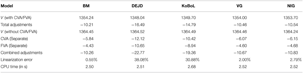
Table 1. Prices of at-the-money European put for different models as of 9 January 2015, time to maturity T = 0.463, spot, strike S = K = 24,000, risk-free rate r = 0.52%, collateral rate r_C = 1%, funding rate r_F = 1.7% default intensity λ = 0.05, recovery rate R_B = 0.4, collateral threshold H_B = 500.

TABLE 2

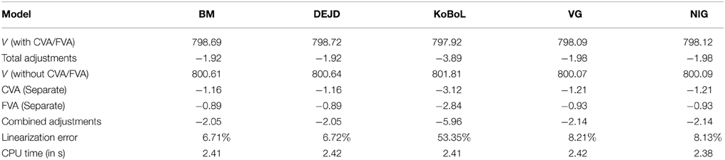
Table 2. Prices of at-the-money European put for different models as of 28 May 2015, time to maturity T = 0.0877, spot S = 27,454.31, strike K = 27,400, risk-free rate r = 0.25%, collateral rate r_C = 1%, funding rate r_F = 1.7% default intensity λ = 0.05, recovery rate R_B = 0.4, collateral threshold H_B = 500.

TABLE 3

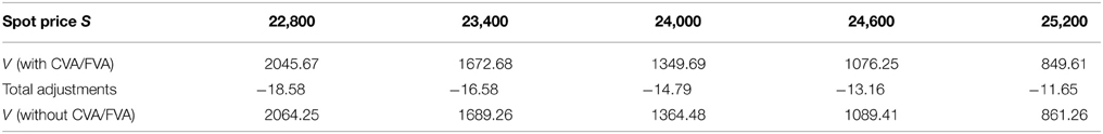
Table 3. Prices of European put under KoBoL process as of 9 January 2015, time to maturity T = 0.463, strike K = 24,000, risk-free rate r = 0.52%, collateral rate r_C = 1%, funding rate r_F = 1.7% default intensity λ = 0.05, recovery rate R_B = 0.4, collateral threshold H_B = 500, CPU time: 2.68 s.

TABLE 4

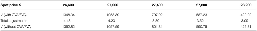
Table 4. Prices of European put under KoBoL process as of 28 May 2015, time to maturity T = 0.0877, strike K = 27,400, risk-free rate r = 0.25%, collateral rate r_C = 1%, funding rate r_F = 1.7% default intensity λ = 0.05, recovery rate R_B = 0.4, collateral threshold H_B = 500, CPU time: 2.68 s.

FIGURE 2

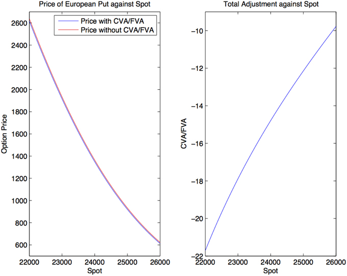
Figure 2. Prices of European put under KoBoL process as of 9 January 2015, time to maturity T = 0.463, strike K = 24,000, risk-free rate r = 0.52%, collateral rate r_C = 1%, funding rate r_F = 1.7% default intensity λ = 0.05, recovery rate R_B = 0.4, collateral threshold H_B = 500.

TABLE 5

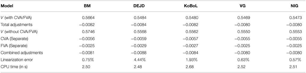
Table 5. Prices of at-the-money digital put for different models as of 9 January 2015, time to maturity T = 0.463, spot, strike S = K = 24,000, risk-free rate r = 0.52%, collateral rate r_C = 1%, funding rate r_F = 1.7% default intensity λ = 0.05, recovery rate R_B = 0.4, collateral threshold H_B = 0.5.

TABLE 6

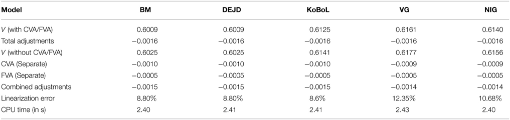
Table 6. Prices of at-the-money digital put for different models as of 28 May 2015, time to maturity T = 0.0877, spot S = 27,454.31, strike K = 27,400, risk-free rate r = 0.25%, collateral rate r_C = 1%, funding rate r_F = 1.7% default intensity λ = 0.05, recovery rate R_B = 0.4, collateral threshold H_B = 500.

TABLE 7

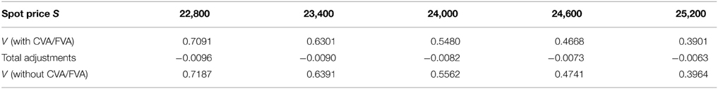
Table 7. Prices of digital put under KoBoL process as of 9 January 2015, time to maturity T = 0.463, spot, strike S = K = 24,000, risk-free rate r = 0.52%, collateral rate r_C = 1%, funding rate r_F = 1.7% default intensity λ = 0.05, recovery rate R_B = 0.4, collateral threshold H_B = 0.5, CPU time: 2.68 s.

TABLE 8

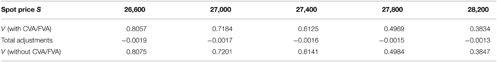
Table 8. Prices of digital put under KoBoL process as of 28 May 2015, time to maturity T = 0.0877, strike K = 27,400, risk-free rate r = 0.25%, collateral rate r_C = 1%, funding rate r_F = 1.7% default intensity λ = 0.05, recovery rate R_B = 0.4, collateral threshold H_B = 500, CPU time: 2.41 s.

FIGURE 3

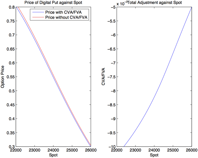
Figure 3. Prices of digital put under KoBoL process as of 9 January 2015, time to maturity T = 0.463, spot, strike S = K = 24,000, risk-free rate r = 0.52%, collateral rate r_C = 1%, funding rate r_F = 1.7% default intensity λ = 0.05, recovery rate R_B = 0.4, collateral threshold H_B = 0.5.

Prices and adjustments for down-and-out put options are presented in Tables 9, 10. We observe that the error of separating CVA and FVA have little impact on down-and-out put options while the adjustments vary for different models for both sets of data. The prices and adjustments for down-and-out put options under KoBoL are computed for different initial spot prices (see Tables 11, 12). Prices and adjustments for first touch digital options are presented in Tables 13, 14. We observe that the error of separating CVA and FVA have significant impact for the models under consideration on the data as of 9 January 2015. The prices and adjustments for first touch digital under KoBoL are computed for different initial spot prices (Tables 15, 16).

TABLE 9

Table 9. Prices of at-the-money down-and-out put for different models as of 9 January 2015, time to maturity T = 0.463, spot, strike S = K = 24,000, barrier H = 23,500, risk-free rate r = 0.52%, collateral rate r_C = 1%, funding rate r_F = 1.7% default intensity λ = 0.05, recovery rate R_B = 0.4, collateral threshold H_B = 0.1.

TABLE 10

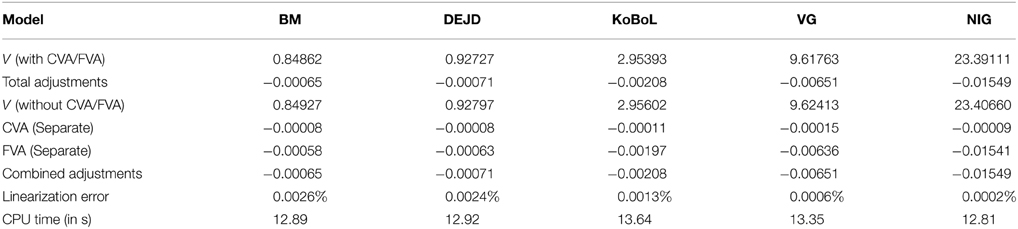
Table 10. Prices of at-the-money down-and-out put for different models as of 28 May 2015, time to maturity T = 0.0877, spot S = 27,454.31, strike K = 27,400, barrier H = 27,000, risk-free rate r = 0.25%, collateral rate r_C = 1%, funding rate r_F = 1.7% default intensity λ = 0.05, recovery rate R_B = 0.4, collateral threshold H_B = 0.1.

TABLE 11

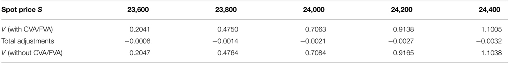
Table 11. Prices of down-and-out put under KoBoL process as of 9 January 2015, time to maturity T = 0.463, spot, strike S = K = 24,000, barrier H = 23,500, risk-free rate r = 0.52%, collateral rate r_C = 1%, funding rate r_F = 1.7% default intensity λ = 0.05, recovery rate R_B = 0.4, collateral threshold H_B = 0.1, CPU time: 16.70 s.

TABLE 12

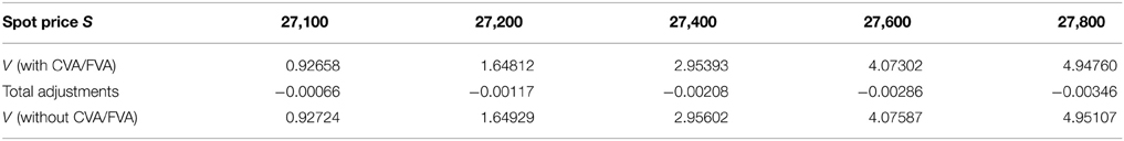
Table 12. Prices of down-and-out put under KoBoL process as of 28 May 2015, time to maturity T = 0.0877, spot S = 27,454.31, strike K = 27,400, barrier H = 27,000, risk-free rate r = 0.25%, collateral rate r_C = 1%, funding rate r_F = 1.7% default intensity λ = 0.05, recovery rate R_B = 0.4, collateral threshold H_B = 0.1, CPU time: 16.64 s.

TABLE 13

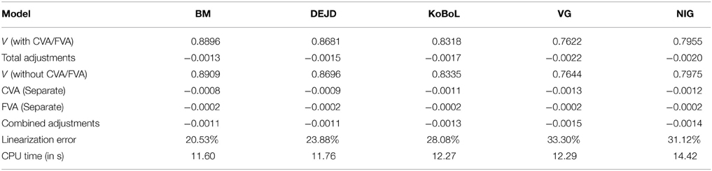
Table 13. Prices of first-touch digitial for different models as of 9 January 2015, time to maturity T = 0.463, spot S = 24,000, barrier H = 23,500, risk-free rate r = 0.52%, collateral rate r_C = 1%, funding rate r_F = 1.7% default intensity λ = 0.05, recovery rate R_B = 0.4, collateral threshold H_B = 0.5.

TABLE 14

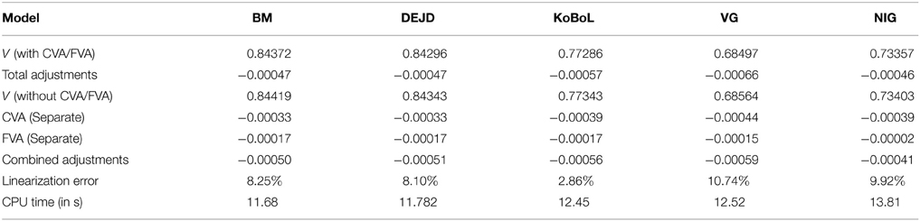
Table 14. Prices of first-touch digitial for different models as of 28 May 2015, time to maturity T = 0.0877, spot S = 27,454.31, barrier H = 27,000, risk-free rate r = 0.25%, collateral rate r_C = 1%, funding rate r_F = 1.7% default intensity λ = 0.05, recovery rate R_B = 0.4, collateral threshold H_B = 0.5.

TABLE 15

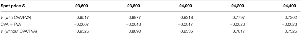
Table 15. Prices of first-touch digital under KoBoL as of 9 January 2015, time to maturity T = 0.463, barrier H = 23,500, risk-free rate r = 0.52%, collateral rate r_C = 1%, funding rate r_F = 1.7% default intensity λ = 0.05, recovery rate R_B = 0.4, collateral threshold H_B = 0.5, CPU time: 12.27 s.

TABLE 16

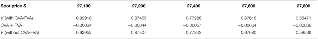
Table 16. Prices of first-touch digital under KoBoL as of 28 May 2015, time to maturity T = 0.0877, barrier H = 27,000, risk-free rate r = 0.25%, collateral rate r_C = 1%, funding rate r_F = 1.7% default intensity λ = 0.05, recovery rate R_B = 0.4, collateral threshold H_B = 0.5, CPU time: 12.45 s.

7. Conclusion

In this paper, we generalized the model of Piterbarg [1] to include (1) the bilateral default risk as in Burgard and Kjaer [2], and (2) jumps in the dynamics of the underlying asset. We use very general Lévy processes of exponential type. We calculate prices for European options, barrier options under general classes of Lévy processes taking CVA and FVA into account simultaneously. We develop an efficient algorithm using the Carr's randomization and Wiener-Hopf factorization to solve the arising non-linear problem. We produce numerical examples which show that the independent calculation of effects of CVA and FVA can result in sizable errors in derivative valuation due to non-linearity of the pricing problem.

The limitations of the method developed in this paper is that portfolio netting effects cannot be modeled using the single model. While this deal-by-deal approach allows traders to access the impact of CVA/FVA for intra-day trading immediately. A possible extension of the current method is to introduce stochastic interest rate into consideration which remains for the future.

Since the financial crisis of 2008, there has been a regulatory drive towards better recognition and mitigation of derivative counterparty credit risk. Basel 3 (as implemented in law as CRD IV in Europe) introduced CVA and CVA risk capital which requires banks to include CVA in derivative valuation based on the market implied default probabilities (from CDS spreads) of the counterparty, and capitalize the additional volatility of derivative valuation due to fluctuation of CDS spreads. The Dodd-Frank Act and EMIR requires standardized derivative contracts to be traded with CCPs under robust collateral agreements. The Basel committee introduced mandatory exchange of initial and variation margins (making the collateral requirements similar to a CCP trade) for all OTC derivative transactions, whilst liquidity coverage ratios introduced in Basel 3 explicitly capture contingent liquidity requirements from derivative transactions. The combined effect of the above is that

• some counterparty credit risk will be transformed into funding risk (the need to fund margin calls), and therefore derivative valuation must incorporate both CVA and FVA simultaneously;

• the remaining counterparty credit risk will largely be driven by gap events, either through jumps in the underlying asset prices or the jump-to-default of a counterparty making it important to incorporate jumps in asset price dynamics in derivative valuation.

The present work is therefore extremely relevant in the context of current industry development and we see potential application of our work in:

• investigating the combined effects of counterparty credit risk and collateral funding costs, particularly in the context of a centralized CVA/FVA desk quantifying the impact of jumps in asset prices when evaluating CVA and/or FVA;

• calculating the upper bound (as portfolio netting effects cannot be modeled using this single model) of the CVA/FVA adjustment for intra-day trading or for valuing particularly large transactions where portfolio netting may be reasonably ignored.

Conflict of Interest Statement

The authors declare that the research was conducted in the absence of any commercial or financial relationships that could be construed as a potential conflict of interest.

Acknowledgments

We thank the participants of SIAM FM 2014, Chicago, November 2014, and especially Tomasz Bielecki and Harvey Sturm for valuable comments and suggestions. The suggestions made by two reviewers are especially appreciated.

Footnotes

1. ^In the formulas below, and elsewhere in the text, we use the standard convention that z^ν = e^{ν·ln z} for any ν ∈ ℂ and any z ∈ ℂ such that z ∉ (−∞, 0]. In turn, ln z denotes the unique branch of the natural logarithm function defined on the complex plane with the negative real axis (−∞, 0] removed, determined by the requirement that ln(1) = 0.

2. ^What we present is not the most common way of writing the formula. Rather, we chose an expression that is equivalent to the standard one and makes the analogy with Equation (2.10) transparent.

References

1. Piterbarg V. Funding beyond discounting: collateral agreements and derivatives pricing. Risk (2010) 2:97–102.

Google Scholar

2. Burgard C, Kjaer M. The FVA Debate - In Theory and Practice (2012). Available online at: http://ssrn.com/abstract=2157634

3. Pykhtin M, Zhu S. A guide to modelling counterparty credit risk. GARP Risk Rev. (2007) 16–22.

4. Brigo D, Buescu C, Morini M. Impact of the first to default time on bilateral CVA. arXiv:11063496. (2011).

Google Scholar

5. Brigo D, Capponi A, Pallavicini A, Papatheodorou V. Collateral Margining in Arbitrage-Free Counterparty Valuation Adjustment Including Re-Hypotecation and Netting (2011). Availble online at: http://ssrn.com/abstract=1744101

6. Brigo D, Morini M. Dangers of Bilateral Counterparty Risk: The Fundamental Impact of Closeout Conventions (2010). Availble online at: http://ssrn.com/abstract=1709370

7. Gregory J. Being two-faced over counterparty credit risk? Risk (2009) 22:86–90.

Google Scholar

8. Gregory J. Counterparty Credit Risk: The New Challenge for Global Financial Markets. West Sussex: Wiley (2010).

Google Scholar

9. Lipton A, Savescu I. CDSs, CVA and DVA – A structural approach. Risk (2013) 26:60–5.

Google Scholar

10. Lipton A, Savescu I. Pricing credit default swaps with bilateral value adjustments. Quant Finance (2014) 14:171–88. doi: 10.1080/14697688.2013.828239

CrossRef Full Text | Google Scholar

11. Lipton A, Sepp A. Credit value adjustment for credit default swaps via the structural default model. J Credit Risk (2009) 5:123–46.

Google Scholar

12. Lipton A, Shelton D. Single- and multi-name credit derivatives: theory and practice. In: Lipton A, Rennie A, editors. The Oxford Handbook of Credit Derivatives. Oxford: Oxford University Press (2011). p. 196–256. doi: 10.1093/oxfordhb/9780199546787.001.0001

CrossRef Full Text

13. Lipton A, Rennie A. The Oxford Handbook of Credit Derivatives. Oxford: Oxford University Press (2011).

Google Scholar

14. Hull J, White A. Valuing derivatives: funding value adjustments and fair value. Financ Anal J. (2014). doi: 10.2139/ssrn.2245821

CrossRef Full Text | Google Scholar

15. Castagna A. Yes, FVA is a Cost for Derivatives Desks - A Note on 'Is FVA a Cost for Derivatives Desks?' by Prof. Hull and Prof. White (2012). Available online at: http://ssrn.com/abstract=2141663

16. Burgard C, Kjaer M. A Generalised CVA with Funding and Collateral (2012). Available online at: http://ssrn.com/abstract=2027195

17. Burgard C, Kjaer M. Partial differential equation representations of derivatives with bilateral counterparty risk and funding costs. J Credit Risk (2012) 7:75–93. doi: 10.2139/ssrn.1605307

CrossRef Full Text | Google Scholar

18. Lu D, Juan F. Credit Value Adjustment and Funding Value Adjustment All Together Adjustment and Funding Value Adjustment All Together (2011). Availble online at: http://ssrn.com/abstract=1803823

19. Wu L. CVA and FVA to Derivatives Trades Collateralized by Cash (2014). Availble online at: http://ssrn.com/abstract=2211347

20. Brigo D, Liu Q, Pallavicini A, Sloth D. Nonlinear valuation under collateral, credit risk and funding costs: a numerical case study extending black-scholes. Handb Fixed-Income Securit. (2014).

Google Scholar

21. Brigo D, Buescu C, Pallavicini A, Liu Q. llustrating a Problem in the Self-Financing Condition in Two 2010-2011 Papers on Funding, Collateral and Discounting (2012). Availble online at: http://ssrn.com/abstract=2103121

22. Pallavicini A, Perini D, Brigo D. Funding Valuation Adjustment: A Consistent Framework Including CVA, DVA, Collateral, Netting Rules and Re-hypothecation (2011). Availble online at: http://ssrn.com/abstract=1969114

23. Brigo D, Pallavicini A. CCPs, Central Clearing, CSA, Credit Collateral and Funding Costs Valuation FAQ: Re-hypothecation, CVA, Closeout, Netting, WWR, Gap-Risk, Initial and Variation Margins, Multiple Discount Curves, FVA? (2013). Availble online at: http://ssrn.com/abstract=2361697

24. Pallavicini A, Perini D, Brigo D. Funding, Collateral and Hedging: Uncovering the Mechanics and the Subtleties of Funding Valuation Adjustments (2012). Availble online at: http://arxiv.org/pdf/1210.3811.pdf

25. Brigo D, Pallavicini A. CCP Cleared or Bilateral CSA Trades with Initial/Variation Margins Under Credit, Funding and Wrong-Way Risks: A Unified Valuation Approach (2014). Availble online at: http://ssrn.com/abstract=2380017

26. Brigo D. Counterparty Risk FAQ: Credit VaR, PFE, CVA, DVA, Closeout, Netting, Collateral, Re-Hypothecation, WWR, Basel, Funding, CCDS and Margin Lending (2012). Availble online at: http://ssrn.com/abstract=1955204

27. Kenyon C, Stamm R. Discounting, LIBOR, CVA and Funding: Interest Rate and Credit Pricing. Palgrave Macmillan (2012). doi: 10.1057/9781137268525

CrossRef Full Text | Google Scholar

28. Antonov A, Bianchetti M, Mihai I. Funding Value Adjustment for General Financial Instruments - Theory and Practice (2013). Availble online at: http://ssrn.com/abstract=2290987

29. Sun W, Rachev S, Fabozzi F. A new approach of using lévy processes for determining high-frequency value at risk predictions. Euro Financ Manag. (2009) 15:340–61. doi: 10.1111/j.1468-036X.2008.00467.x

CrossRef Full Text | Google Scholar

30. Boyarchenko S, Levendorskiĭ S. Non-Gaussian Merton-Black-Scholes Theory. Singapore: World Scientific (2002).

31. Black F, Scholes M. The pricing of options and corporate liabilites. J Polit Econ. (1973) 81:637–59. doi: 10.1086/260062

CrossRef Full Text | Google Scholar

32. Merton RC. Option pricing when underlying stock returns are discontinuous. J Financ Econ. (1976) 3:125–44. doi: 10.1016/0304-405X(76)90022-2

CrossRef Full Text | Google Scholar

33. Lipton A. Assets with jumps. Risk (2002) 149–53.

34. Levendorskiĭ S. Pricing of the American Put under Lévy Processes (2002). Research Report MaPhySto, Aarhus. Available online at http://www.maphysto.dk/publications/MPS-RR/2002/44.pdf

35. Levendorskiĭ S. Levendorskiĭ S. Pricing of the american put under lévy processes. Int J Theor Appl Finance (2004) 7:303–35. doi: 10.1142/S0219024904002463

CrossRef Full Text | Google Scholar

36. Lipton A. Path-Dependent Options on Assets with Jumps (2002). In: 5^th Columbia-Jaffe Conference. Available online at: http://www.math.columbia.edu/~lrb/columbia2002.pdf

37. Kou S. A jump-diffusion model for option pricing. Manag Sci. (2002) 48:1086–101. doi: 10.1287/mnsc.48.8.1086.166

CrossRef Full Text | Google Scholar

38. Koponen I. Analytic approach to the problem of convergence of truncated lévy flights towards the gaussian stochastic process. Phys Rev. (1995) 52:1197–9. doi: 10.1103/physreve.52.1197

PubMed Abstract | CrossRef Full Text | Google Scholar

39. Boyarchenko S, Levendorskiĭ S. Option pricing for truncated lévy processes. Int J Theor Appl Finance (2000) 3:549–52. doi: 10.1142/S0219024900000541

CrossRef Full Text | Google Scholar

40. Carr P, Geman H, Madan DB, Yor M. The fine structure of asset returns: an empirical investigation. J Bus. (2002) 75:305–32. doi: 10.1086/338705

CrossRef Full Text | Google Scholar

41. Madan DB, Seneta E. The variance gamma (V.G.) model for share market returns. J Bus. (1990) 63:511–24. doi: 10.1086/296519

CrossRef Full Text | Google Scholar

42. Madan DB, Seneta E. Option pricing with V.G. martingale components. Math Finance (1991) 1:39–55. doi: 10.1111/j.1467-9965.1991.tb00018.x

CrossRef Full Text | Google Scholar

43. Madan DB, Carr P, Chang EC. The variance gamma process and option pricing. Eur Finance Rev. (1998) 2:79–105. doi: 10.1023/A:1009703431535

CrossRef Full Text | Google Scholar

44. Barndorff-Nielsen OE. Processes of normal inverse gaussian type. Finance Stochast. (1998) 2:41–68. doi: 10.1007/s007800050032

CrossRef Full Text | Google Scholar

45. Kuznetsov A. Wiener-hopf factorization and distribution of extrema for a family of lévy processes. Ann Appl Probabil. (2010) 20:1801–30. doi: 10.1214/09-AAP673

CrossRef Full Text | Google Scholar

46. Kuznetsov A, Kyprianou AE, Pardo JC. Meromorphic lévy processes and their fluctuation identities. Ann Appl Probabil. (2012) 22:1101–35. doi: 10.1214/11-AAP787

CrossRef Full Text | Google Scholar

47. Boyarchenko S, Levendorskiĭ S. Irreversible Decisions under Uncertainty. New York: Springer (2007).

Google Scholar

48. Boyarchenko M, Levendorskiĭ S. Prices and sensitivities of barrier and first-touch digital options in lévy-driven models. Int J Theor Appl Finance (2009) 12:1125–70. doi: 10.1142/S0219024909005610

CrossRef Full Text | Google Scholar

49. Carr P. Randomization and the American put. Rev Financ Stud. (1998) 11:597–626. doi: 10.1093/rfs/11.3.597

CrossRef Full Text | Google Scholar

50. Boyarchenko S, Levendorskiĭ S. Barrier options and touch-and-out options under regular lévy processes of exponential type. Ann Appl Probabil. (2002) 12:1261–98. doi: 10.1214/aoap/1037125863

CrossRef Full Text | Google Scholar

51. Boyarchenko M, Levendorskiĭ S. Refined and Enhanced FFT Techniques, With an Application to the Pricing of Barrier Options (2008). Availbale online at: http://ssrn.com/abstract=1142833

52. Sato K. Lévy Processes and Infinitely Divisible Distributions. Cambridge: Cambridge University Press (1999).

Google Scholar

53. Asmussen S, Avram F, Pistorius MR. Russian and american put options under exponential phase-type lévy models. Stochast Process Appl. (2004) 109:79–111. doi: 10.1016/j.spa.2003.07.005

CrossRef Full Text | Google Scholar

54. Jeannin M, Pistorius MR. A Transform Approach to Calculate Prices and Greeks of Barrier Options Driven By a Class of Lévy Processes (2007). King's College London and Nomura Models and Methodology Group Preprint (2007). Available online at: http://www.mth.kcl.ac.uk/staff/m_pistorius/LevyBarrier.pdf

Appendix A

A.1. Algorithms II

A.1.1. Calculation of the Wiener-Hopf factors

In order to be able to implement the enhanced realization of the operators ${{ℰ}}_q^{\pm }$, we must first know how to calculate the values of the functions ${\varphi }_q^{\pm }(\xi )$ that appear in Equation (4.2). Unfortunately, apart from a few special cases (such as the hyper-exponential Lévy processes [35, 53, 54]), no explicit formulas for ${\varphi }_q^{\pm }(\xi )$ are known. Instead, one must use the integral formulas recalled in Section 4.2. We will not repeat these formulas here, but will only give the discretized versions thereof, after introducing some auxiliary notation.

As before, we consider a uniformly spaced grid of points $\overrightarrow{\xi }={({\xi }_k)}_{k=1}^M$ in ℝ, where ξ_k = ξ₁+(k − 1)ζ for all 1 ≤ k ≤ M and ζ > 0 is fixed. We assume that there exist λ₋ < 0 < λ₊ such that the Lévy process X = {X_t}_t≥0 is of exponential type (λ₋, λ₊), and recall that ψ(ξ) denotes the characteristic exponent of X (see Section 2.2).

We obtain approximate formulas for ${\varphi }_q^{\pm }({\xi }_k)$ using a simplified version of the trapezoidal rule to discretize Equation (4.3). Due to the fact that the integrand in Equation (4.3) decays somewhat slower than |η|⁻² as Re η → ±∞, it is sometimes necessary to use an η-grid that is longer than the ξ-grid for this discretization, in order to guarantee the desired precision of the calculation of ${\varphi }_q^{\pm }({\xi }_k)$.

With these remarks in mind, and with the notation above, we present an algorithm for the approximate calculation of the values ${({\varphi }_q^{\pm }({\xi }_k))}_{k=1}^M$.

• Select a positive integer m that controls the length of the η-grid.

• Choose ω₋ ∈ (λ₋, 0) and ω₊ ∈ (0, λ₊) such that there exists δ > 0 with Re(q + ψ(η)) ≥ δ whenever Im η ∈ [ω₋, ω₊]. As a rule of thumb, we recommend taking ω_± = λ_±∕3 in the algorithms that are based on Carr's randomization method, since in these examples, q is rather large.

• Define the η-grid as follows:

${\overrightarrow{\eta }}^{\pm }={({\eta }_{\ell }^{\pm })}_{\ell =1}^{mM},{\eta }_{\ell }^{\pm }=-mM\zeta ∕2+(\ell -1)\zeta +i{\omega }_{\mp },$

where ${\overrightarrow{\eta }}^{+}$ (resp., ${\overrightarrow{\eta }}^{-}$) is used for the calculation of ${\varphi }_q^{+}$ (resp., ${\varphi }_q^{-}$).

• Using the simplified trapezoid rule to discretize Equation (4.3) leads to the following approximation:

${\varphi }_q^{\pm }({\xi }_k)\approx exp\left[\pm \frac{\zeta ·{\xi }_k}{2\pi i}{\displaystyle \sum _{\ell =1}^{mM}}\frac{ln(1+q^{-1}\psi ({\eta }_{\ell }^{\pm }))}{{\eta }_{\ell }^{\pm }({\xi }_k-{\eta }_{\ell }^{\pm })}\right].$

• The last formula can be rewritten as follows:

$\begin{array}{rc}{\varphi }_q^{\pm }({\xi }_k)\approx exp\left[\pm \frac{\zeta ·{\xi }_k}{2\pi i}{\displaystyle \sum _{j=1}^m}{I}_j({\xi }_k)\right],& (9.1)\end{array}$

where

$I_j({\xi }_k)={\displaystyle \sum _{\ell =1+(j-1)M}^{jM}}\frac{ln(1+q^{-1}\psi ({\eta }_{\ell }^{\pm }))}{{\eta }_{\ell }^{\pm }({\xi }_k-{\eta }_{\ell }^{\pm })},1\le j\le m.$

• Noting that ${\xi }_k-{\eta }_{\ell }^{\pm }=\left({\xi }_1+mM\zeta ∕2-i{\omega }_{\mp }\right)-(k-\ell )\zeta$ depends only on the difference k − ℓ, calculate each of the arrays ${(I_j({\xi }_k))}_{k=1}^M$ for j = 1, 2, …, m using the “fast convolution” algorithm of Section A.1.3.

• Using the results of the previous step, calculate the right hand side of Equation (9.1).

Remark A.1. In practice, it is clearly computationally more efficient to calculate either the values $({\varphi }_q^{+}({\xi }_k))$ or the values $({\varphi }_q^{-}({\xi }_k))$, and then use the analytic form Equation (3.3) of the Wiener-Hopf factorization formula, namely, ${\varphi }_q^{+}(\xi ){\varphi }_q^{-}(\xi )=q{(q+\psi (\xi ))}^{-1}$, to calculate the values $({\varphi }_q^{-}({\xi }_k))$ (respectively, $({\varphi }_q^{+}({\xi }_k)))$.

A.1.2. Convolution Coefficients

The algorithm of calculating the convolution coefficients $c_l^1,c_l^0-c_l^1$ and $c_{\Delta }^l$ using refined inverse fast Fourier transform (rifft) will be given. The rifft procedures follow Boyarchenko and Levendorskiĭ [51].

We present the algorithm for calculating $c_l^0$; the other coefficients $c_l^1,c_l^{\Delta }$ for ${{ℰ}}_q$, $c_{+,l}^0-c_{+,l}^1,c_l^{+}$ for ${{ℰ}}_q^{+}$ and $c_{-,l}^1,c_l^{-}$ for ${{ℰ}}_q^{-}$ can be calculated in the same way as in this section.

We have

$c_l^0=\frac{\Delta }{2\pi }{\displaystyle {\int }_{-\infty }^{\infty }}\frac{q}{q+\psi (\xi )}·\frac{1-e^{-i\xi \Delta }}{i\xi \Delta }·e^{i\xi \Delta }d\xi$

(1) We use the dual grid ${({\xi }_k)}_{k=1}^{M_1}$ constructed in Section 5 to continue the calculations.

(2) Calculate the integrand by

$g({\xi }_k)=\frac{q\Delta }{q+\psi ({\xi }_k)}·\frac{1-e^{-i\xi \Delta }}{i\xi \Delta },$

for points near ξ = 0 (ξ = 0 is a removable singularity), we use power series expansion to calculate the integrand.

(3) For each l = 1, 2, …, M₂, and each j = 1, 2, …, M₃, calculate inverse fast Fourier transform of g on the sub-grid

$\overrightarrow{\xi }(j,l)={({\xi }_{M_2(k-1+(j-1)M)+l})}_{k=1}^{M_2}.$

(4) Finally take the sum

${{ℱ}}_{fast}^{-1}g=\frac{1}{M_2}{\displaystyle \sum _{j=1}^{M_3}}{\displaystyle \sum _{l=1}^{M_2}}{{ℱ}}_{fast}^{-1}(g^{j,l}).$

A.1.3. Fast Convolution

Given array f_j = f(x_j), we want to calculate the sums

$h_k={\displaystyle \sum _{j=1}^M}{f}_j{g}_{k-j}.$

(1) Let $\widetilde{f_j}=\{\begin{array}{l}{f}_j,1\le j\le M\hfill \\ 0,M+1\le j\le 2M\hfill \end{array}$. Then $\tilde{f}$ is a vector of length 2M.

(2) Let $\tilde{g}$ be a vector of length 2M where the entries are

$g_0,g_1,\dots ,g_{M-1},0,g_{1-M},g_{2-M},\dots ,g_{-1}$

(3) Calculate the vector $\tilde{h}={(\widetilde{h_l})}_{l=1}^{2M}$ by

$\tilde{h}=\mathrm{fft}(\tilde{f}){·}^{*}\mathrm{fft}(\tilde{g})$

(4) The sum is

$h_k=\mathrm{ifft}{(\tilde{h})}_k,1\le k\le M.$

Appendix B

B.1. Streams of Payoffs

B.1.1. On-Default Cashflows

Let τ_B, τ_C be the default time of the bank and the counterparty respectively. Define the time of the first default event among the two parties as the stopping time

$\tau :=({\tau }_A\wedge {\tau }_B).$

The close-out amount at default is the costs or losses that the surviving party incurs when replacing the terminated deal with an economic equivalent. The size of these costs will depend on which party survives and we define the close-out amount as

$V_{\tau }:={𝟙}_{\left\{\tau ={\tau }_A<{\tau }_B\right\}}{V}_{B,\tau }+{𝟙}_{\left\{\tau ={\tau }_B<{\tau }_A\right\}}{V}_{A,\tau }$

where V_{B, τ} is the close-out amount on the counterparty's default priced at time τ by the bank and V_{A, τ} is the close-out amount if the bank defaults. We adopt the approach of Brigo [5] Brigo et al. [20] listing and net the exposure against the pre-default value of the collateral. If we aggregate all these cashflows and the pre-default value of collateral account, we obtain the expression for the on-default cashflow

$\begin{array}{l}{\chi }_{\tau }(C,V):={𝟙}_{\left\{\tau ={\tau }_C<{\tau }_B\right\}}(V_{B,\tau }-(1-R_A){(V_{B,\tau }-C_{\tau })}^{+})+\\ {𝟙}_{\left\{\tau ={\tau }_B<{\tau }_C\right\}}(V_{C,\tau }-(1-R_B){(V_{C,\tau }-C_{\tau })}^{-})\end{array}$

If both parties agree on the exposure, that is V_{B, τ} = V_{C, τ} = V_τ, when we take the risk-neutral expectation, we see that the price of the discounted on-default cashflow,

$\begin{array}{l}{𝔼}_t\left[{𝟙}_{\left\{t<\tau <T\right\}}D(t,\tau ){\chi }_{\tau }(C,V)\right]={𝔼}_t\left[{𝟙}_{\left\{t<\tau <T\right\}}D(t,\tau )V_{\tau }\right]\\ -\text{CVA}(t,T;C)+\text{DVA}(t,T;C),\end{array}$

is the present value of the close-out amount reduced by the positive collateralized CVA and DVA and

$\begin{array}{rc}\text{CVA}(t,T;C)& :={𝔼}_t\left[{𝟙}_{\left\{\tau ={\tau }_C<T\right\}}D(t,\tau )(1-R_A){(V_{\tau }-C_{\tau })}^{+}\right]\\ \text{DVA}(t,T;C)& :={𝔼}_t\left[{𝟙}_{\left\{\tau ={\tau }_B<T\right\}}D(t,\tau )(1-R_B){(V_{\tau }-C_{\tau })}^{-}\right]\end{array}$

B.1.2. Stream of Collateral

A margining procedure specifies the set of dates during the life of a deal when both parties post or withdraw collaterals, according to their current exposure, to or from an account held by the collateral taker. A realistic margining practice should allow for collateral posting only on a fixed time-grid {t₁, …, t_n}. Without loss of generality, we assume that the collateral account C_t is held by the bank if C_t > 0, and by the counterparty if C_t < 0.

The CSA agreement holding between the counterparties ensures that the collateral taker remunerates the account at a particular accrual rate. We denote the collateral rate $r_c^{+}(t,T)$ when the collateral are taken by the bank, and $r_c^{+}(t,T)$ if otherwise. The effective collateral rate ${\tilde{r}}_c(t,T)$ is defined as

${\tilde{r}}_c(t,T)=r_c^{-}(t,T){𝟙}_{\left\{C_t<0\right\}}+r_c^{+}(t,T){𝟙}_{\left\{C_t>0\right\}}$

and the corresponding zero-coupon bond

$P^{{\tilde{r}}_c}(t,T)=\frac{1}{1+(T-t){\tilde{r}}_c(t,T)}$

Assume the interests accrued by the collateral are saved into the account itself. The cashflows originating from the bank and going to the counterparty if default events do not occur are

(1) The bank opens the collateral account at the first margin date t₁ if C_t1 < 0 (the counterparty is the collateral taker);

(2) The bank posts to or withdraws from the account at each t_k, as long as C_tk < 0, and the collateral account grow at the CSA rate $r_c^{-}(t_k,t_{k+1})$ between posting dates;

(3) The bank closes the account at the last margining date t_m if C_tm < 0.

On the other hand, the counterparty considers the same cashflows for opposite values of the collateral account at each margining date with the CSA rate $r_c^{+}$. We define the sum of discounted margining cashflows as given by

$\begin{array}{l}\Gamma (t,T;C):\\ ={𝟙}_{\left\{t\le t_1<T\right\}}{C}_{t_1}^{-}D(t,t_1)-{𝟙}_{\left\{t<t_n\le T\right\}}{C}_{t_n}^{-}D(t,t_n)\\ -{\displaystyle \sum _{k=1}^{n-1}}{𝟙}_{\left\{t<t_{k+1}\le T\right\}}\left(\frac{C_{t_k}^{-}}{P_{t_k}^{r_c^{-}}(t_k,t_{k+1})}-C_{t_{k+1}}^{-}\right)D(t,t_{k+1})\\ +{𝟙}_{\left\{t\le t_1<T\right\}}{C}_{t_1}^{+}D(t,t_1)-{𝟙}_{\left\{t<t_n\le T\right\}}{C}_{t_n}^{+}D(t,t_n)\\ -{\displaystyle \sum _{k=1}^{n-1}}{𝟙}_{\left\{t<t_{k+1}\le T\right\}}\left(\frac{C_{t_k}^{+}}{P_{t_k}^{r_c^{+}}(t_k,t_{k+1})}-C_{t_{k+1}}^{+}\right)D(t,t_{k+1})\\ \end{array}$

Let τ be the time of the first default event. To introduce default event, we can stop collateral margining when they occur, so we have

$\gamma (t,T;C):=\Gamma (t,T\wedge \tau ;C)$

where γ is the sum of all (discounted) margining cashflows up to the first default event.

$\gamma (t,T\wedge \tau ;C)={\displaystyle \sum _{k=1}^{n-1}}{𝟙}_{\left\{t\le t_k<(T\wedge \tau )\right\}}D(t,t_k)C_{t_k}\left(1-\frac{P(t_k,t_{k+1})}{P^{{\tilde{r}}_c}(t,t_{k+1})}\right)$

If we use a first order expansion (for small ${\tilde{r}}_c$ and r), we can approximate

$\begin{array}{l}\gamma (t,T\wedge \tau ;C)\approx {\displaystyle \sum _{k=1}^{n-1}{𝟙}_{\{t\le t_k<(T\wedge \tau )\}}}D(t,t_k)C_{t_k}(r(t_k,t_{k+1})\\ -{\tilde{r}}_c(t_k,t_{k+1}))(t_{k+1}-t_k)\end{array}$

By taking the time limit, we have the expression for the stream of the collateral:

$\gamma (t,T\wedge \tau ;C)={\displaystyle {\int }_t^{T\wedge \tau }}(r_s-{\tilde{r}}_c(s))C_{s}D(t,s)ds$

B.1.3. Stream of Funding

Denote F_t the funding account and without loss of generality, we assume that the the trading desk is borrowing from the treasury if F_t > 0, and otherwise lending to treasury if F_t < 0. Similar to the case in collateral, we assume the trading desk enters a funding position on a discrete time-grid {t₁, …, t_m}.

Given two adjacent funding times t_j and t_{j + 1}, for 1 ≤ j ≤ m − 1, the desk enters a position in cash equal to F_tj at time t_j. At time t_{j + 1} the desk redeems the position again and either returns the cash to the treasury if it was a borrowing position and pays the funding costs on the borrowed cash, or it gets the cash back if it was a lending position and receives funding benefits as interest on the invested cash. We assume that these funding costs and benefits are determined at the start date of each funding period and charged at the end of the period.

Let $P^{r_f^{+}}(t,T)$ be the price of a borrowing contract at t where the desk pays one unit of cash at maturity T > t, and let $P^{r_f^{-}}(t,T)$ be the price of a lending contract where the desk receives one unit of cash at maturity. The corresponding accrual rates are given by

$r_f^{\pm }(t,T)=\frac{1}{T-t}\left(\frac{1}{P^{r_f^{\pm }}(t,T)}-1\right)$

In other words, if the desk requires to borrow cash, this can be done at the funding/borrowing rate $r_f^{+}$, while surplus cash can be invested at the lending rate $r_f^{-}$. We define the effective funding rate ${\tilde{r}}_f$ faced by the desk as

${\tilde{r}}_f(t,T)=r_f^{-}(t,T){𝟙}_{F_t<0}+r_f^{+}(t,T){𝟙}_{F_t>0}$

Repeating the similar steps as in the part of collateral, the sum of discounted cashflows from funding is equal to

$\theta (t,T\wedge \tau ;F)={\displaystyle \sum _{j=1}^{m-1}}{𝟙}_{\left\{t\le t_j<(T\wedge \tau )\right\}}D(t,t_j)F_{t_j}\left(1-\frac{P(t_j,t_{j+1})}{P^{{\tilde{r}}_f}(t,t_{j+1})}\right)$

If we use a first order expansion (for small ${\tilde{r}}_f$ and r), we can approximate

$\begin{array}{l}\theta (t,T\wedge \tau ;F)\approx {\displaystyle \sum _{j=1}^{m-1}{𝟙}_{\{t\le t_j<(T\wedge \tau )\}}}D(t,t_j)F_{t_j}(r(t_j,t_{j+1})\\ -{\tilde{r}}_f(t_j,t_{j+1}))(t_{j+1}-t_j)\end{array}$

By taking the time limit, we have the expression for the stream of the collateral:

$\begin{array}{l}\theta (t,T\wedge \tau ;F)={\displaystyle {\int }_t^{T\wedge \tau }}(r_s-{\tilde{r}}_f(s))F_{s}D(t,s)ds\\ ={\displaystyle {\int }_t^{T\wedge \tau }}(r_s-{\tilde{r}}_f(s))(V_s-C_s)D(t,s)ds\end{array}$

B.1.4. EPV of all streams

Denote G(t, T) be the payoff of the derivative, under the chosen EMM with the consideration of collateral and funding. Using the approach as in Brigo et al. [20], we obtain that the EPV of the payoff and the streams at time t is

$\begin{array}{l}={𝔼}_t[G(t,T\wedge \tau )+\gamma (t,T\wedge \tau ;C)+\theta (t,T\wedge \tau ;F)\\ +{𝟙}_{\{t<\tau <T\}}D(t,\tau ){\chi }_{\tau }(C,V)]\\ ={𝔼}_t[{\displaystyle {\int }_t^T{𝟙}_{\{s<\tau \}}}(G(t,s)-(1-R_B)D(t,s){(V_s-C_s)}^{+}\\ -(1-R_A)D(t,s){(V_s-C_s)}^{-}))ds]+{𝔼}_t[{\displaystyle {\int }_t^T(r_s-{\tilde{r}}_c(}s))\\ C_{s}D(t,s)+(r_s-{\tilde{r}}_f(s))(V_s-C_s)D(t,s)ds]\end{array}$

Appendix C

C.1. Tables

Models parameters as of 9 January 2015: BM: σ = 0.18.

KoBoL: ν = 1.5, c_± = 0.029, λ₊ = 4.49, λ₋ = −20.03, μ = 0.19, σ = 0.

VG: c_± = 14.32, λ₊ = 24.11, λ₋ = −37.19, μ = 0.16, σ = 0.

DEJD: c_± = 0.43, λ₊ = 9.06, λ₋ = −50, μ = −0.014, σ = 0.16.

NIG: α = 21.85, β = −6.73, δ = 0.66, μ = 0.16, σ = 0.

Models parameters as of 28 May 2015:

BM: σ = 0.189.

KoBoL: ν = 1.5, c_± = 0.028, λ₊ = 4.46, λ₋ = −5.56, μ = −0.15,σ = 0.

VG: c_± = 22.49, λ₊ = 33.01, λ₋ = −34.02, μ = −0.15, σ = 0.

DEJD: c_± = 0.0011, λ₊ = 25.93, λ₋ = −50, μ = −0.17, σ = 0.189.

NIG: α = 19.33, β = −0.54, δ = 0.79, μ = −0.15, σ = 0.

Numerical parameters: $\Delta =0.00005,M=2^{15},M_2=4,M_3=4,N=500$