A novel view of suprathreshold stochastic resonance and its applications to financial markets

1. Introduction

Stochastic Resonance (SR) is a phenomenon in which a weak periodic signal in a non-linear system is amplified and achieves a noise induced maximum [1]. In other words, the addition of white noise to a sub-threshold periodic signal can actually increase the ability to reveal this signal. Frequencies in the white noise resonate with those contained in the signal, amplifying the signal. Noise intensity is progressively increased until the signal-to-noise ratio (SNR) reaches an optimal level. SR was termed in 1980 by Benzi. Benzi and other groups believed that a SR effect can be used to explain the almost periodic occurrences of glacial stages [2–5]. Benzi suggested that Earth's climate falls in one of two stable states, either glacial or interglacial. Nicolis showed that stochastic fluctuations in climate can trigger a state switch [5]. These state switches however do not correspond with the periodicity of glacial periods. Benzi proposed that weak periodic astronomical forcing caused by variations in Earth's orbit, coupled with short term stochastic climate variations resonate, and the coupling of these events result in periodic state switches. Benzi's generalization of this effect is that a dynamical system that is subject to both periodic forcing and random perturbation may achieve a peak in power spectrum when the two resonate [6].

As previously mentioned, Benzi et al. considered stochastic resonance in a bistable system (interglacial periods and glacial periods). In 1988, McNamara et al. observed that SR occurs in a bistable ring laser [7]. More generally, consider the following classical example of SR in a bistable system [8].

$\begin{array}{l}\frac{dx}{dt}=-\frac{dV}{dx}+A_{0}cos(\Omega t+\rho )+\xi (t)\end{array}$

Note that V(x) is a double well potential and x(t) is the position of a particle in the well at time t. A₀ cos(Ωt + ρ) represents a periodic signal we wish to detect and ξ(t) represents the intensity of noise added to the system at time t. Gammaitoni considers a generic model in which the double-well potential $V(x)=\frac{1}{4}{x}^4-\frac{1}{2}{x}^2$ and ρ = 0 (see Figure 1). In this example, the well has a barrier of height $\Delta V=\frac{1}{4}$. For small A₀, a noiseless system will result in the particle fluctuating around one of the two minima. However, as ξ(t) increases, the particle is able to hop over the barrier. If ξ(t) is too intense, the particle will frequently hop between the two minima, with no specific pattern. At an optimal noise intensity the period of the signal can be recovered, as it will be synchronized with the sequence of hops.

FIGURE 1

Figure 1. SR in a double well.

SR has been widely studied in neurons/neuronal models [1, 9–19]. In 1991, Bulsara et al. theorized and simulated the occurrence of SR in a single, noisy, bistable neuron model [12]. Bistable neurons are defined by two stable states; resting and tonic firing. Bulsara et al. consider a system in which stimuli occur periodically. These stimulating events, coupled with noise, are responsible for periodic state switching. In 1993, Douglass et al. showed that SR occurs in crayfish sensory neurons [13].

In 1995, Gingl et al. worked with a much simpler system that displays stochastic resonance [20]. This system is not required to be bistable. The system consists of a threshold, a sub-threshold signal, and noise. Consider that the signal desired to be detected is periodic, say sinusoidal. Without any noise, the signal can not be detected as it is below a horizontal threshold. Noise is added to the system, and locations at which the noisy signal eclipses the threshold are noted with a narrow pulse. With very little noise added to the system, the noisy signal is still sub-threshold. If the added noise intensity is too high, the entire noisy signal will cross the threshold, giving us a poor representation of the sinusoidal signal. At the optimal noise intensity (the noise intensity that maximizes the SNR), the pulses should roughly correspond with the peaks of the sinusoid, thereby extracting the period of the signal. More precisely, Gingl et al. calculate the power spectrum of the series of pulses. They show that the peak of the power spectrum reaches a noise induced maximum.

In 1995, Collins et al. showed that the weak input signal need not be periodic [1, 9, 10]. They show that SR occurs even in the presence of a weak aperiodic signal. They termed this phenomenon Aperiodic Stochastic Resonance (ASR) [1]. Collins et al. studied the dynamics of FitzHugh–Nagumo (FHN) models in the presence of an aperiodic signal. FHN models can simulate excitable systems, such as the firings of sensory neurons. They considered the following system [1]:

$\begin{array}{l}ϵ\frac{dv}{dt}=v(v-a)(1-v)-w+A+S(t)+\xi (t)\\ \frac{dw}{dt}=v-w-b\end{array}$

v(t) is a voltage variable, w(t) is a recovery variable, A is input current, S(t) is an aperiodic signal, and ξ(t) is Gaussian white noise. Collins et al. use the following parameters: ϵ = 0.005, a = 0.5, b = 0.15. We have run several tests with a slightly different parameterization to get a better understanding of this model. Essentially, there is a threshold at which the FHN model begins to spike. A + S(t) is sub-threshold, therefore without added noise, the FHN model will have little to no spiking activity. If the noise intensity is too high, there will again be little to no spiking. Between these two extremes exists a level of noise at which spiking occurs. At the optimal noise intensity, the output of spikes will most closely resemble the sub-threshold signal. However, as Collins et al. mention in “Stochastic resonance without tuning,” [9] ASR is not very effective in a single unit system because the sub-threshold signal changes over time, requiring the optimal noise intensity to change over time. Collins et al. offer a clever solution to this dilemma by considering an N-unit summing network.

Collins et al. designed a summing network with N FHN models, each governed by the following system of differential equations [9]:

$\begin{array}{l}ϵ\frac{d{v}_i}{dt}=v_i(v_i-a)(1-v_i)-w_i+A+S(t)+{\xi }_i(t)\\ \frac{d{w}_i}{dt}=v_i-w_i-b\end{array}$

To better understand this model, we have simulated this phenomenon as well with slightly different parameters. As can be observed in the equations and in Figure 2, each unit receives the same input signal S(t) and independent noise ξ_i(t) with the same noise intensity at any given time. Each unit EU_i will fire spike sequence R_i(t). R_i(t) will not be highly correlated with S(t). However, averaging the spike sequences over all 1 ≤ i ≤ N, R_∑(t) is the output of the system, and at an optimal noise intensity will very well represent the sub-threshold input signal S(t). Collins et al. show that as the number of units increase, the coherence between S(t) and R_∑(t) increases. They also show that as the number of units increase, the drop in coherence from the peak becomes far more gradual. Perhaps the most interesting finding in the paper by Collins et al., is that this system can even be used (not as effectively) to detect suprathreshold signals [9].

FIGURE 2

Figure 2. Summing network of N FHN units. Figure adapted with permission from Collins et al. [9].

Though Collins et al. discovered that their summing network of FHN model neurons can detect suprathreshold signals, this would serve as a complicated signal processing technique, as FHN units are fairly complex. In 1999, Stocks developed a very elegant and generalized system that can detect aperiodic, suprathreshold signals. This phenomenon was termed Suprathreshold Stochastic Resonance (SSR) [21]. The system he developed is also a summing network that has since been heavily studied [22–29]. The key difference between his model and Collins et al.'s model is that Stocks uses drastically simpler units.

As can be seen in Figure 3, Stocks uses N threshold units. Each unit has a tunable threshold θ_i. Each unit receives the same input signal x(t), and an independent source of noise n_i(t). The output, y_i(t) of each unit is a based on a very simple check. For unit i, if x(t) + n_i(t) > θ_i, then y_i(t) = 1. Otherwise, y_i(t) = 0. The output of the system at time t is $y(t)=\sum _{i=1}^N{y}_i(t)$. Using mutual information gain as a measure, Stocks showed that SSR occurs in this network and that the effect is maximized when θ_i = μ_x ∀i [23].

FIGURE 3

Figure 3. Summing network of N threshold units. Figure adapted with permission from Collins et al. [21]. Copyrighted by the American Physical Society.

1.1. Our Application: Noise filtering

It seems that until now, SR and SSR have either been used to detect sub-threshold signals, explain physical phenomena (periodic occurrence of ice ages, firings of neurons, etc.), or to mitigate information loss in signal processing (inducing SSR in ADC circuits [25], improving speech recognition for people with cochlear implants [26]). We will be using SSR in a fundamentally different way. Given a signal that is corrupted by noise, we will build Stocks' network and feed it the noise-corrupted signal in order to filter the corrupting noise. It is important to note the difference in computational efficiency between Collins et al.'s model and Stocks' model. Rather than solving a couple of differential equations at each unit as we would in Collins et al.'s model, in Stocks' model we are simply performing an O(1) check at each threshold unit, per unit time. Therefore, the worst case running time associated with this procedure is O(length(x) · N).

Consider the following signal: x(t) = S(t) + ξ(t). Here we have a potentially aperiodic signal S(t) which we wish to detect. This signal is corrupted by noise ξ(t). We use the phenomenon of SSR in effort to mitigate the effect of the corrupting noise and achieve a clearer representation of S(t).

1.1.1. Financial Application

In high frequency data, it is empirically found that there is a persistent level of high/low returns. We believe that this is due to large incoming orders that are split into smaller orders with autocorrelated execution times, that could persist for days, even months [30]. Our goal is to reveal this autocorrelated stream of small orders that correspond to large orders. Distorting our ability to detect these big orders is a certain amount of background noise caused by smaller scale traders. We attempt to filter the background noise, enabling us to detect the beginning of a stream of small orders that correspond to a big order.

2. Methods and Results

Recall our assumption that there exist large orders that are broken into small orders with autocorrelated execution times. We consider other trades in the market to be background noise. Thus, we have a noisy signal that is the combination of a stream of small orders (the signal we attempt to reveal) and orders from other traders (noise). First, we show that we can indeed use SSR to filter noise from a noisy signal. We assume that we have the noisy signal x(t) = S(t) + ξ(t). S(t) is the signal we wish to detect and ξ(t) is noise. We apply SSR to x(t) and show that the result, x*(t), is a clearer representation of S(t) than x(t).

2.1. SSR on Returns

Let's consider an example showing a very simplified version of our application. Suppose at any given point in time, returns portray a big buy order (resulting in a stream of small buy orders) or a big sell order (resulting in a stream of small sell orders). Let us suppose these events are mutually exclusive and occur over 1000 time units. Figure 4A portrays two states; a stream of buy orders with positive unit returns or a stream of sell orders with negative unit returns. Suppose that noise from smaller scale traders that corrupts the return series in Figure 4A follows a standard normal distribution. The result is shown in Figure 4B.

FIGURE 4

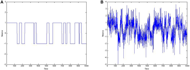
Figure 4. Binary big order return series before (A) and after (B) it has been corrupted by noise.

Our goal is to use SSR to mitigate the effect of the noise corruption and help us extract the big order signal. We measure the noise filtering success of SSR by the percentage increase in correlation coefficient. That is, we compute $\frac{corr(x^{*}(t),S(t))-corr(x(t),S(t))}{corr(x(t),S(t))}$. Following are results using N = {1, 10, 100, 1000, 10, 000} threshold units.

Figure 5 shows that SSR was pretty successful, topping out at a correlation coefficient increase of almost 5% when N = 10,000. We can observe that as the number of units increase, there is an increase in the peak of information gain. While the increase in the peak between plots corresponding to N = 100, 1000, and 10,000 is very minor, we can observe that as the number of threshold units increase, the data are more stable and the decline from the peak is more gradual.

FIGURE 5

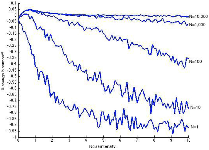
Figure 5. Post-SSR increase in correlation coefficient using N = {1, 10, 100, 1000, 10, 000} threshold units, over 1000 time units.

It is also important to note the tradeoff between the length of the signal used and amount of threshold units used. Reproducing the signal in Figure 4A nine times, so that the new signal has length 10,000, we compare the results to a close-up of the result for N = 10,000 in Figure 5 (close-up is shown in see Figure 6). We observe that the plot (Figure 7) is much less volatile using a longer signal.

FIGURE 6

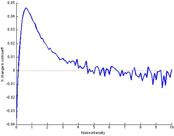
Figure 6. Close-up of post-SSR increase in correlation coefficient using N = 10,000 threshold units, over 1000 time units.

FIGURE 7

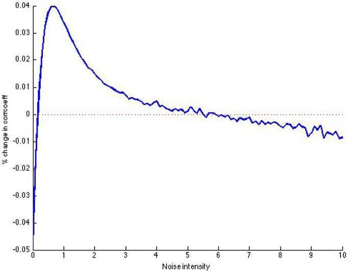
Figure 7. Post-SSR increase in correlation coefficient using 10,000 threshold units, over 10,000 time units.

2.2. SSR on Prices

As an alternative to attempting to yield a clearer return series, we try to yield a clearer price signal. Again, let's assume that we are either in a stream of big buy orders or big sell orders, each order affecting the price signal with an amount having the same magnitude (either 0.005 or –0.005). Let us suppose this signal is corrupted by Gaussian distributed noise [N(0, 1)] from small scale traders (Figure 8).

FIGURE 8

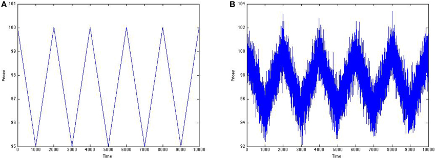
Figure 8. (A) Prices. (B) Prices after noise from small scale traders.

As can be seen in Figure 9, there is some information gained about the signal after SSR. Specifically, there is a noise induced maximum in increase of correlation coefficient of about 1%. The structure created in the price model is more complex than that of the return signal in Figure 4A, explaining the worse results.

FIGURE 9

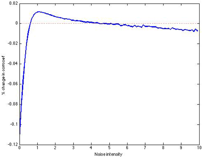
Figure 9. Post-SSR increase in correlation coefficient using 10,000 threshold units, over 10,000 time units.

2.3. Which Method?

In this paper we will discuss scenarios in which SSR on returns is favored over SSR on prices, and vice versa. First, it is important to note that the preferred method is dependent upon the level of noise of small scale traders. Consider the signal in Figures 8A,B. Here we assume that the corrupting noise is sampled from a standard normal distribution—this is intense relative to the signal. McDonnell et al. show that a maximum in mutual information must occur at a noise intensity of at most unity ($\frac{{\sigma }_n}{{\sigma }_x}\le 1$). Additionally, they qualitatively show that as N increases, the added noise intensity at which a maximum in mutual information occurs increases [22] (pp. 90–91). As our approach is different than Stocks', this is not necessarily true for our model. When σ_n = σ_x, the correlation coefficient between the price signal and the noisy price signal is 0.8212, and the correlation coefficient between the price signal and the output of SSR is 0.8315. Now, if we take the log returns of the pure signal, and of the noise-corrupted signal, we have the signals in Figure 10.

FIGURE 10

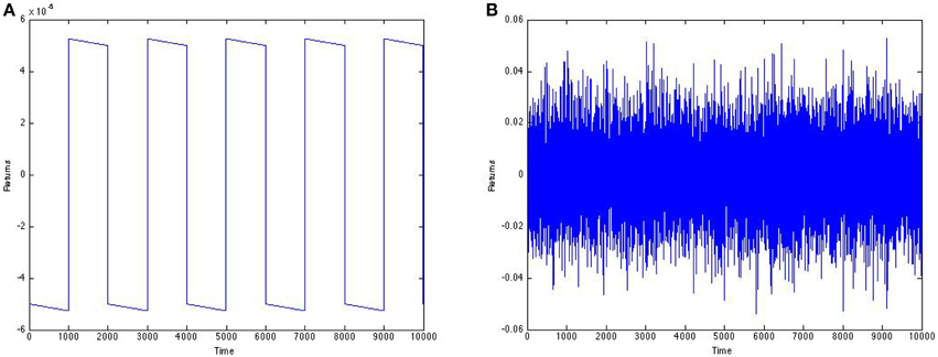
Figure 10. Return signal corresponding to the price signal in Figure 8A before and after noise. (A) Before noise. (B) After noise.

After computing log returns, the signal we wish to detect becomes roughly 1000 times smaller than the magnitude of the noisy signal. Extracting this signal seems futile. At an added noise intensity of unity, the correlation coefficient between the return signal and the noisy return signal is 0.0039 and the correlation coefficient between the return signal and the output of SSR is 0.0031—very low numbers compared to the analysis on the price signal.

Now, let us suppose the corrupting noise intensity is much smaller. For example, suppose the noise is sampled from a N(0, 0.003²) distribution.

With the views provided, it is difficult to distinguish between the signals in Figures 11A,B as the noise intensity corrupting the signal is very low. The correlation coefficient between the price signal and the noisy price signal is one. Clearly applying SSR to this signal will not improve the clarity of the signal. Adding noise to a clear signal is futile as it can only yield a distorted signal. However, these relatively small disturbances in the price signal can manifest into highly volatile log returns as seen in Figure 12B. In this situation, we are better served to use SSR on the returns, attempting to extract the signal in Figure 12A from the noisy signal in Figure 12B. As can be seen in Figure 13, the gain in correlation coefficient tops out at a very significant amount of about 6%. At an added noise intensity of 0.5, the correlation coefficient between the noise-corrupted return signal and the pure return signal is 0.7644, while the correlation coefficient between the output of SSR and the pure return signal is 0.8114.

FIGURE 11

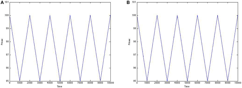
Figure 11. Prices before and after N(0, 0.003²) noise from small scale traders. (A) Before noise. (B) After noise.

FIGURE 12

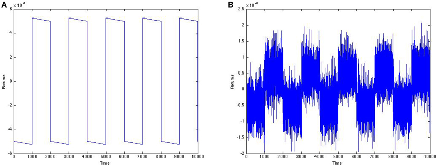
Figure 12. (A) Returns corresponding to the price signal in Figure 11A. (B) Returns corresponding to the price signal in Figure 11B.

FIGURE 13

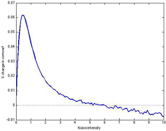
Figure 13. Increase in correlation coefficient as a function of added noise intensity to signal in Figure 12B (using 10,000 units).

Now we consider a signal that is a bit more realistic as it pertains to our financial application. We suppose broken down big orders, each of the same magnitude, are executed every 25 time units (Figure 14A), resulting in either an increase or decrease in price every 25 time units (of course this part is not too realistic). We first use heavy noise (Figure 14B).

FIGURE 14

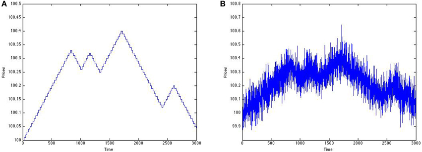
Figure 14. Prices before and after noise from small scale traders. (A) Before noise. (B) After noise.

The sign of each order in the signal in Figure 14A was determined by a Markov chain, with probability of 0.95 of staying within a state. Again, we achieve a gain in information after SSR (Figure 15).

FIGURE 15

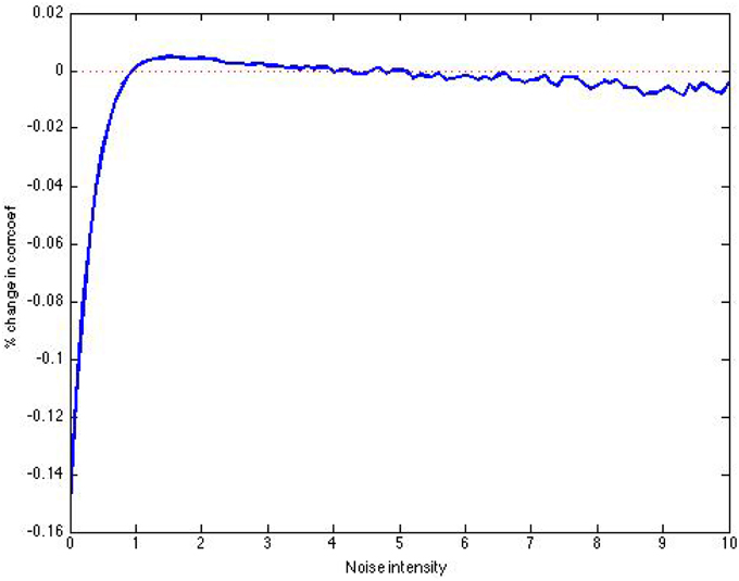
Figure 15. Post-SSR increase in correlation coefficient using 10,000 threshold units, over 3000 time units.

Next we lower the corrupting noise enough so that the correlation coefficient between a noisy price signal and the clear price signal is nearly 1, and the correlation coefficient between the corresponding noisy return signal and clear return signal is relatively high (say, between 0.7 and 0.9; see Figure 16).

FIGURE 16

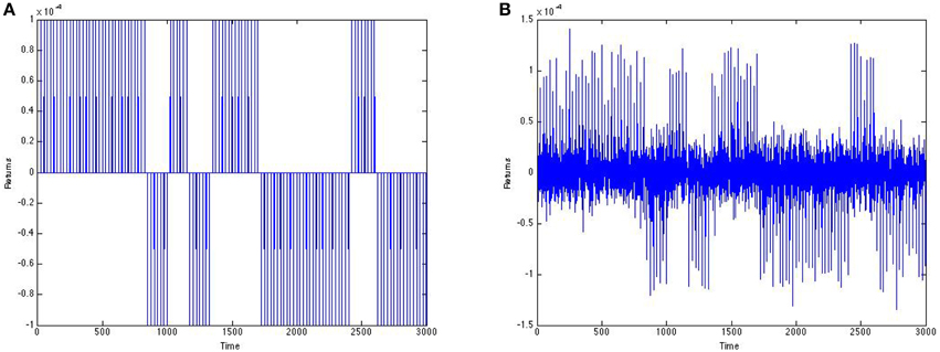
Figure 16. Returns before and after noise from small scale traders. (A) Before noise. (B) After noise.

Using increase in correlation coefficient as a measure of information gain, we in fact achieve none (see Figure 17). Another interesting point is that the closest we are to achieving information gain occurs at an added noise intensity of around 10, as opposed to an amount less than unity. We also have examples in which there is indeed information gain, and the peak occurs at a noise intensity greater than unity.

FIGURE 17

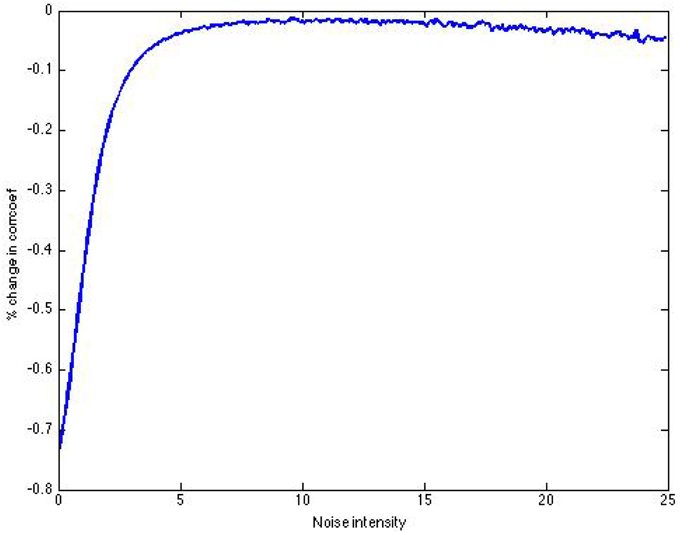
Figure 17. Post-SSR increase in correlation coefficient using 10,000 threshold units, over 3000 time units.

2.4. Preprocessing for HMM

A Hidden Markov Model (HMM) is a Markov Process where the states of the model are unknown (hidden). Based on the output of the model, it is possible to deduce information about the states, such as the probability of being in a state. We use a two state HMM in an attempt to capture high and low levels of returns.

2.4.1. Approach

In our simulations, we always constructed our noisy signal to be x(t) = S(t) + ξ(t) where S(t) is the clear signal we wish to detect and ξ(t) is noise. Therefore, we were able to measure the coherence between S(t) and the output of SSR. Of course with real data, we are only given x(t), and we hope to extract a good representation of S(t). The output of SSR should allow us to more clearly detect whether we are in the midst of a stream of big buy orders, or a stream of big sell orders. Thus, if we define two states to represent a stream of buy orders or a stream of sell orders, applying SSR to real data should provide a greater separation between these two states.

Here, we will present results of SSR using 15,000 threshold units applied to 10,000 min worth of AAPL data. We desired minute–minute data and chose AAPL arbitrarily. This data was taken from February 15, 2013 to March 25, 2013. Note that there exist 1000 min in between any two consecutive time stamps in the following figures. We will compare the ability of a HMM to detect states without SSR with the ability to do so after preprocessing with SSR. We hope to achieve a better separation of states in the HMM after preprocessing with SSR.

2.4.2. Approach #1

One approach is to apply SSR to prices, then feed the log returns of the output of SSR to a HMM. We should achieve good results if the noise corrupting the price signal is relatively high. In Figure 18A we plot AAPL prices and in Figure 18B we plot the output of SSR as applied to AAPL prices.

FIGURE 18

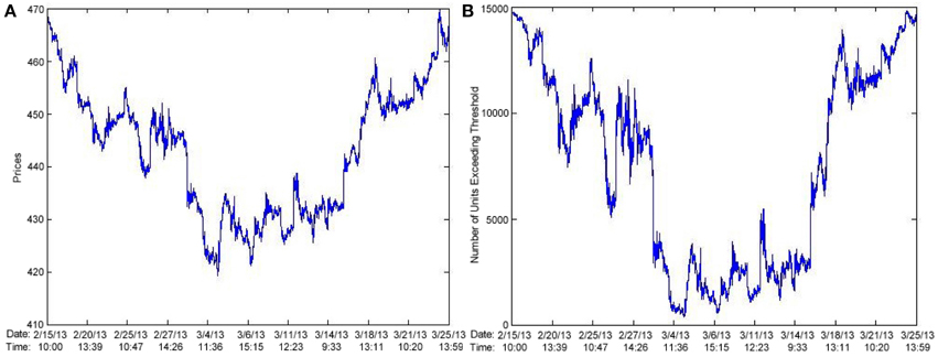
Figure 18. (A) AAPL prices. (B) Output of SSR applied to AAPL prices.

First, we fit a two-state fixed transition HMM to the unaltered AAPL returns and achieve the following results:

Transition matrix: $\left[\begin{array}{cc}0.9805& 0.0195\\ 0.0711& 0.9289\end{array}\right]$

Expected duration spent in regime #1: 51.40 min

Expected duration spent in regime #2: 14.07 min

Figure 19 shows the state probabilities over time.

FIGURE 19

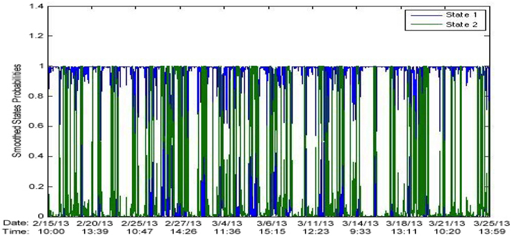
Figure 19. State probabilities over time.

We then preprocess our data with SSR at a noise intensity of unity. Then we feed the log returns of the output to a HMM. Following are the results:

Transition matrix: $\left[\begin{array}{cc}0.9893& 0.0107\\ 0.0116& 0.9884\end{array}\right]$

Expected duration spent in regime #1: 93.36 min

Expected duration spent in regime #2: 85.89 min

Figure 20 shows the state probabilities over time.

FIGURE 20

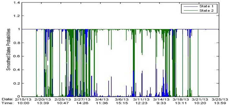
Figure 20. State probabilities over time with noise intensity of unity.

The results using a noise intensity of 1 were very exciting. It seemed like SSR really helped define/separate two regimes. Let us again consider the signal in Figures 8A,B.

Below are the results of fitting a HMM to the log returns of the noise-corrupted price signal in Figure 8B:

Transition matrix: $\left[\begin{array}{cc}0.8088& 0.1912\\ 0.1055& 0.8945\end{array}\right]$

Expected duration spent in regime #1: 5.23 min

Expected duration spent in regime #2: 9.48 min

Figure 21 shows the state probabilities over time.

FIGURE 21

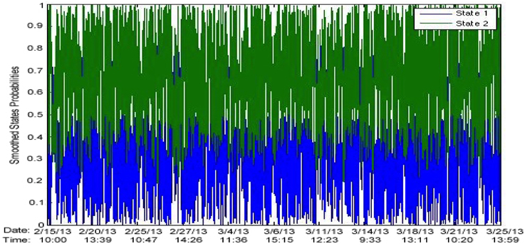
Figure 21. HMM on log returns of noise-corrupted signal in Figure 8B. State probabilities over time.

Recall that for the signal in Figures 8A,B, a near maximum in correlation coefficient increase occurred at noise intensity 1. Following are the results of fitting a HMM to the log returns of the output of SSR applied to the signal in Figure 8B, using a noise intensity of 1.

Transition matrix: $\left[\begin{array}{cc}0.9593& 0.0407\\ 0.0323& 0.9677\end{array}\right]$

Expected duration spent in regime #1: 24.58 min

Expected duration spent in regime #2: 30.94 min

Figure 22 shows the state probabilities over time.

FIGURE 22

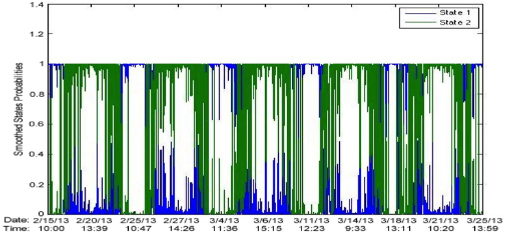
Figure 22. HMM on log returns of output of SSR on noise-corrupted signal in Figure 8B. State probabilities over time with noise intensity of unity.

These results again seem awfully promising. It seems like there is clearly a better separation of states after SSR. The issue is the location in which the state switching occurs. We would expect a state switch to occur at time multiples of 1000. This is not the case—instead, state switches occur at time points x + 500 where x is a non-negative multiple of 1000. Figure 23 is the plot of the log returns of the output of SSR.

FIGURE 23

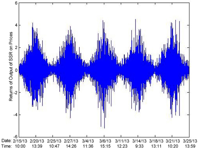
Figure 23. Plot of log returns of output of SSR applied to the noise-corrupted signal in Figure 8B.

In Figure 23 we observe high volatility corresponding to low values in the price signal, and low volatility for high values in the price signal. Going back to the results on AAPL stock; following (Figure 24) are plots of the price signal, and of the log returns of the output of SSR.

FIGURE 24

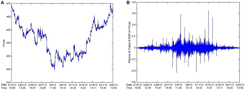
Figure 24. (A) AAPL prices. (B) Log returns of output of SSR on AAPL prices.

Again, we observe the same phenomenon. Suppose X(t) is the number of units that have exceeded the threshold at time t. Real data prices won't vary much between time t and time t + 1 (suppose we are using minute to minute data), but due to the stochastic nature of our results, |X(t + 1) − X(t)| could be large, and cause higher volatility in returns in periods of low price.

2.4.3. Approach #2

Another reasonable approach is to apply SSR to the returns and fit the results to a HMM. Figure 25A shows a plot of AAPL log returns and Figure 25B shows a plot of the output of SSR as applied to the AAPL log returns.

FIGURE 25

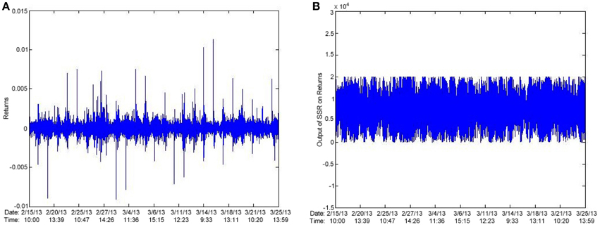
Figure 25. (A) AAPL returns. (B) Output of SSR applied to AAPL returns.

We preprocess AAPL returns with SSR at a noise intensity of unity. Following are the results:

Transition matrix: $\left[\begin{array}{cc}0.9923& 0.0077\\ 0.0068& 0.9932\end{array}\right]$

Expected duration spent in regime #1: 129.89 min

Expected duration spent in regime #2: 147.59 min

Figure 26 shows the state probabilities over time.

FIGURE 26

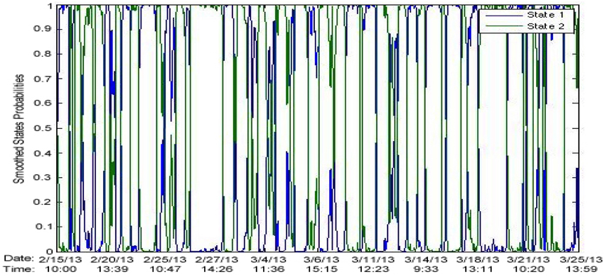
Figure 26. State probabilities over time with noise intensity of unity.

We observe that the two regimes are far more separated after preprocessing with SSR. There are certain data sets for which the results after SSR show no state switching. It appears that after SSR, a HMM becomes more susceptible to becoming stuck in a certain state. Using a three state HMM seems to fix this issue, however we leave elaboration for future work.

3. Discussion and Conclusion

The effect of stochastic resonance is often characterized as a rapid increase in information gain as a function of noise intensity. This is followed by a gradual decline from the peak [18]. Our many simulations clearly exhibit parallel findings, improving as the number of threshold units increase. This provides validity to our noise filtering application of SSR. Empirically, the noise filtering seems to be most effective when there is low variability in the underlying signal S(t) between consecutive time points. The extent of applicability of our model to financial markets remains to be determined. We plan to refine our results of fitting a HMM to the output of SSR applied to log returns and see if we can turn a profit with the knowledge of a potentially clearer signal.

Another subject for future work is threshold tuning. Stocks shows that the effect of SSR is maximized when all thresholds are set to the signal mean. Our application of SSR is different than his, and as such, it is worthwhile to investigate potential improvements from threshold tuning.

We have shown that fitting a HMM to the log returns of the output of SSR on prices is not a reasonable approach. SSR on prices can provide a clearer signal, so this methodology will be explored further. If the application of SSR to real data can really filter noise, we can use the results as an input to essentially any method. This leaves many doors wide open.

Conflict of Interest Statement

The authors declare that the research was conducted in the absence of any commercial or financial relationships that could be construed as a potential conflict of interest.

Acknowledgments

We would like to thank Yu Mu for his helpful suggestions and for providing input data.

References

1. Collins JJ, Chow CC, Imhoff TT. Aperiodic stochastic resonance in excitable systems. Phys Rev E (1995) 52:R3321–4. doi: 10.1103/PhysRevE.52.R3321

PubMed Abstract | CrossRef Full Text | Google Scholar

2. Benzi R, Sutera A, Vulpiani A. The mechanism of stochastic resonance. J Phys A Math Gen. (1981) 14:L453. doi: 10.1088/0305-4470

PubMed Abstract | CrossRef Full Text | Google Scholar

3. Nicolis C. Solar variability and stochastic effects on climate. Solar Phys. (1981) 74:473–8. doi: 10.1007/BF00154530

CrossRef Full Text | Google Scholar

4. Nicolis C. Stochastic aspects of climatic transitions response to a periodic forcing. Tellus (1982) 34:1–9. doi: 10.1111/j.2153-3490.1982.tb01786.x

CrossRef Full Text | Google Scholar

5. Nicolis C, Nicolis G. Stochastic aspects of climatic transitions Additive fluctuations. Tellus (1981) 33:225–34. doi: 10.1111/j.2153-3490.1981.tb01746.x

CrossRef Full Text | Google Scholar

6. Benzi R, Parisi G, Sutera A, Vulpiani A. A theory of stochastic resonance in climatic change. SIAM J Appl Math. (1983) 43:565–78. doi: 10.1137/0143037

CrossRef Full Text | Google Scholar

7. McNamara B, Wiesenfeld K, Roy R. Observation of stochastic resonance in a ring laser. Phys Rev Lett. (1988) 60:2626–9. doi: 10.1103/PhysRevLett.60.2626

PubMed Abstract | CrossRef Full Text | Google Scholar

8. Gammaitoni L, Hänggi P, Jung P, Marchesoni F. Stochastic resonance. Rev Mod Phys. (1998) 70:223–87. doi: 10.1103/RevModPhys.70.223

PubMed Abstract | CrossRef Full Text | Google Scholar

9. Collins JJ, Chow CC, Imhoff TT. Stochastic resonance without tuning. Nature (1995) 376:236–8. doi: 10.1038/376236a0

PubMed Abstract | CrossRef Full Text | Google Scholar

10. Heneghan C, Chow CC, Collins JJ, Imhoff TT, Lowen SB, Teich MC. Information measures quantifying aperiodic stochastic resonance. Phys Rev E (1996) 54:R2228–31. doi: 10.1103/PhysRevE.54.R2228

PubMed Abstract | CrossRef Full Text | Google Scholar

11. Longtin A. Stochastic resonance in neuron models. J Stat Phys. (1993) 70:309–27. doi: 10.1007/BF01053970

CrossRef Full Text | Google Scholar

12. Bulsara A, Jacobs EW, Zhou T, Moss F, Kiss L. Stochastic resonance in a single neuron model: theory and analog simulation. J Theor Biol. (1991) 152:531–55. doi: 10.1016/S0022-5193(05)80396-0

PubMed Abstract | CrossRef Full Text | Google Scholar

13. Douglass JK, Wilkens L, Pantazelou E, Moss F. Noise enhancement of information transfer in crayfish mechanoreceptors by stochastic resonance. Nature (1993) 365:337–340. doi: 10.1038/365337a0

PubMed Abstract | CrossRef Full Text | Google Scholar

14. Stocks N, Mannella R. Suprathreshold stochastic resonance in a neuronal network model: a possible strategy for sensory coding. In: Kasabov N, editor. Future Directions for Intelligent Systems and Information Sciences. Vol. 45 of Studies in Fuzziness and Soft Computing. Heidelberg: Physica-Verlag (2000). pp. 236–47.

Google Scholar

15. Stocks NG, Mannella R. Generic noise-enhanced coding in neuronal arrays. Phys Rev E (2001) 64:030902. doi: 10.1103/PhysRevE.64.030902

PubMed Abstract | CrossRef Full Text | Google Scholar

16. Longtin A, Bulsara A, Moss F. Time-interval sequences in bistable systems and the noise-induced transmission of information by sensory neurons. Phys Rev Lett. (1991) 67:656–9. doi: 10.1103/PhysRevLett.67.656

PubMed Abstract | CrossRef Full Text | Google Scholar

17. Longtin A, Bulsara A, Pierson D, Moss F. Bistability and the dynamics of periodically forced sensory neurons. Biol Cybern. (1994) 70:569–78. doi: 10.1007/BF00198810

PubMed Abstract | CrossRef Full Text | Google Scholar

18. Wiesenfeld K, Moss F. Stochastic resonance and the benefits of noise: from ice ages to crayfish and SQUIDs. Nature (1995) 373:33–6. doi: 10.1038/373033a0

PubMed Abstract | CrossRef Full Text | Google Scholar

19. Bulsara AR, Gammaitoni L. Tuning in to noise. Phys Today (1996) 49:39–47. doi: 10.1063/1.881491

CrossRef Full Text | Google Scholar

20. Gingl Z, Kiss LB, Moss F. Non-dynamical stochastic resonance: theory and experiments with white and arbitrarily coloured noise. Europhys Lett. (1995) 29:191. doi: 10.1209/0295-5075/29/3/001

CrossRef Full Text | Google Scholar

21. Stocks NG. Suprathreshold stochastic resonance in multilevel threshold systems. Phys Rev Lett. (2000) 84:2310–3. doi: 10.1103/PhysRevLett.84.2310

PubMed Abstract | CrossRef Full Text | Google Scholar

22. McDonnell MD, Stocks NG, Pearce CEM, Abbott D. Stochastic Resonance: From Suprathreshold Stochastic Resonance to Stochastic Signal Quantization. Cambridge, MA; New York, NY; Melbourne; Madrid; Cape Town; Singapore; Sao Paulo; Delhi: Cambridge University Press (2008).

Google Scholar

23. Stocks NG. Information transmission in parallel threshold arrays: suprathreshold stochastic resonance. Phys Rev E (2001) 63:041114. doi: 10.1103/PhysRevE.63.041114

PubMed Abstract | CrossRef Full Text | Google Scholar

24. Stocks NG. Suprathreshold stochastic resonance: an exact result for uniformly distributed signal and noise. Phys Lett A (2001) 279:308–12. doi: 10.1016/S0375-9601(00)00830-6

CrossRef Full Text | Google Scholar

25. McDonnell MD, Abbott D, Pearce CEM. An analysis of noise enhanced information transmission in an array of comparators. Microelectron J. (2002) 33:1079–89. doi: 10.1016/S0026-2692(02)00113-1

CrossRef Full Text | Google Scholar

26. Stocks NG, Allingham D, Morse RP. The application of suprathreshold stochastic resonance to cochlear implant coding. Fluctuat Noise Lett. (2002) 02:L169–81. doi: 10.1142/S0219477502000774

CrossRef Full Text | Google Scholar

27. McDonnell MD, Stocks NG, Pearce CEM, Abbott D. Optimal information transmission in nonlinear arrays through suprathreshold stochastic resonance. Phys Lett A (2006) 352:183–9.

Google Scholar

28. McDonnell MD, Abbott D. Signal reconstruction via noise through a system of parallel threshold nonlinearities. In: IEEE International Conference on Acoustics, Speech, and Signal Processing 2004 (ICASSP ′04), Vol. 2, Proceedings (2004). Montreal. pp. ii–809–12. doi: 10.1016/j.physleta.2005.11.068

CrossRef Full Text | Google Scholar

29. McDonnell MD, Stocks NG, Pearce CEM, Abbott D. Analog-to-digital Conversion using Suprathreshold Stochastic Resonance (2005), Sydney: SPIE International Symposium on Smart Structures, Devices, and Systems II.

Google Scholar

30. Lillo F, Farmer JD. The long memory of the efficient market. Stud. Nonlin. Dyn. Econ. (2004) 8:1–35. doi: 10.2202/1558-3708.1226

CrossRef Full Text | Google Scholar