The role of incompleteness in commodity futures markets

1. Introduction

A convenience yield is often used to describe the value to hold commodities as is explained in e.g., [1]. For example, natural gas is stored as a preemptive strategic action for power companies to keep steady power generation from gas-fired power plants in response to electricity demand variation. It implies that the storage of natural gas produces any positive value for the generator, which is represented as a convenience yield. More importantly, a convenience yield is able to represent the linkage between commodity spot and futures prices on commodity futures curves because it is also used to explain upward and downward sloping commodity futures curves referred to as contango and backwardation, respectively. On the other hand, asset pricing theory offers a concept of a stochastic discount factor to determine financial instrument prices including futures prices written on commodity spot prices. The relationship between commodity spot and futures prices is characterized by two representations: a convenience yield and stochastic discount factor. Putting two concepts together, a convenience yield may play an alternative role of a stochastic discount factor. This paper highlights the relationship between a convenience yield and stochastic discount factor and offers a commodity pricing representation based on the convenience yield.

A risk neutral valuation often used in financial markets is applied to commodity derivative pricing as in e.g., [2–8], among others. Recently, Trolle and Schwartz [9] developed a very sophisticated commodity price model using the HJM type forward cost of carry with stochastic volatility under the assumptions of a risk neutral measure not only for commodity spot prices but also for the cost of carry and unspanned volatility. However, it is generally difficult to price a commodity product such as commodity futures using the risk neutral valuation because commodity markets are incomplete due to their illiquidity. Hence, we have a further elaborate task to select a stochastic discount factor (SDF) in evaluating their value. A familiar tool to select a SDF is a utility-based approach where SDF, i.e., market price of risk, is assigned to the unspanned risk and the derivative prices are uniquely determined. For example, Davis [10] and Cao and Wei [11] characterize the prices of weather derivatives, which are generally categorized in commodity derivatives, using utility functions and optimal consumptions. This pricing approach may be tractable to determine the price. But, this method deeply has to depend on the selection of a utility function and optimal consumption. To avoid the imperfection of a utility-based approach and incorporate market incompleteness into commodity futures pricing, the good-deal bounds (GDB) is developed by Cochrane and Saa-Requejo [12]. The GDB pricing is new in the sense of introducing a restriction on the variance of a SDF: a certain upper SDF variance boundary is characterized by the maximum Sharpe ratio which must always exceed or be equal to Sharpe ratios of all assets in a market. As an example to price incomplete market assets, Kanamura and Ohashi [13] applied the GDB to weather derivatives. The GDB may be useful to price incomplete market assets in the sense that it does not rely on the utility function and optimal consumption like utility-based models. However, the method is still dissatisfactory because the maximum Sharpe ratio binding the SDF is unknown and thus must be given exogenously. A pricing scheme for commodities will be desirable if the Sharpe ratio, i.e., the restriction on a SDF, is given using commodity market data. We consider that two-way concept on intertemporal relationship between commodity spot and futures prices, i.e., a convenience yield can implicitly determine the SDF, will be useful to determine the Sharpe ratio. A convenience yield can offer the maximum Sharpe ratio, i.e., the market price of risk other than commodity spot market price of risk, which is used for commodity derivative pricing. This pricing scheme is referred to as “a convenience yield-based pricing.” This paper proposes a convenience yield-based pricing for commodity futures, which embeds the incompleteness of commodity futures markets in convenience yields.

Using the pricing method, we conduct empirical analyses of the prices of WTI crude oil, heating oil, and natural gas futures traded on the NYMEX to assess the incompleteness of energy futures markets. We show that the incompleteness of natural gas futures market is more highlighted than the incompleteness of WTI crude oil and heating oil futures markets. We apply the market price of risk embedded in the NYMEX data to pricing an Asian call option on WTI crude oil futures prices. Finally, we try to apply the market incompleteness analysis to the post-crisis periods after 2009.

This paper is organized as follows. Section 2 proposes a convenience yield-based pricing for commodity futures. Section 3 conducts empirical studies to examine the incompleteness of energy futures markets. Section 4 applies the empirical results to pricing an Asian call option on WTI crude oil futures prices. Section 5 tries to apply the market incompleteness analysis to the post-crisis periods after 2009. Section 6 concludes and offers a future direction of the study.

2. The Convenience Yield-based Pricing for Commodity Futures

Gibson and Schwartz [14] introduce a two-factor model for commodity spot prices, which represents a well-known price model in commodity markets. We start with the basic spot price model to obtain commodity futures prices. Commodity spot prices and convenience yields follow

$\begin{array}{rc}\frac{d{S}_t}{S_t}=(\mu -{\delta }_t)dt+{\sigma }_{1}d{w}_t,& (1)\end{array}$

$\begin{array}{rc}d{\delta }_t=\kappa (\alpha -{\delta }_t)dt+{\sigma }_{2}d{u}_t,& (2)\end{array}$

where E_t[dw_tdu_t] = ρdt. In Gibson and Schwartz [14], a convenience yield is treated as an important factor characterizing the relationship between commodity spot and futures prices.

Then we address the modeling of commodity futures prices. While [3] introduced a risk neutral measure to price commodity futures, the ambiguity may remain in the existence of such a probability measure. More importantly, the risk-neutral pricing, which is common in pricing of other derivatives, is not so appropriate to commodity futures markets because of the incompleteness nature of the commodity markets. Hence, we chose more comprehensive representation of the futures prices by using a stochastic discount factor (SDF). The futures prices $F_t^T$ at time t with maturity T are in general represented as follows:

$\begin{array}{cc}{F}_t^T=E_t\left[\frac{\frac{{\Lambda }_T}{{\Lambda }_t}{S}_T}{E_t\left[\frac{{\Lambda }_T}{{\Lambda }_t}\right]}\right],& \left(3\right)\end{array}$

where the SDF is denoted by Λ_t at time t and an interest rate is assumed to be constant (see e.g., [15, 16]).

To obtain commodity futures prices, we try to characterize the SDF in Equation (3). As is well known, commodity markets may demonstrate incompleteness because of the illiquidity. Following Cochrane and Saa-Requejo [12] which can generally express market incompleteness, we assume

$\begin{array}{rc}\frac{d{\Lambda }_t}{{\Lambda }_t}=-rdt-\varphi d{w}_t-\nu d{z}_t,& (4)\end{array}$

where ν demonstrates market incompleteness in the sense of the unspanned part by commodity spot markets. The point is that the market risk is composed of two risks from commodity spot market and its orthogonal part. Note that $\nu =\sqrt{A^2-{\varphi }^2}$ where A represents the Sharpe ratio exogenously given in Cochrane and Saa-Requejo [12].

Let us consider how the incompleteness, i.e., the orthogonal part to the commodity spot price risk, is described. The untraded convenience yield explains upward and downward sloping commodity futures curves, i.e., contango and backwardation, respectively, which includes illiquid delivery month commodity futures. Since a convenience yield is useful to connect commodity spot prices with the futures prices as is illustrated by two different points on commodity futures curves, convenience yields may be a key to represent incompleteness of commodity markets. In contrast, asset pricing theory offers a concept of a SDF to characterize futures prices written on commodity spot prices. Putting two ideas together, a convenience yield can play an alternative role of a SDF. We assume that the fluctuation due to convenience yield (du_t) is spanned by both of complete and incomplete parts (dw_t and dz_t, respectively):

$\begin{array}{rc}d{u}_t=\rho d{w}_t+\sqrt{1-{\rho }^2}d{z}_t& (5)\end{array}$

where ρ is constant¹. By using Ito's lemma to Equation (1), we obtain

$\begin{array}{rc}{S}_T=S_t{e}^{(\mu -\alpha -\frac{1}{2}{\sigma }_1^2)(T-t)+\frac{1}{\kappa }(1-e^{-\kappa (T-t)})({\delta }_t-\alpha )+{\displaystyle {\int }_t^T({\sigma }_1+\frac{{\sigma }_2\rho }{\kappa }(}1-e^{-\kappa (T-s)}))d{w}_s+{\displaystyle {\int }_t^T(\frac{{\sigma }_2\sqrt{1-{\rho }^2}}{\kappa }(}1-e^{-\kappa (T-s)}))d{z}_s}.& (6)\end{array}$

Again by using Ito's lemma to Equation (4), we obtain

$\begin{array}{rc}\frac{{\Lambda }_T}{{\Lambda }_t}=e^{-(r+\frac{1}{2}{\varphi }^2+\frac{1}{2}{\nu }^2)(T-t)-{\displaystyle {\int }_t^T\varphi }d{w}_s-{\displaystyle {\int }_t^T\nu }d{z}_s}.& (7)\end{array}$

Injecting Equations (6) and (7) into Equation (3), we have commodity futures price as follows:

$\begin{array}{rc}{F}_t^T=S_t{e}^{\Upsilon (t,T)-\Omega (t,T){\delta }_t},& (8)\end{array}$

$\begin{array}{l}\Upsilon (t,T)=\left(r-\alpha +\frac{{\sigma }_2^2}{2{\kappa }^2}-\frac{{\sigma }_1{\sigma }_2\rho }{\kappa }+\varphi \frac{{\sigma }_2\rho }{\kappa }+\frac{\nu {\sigma }_2\sqrt{1-{\rho }^2}}{\kappa }\right)\\ (T-t)+\frac{{\sigma }_2^2}{4{\kappa }^3}(1-e^{-2\kappa (T-t)})+(\alpha \kappa +\rho {\sigma }_1{\sigma }_2-\frac{{\sigma }_2^2}{\kappa }\\ -\varphi {\sigma }_2\rho -\nu {\sigma }_2\sqrt{1-{\rho }^2})\frac{1-e^{-\kappa (T-t)}}{{\kappa }^2},& (9)\end{array}$

$\begin{array}{rc}\Omega (t,T)=\frac{1-e^{-\kappa (T-t)}}{\kappa }.& (10)\end{array}$

It is referred to as a convenience yield-based pricing for commodity futures (CY-based pricing) because convenience yields behave like a SDF to connect commodity spot prices with the futures prices. The point of this representation is in the inclusion of market incompleteness parameter ν into commodity spot-futures price relationship. A great advantage of the pricing is able to estimate the incomplete market price of risk ν directly from market data without an exogenous Sharpe ratio. We obtained a commodity futures pricing representation not using a risk neutral measure in complete market setting, but using an incompleteness parameter ν embedded in convenience yields.

If commodity futures are traded with high liquidity and all maturity date products are transacted in the market, i.e., T is not restricted as certain point of time, commodity futures price risk would be completely spanned in the market and ν might represent the market price of commodity futures risk unspanned by the spot price risk. However, the liquidity of commodity futures markets may be quite low in a certain delivery time, in particular longer maturity. In addition, the maturity date T is limited, say, 1-, 2-, 3- months, and so forth. ν includes the incomplete part neither spanned by existing commodity spot prices nor the futures prices and the incomplete part spanned by low liquidity commodity futures products. In this sense, we injected all the other market price of risk other than commodity spot markets, in particular commodity futures price risk both for high or low liquidity traded products and untraded delivery months or years products, into convenience yields. The CY-based pricing has an advantage to model all delivery commodity futures products irrelevant to the listed or unlisted delivery months as well as irrelevant to the liquidity. In addition, commodity futures markets provide the futures prices despite no trading volume. The information of ν implied from commodity futures markets will be beneficial to know how the overall maximum Sharpe ratio expands when non traded assets like newly developed derivatives instruments written on the same underlying commodities are introduced into the market. This is because it is expected that the risk premium for illiquid commodity futures products including no traded commodity futures is the same degree as the risk premium for newly traded derivative products within the same underlying commodity. The additional derivative market price of risk will be enveloped by ν. ν implied from commodity futures markets may be applicable to the other related derivative pricing. Then we examine the relationship between our pricing representation and existing models. Comparing our pricing representation to Bjerksund [2], the market price of convenience yield risk λ in Bjerksund [2] holds for

$\begin{array}{rc}\lambda =\varphi \rho +\nu \sqrt{1-{\rho }^2}.& (11)\end{array}$

Note that for Schwartz [3], the relation is changed into $\frac{\lambda }{{\sigma }_2}=\varphi \rho +\nu \sqrt{1-{\rho }^2}$. These relationships suggest that the market price of convenience yield risk is found to be split into two parts: a complete market price of risk and incomplete market price of risk, which are weighed using the correlation between commodity spot price returns and convenience yields. We can find that the market price of convenience yield risk denoted by λ includes untraded and unspanned risk of ν by connecting the SDF with convenience yields. In addition, the breakdown of the market price of risk can facilitate the treatment of the incompleteness not only for empirical analyses of commodity market incompleteness, but also for derivative pricing written on commodity futures prices. Our focus is to bring a new idea to the pricing representation by introducing an incomplete market price of risk embedded in convenience yields. In this sense, we offer the other interpretation of Bjerksund [2] and Schwartz [3] models not relying on a risk neutral measure.

3. Empirical Studies for Energy Futures Prices

3.1. Data

In this study, we use daily closing prices of WTI crude oil (WTI), heating oil (HO), and natural gas (NG) futures traded on the NYMEX. Each energy futures product includes six delivery months—from 1 to 6 months. The covered period of time is from April 3, 2000 to March 31, 2008. The data are obtained from the Bloomberg. Summary statistics for WTI, HO, and NG futures prices are provided in Tables 1–3, respectively. These tables indicate that WTI, HO, and NG have common skewness characteristics. The skewness of WTI, HO, and NG futures prices is positive, meaning that the distributions are skewed to the right.

TABLE 1

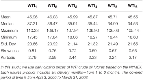
Table 1. Basic statistics of WTI crude oil futures prices.

TABLE 2

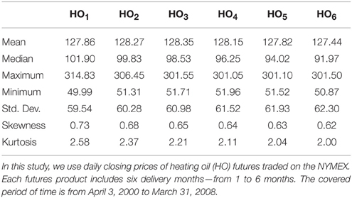
Table 2. Basic statistics of heating oil futures prices.

TABLE 3

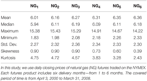
Table 3. Basic statistics of natural gas futures prices.

Then we examine the mean reversion of commodity futures price spreads. Here we define the price spreads by the differences of the logs of commodity futures prices: $S{P}_t^{ij}=log{F}_t^i-log{F}_t^j$ (i < j). By doing so, the influence of commodity spot prices is offset when commodity futures prices are expressed by the multiplication of the spot price and the exponential of convenience yield function as in Equation (9). In addition, $S{P}_t^{ij}$ may correspond to the level of convenience yields while the time dependent coefficient Ω(t, T) may exist. Hence, $S{P}_t^{ij}$ examination will detect the characteristics of convenience yields in the first order approximation. We estimate the model of commodity futures price spreads using

$\begin{array}{rc}S{P}_t^{ij}={\rho }_0+{\rho }_{1}S{P}_{t-1}^{ij}+{\eta }_t,& (12)\end{array}$

where i and j represent two different delivery months selected from 1- to 6-months (i < j), respectively. Table 4 reports the estimation results using 1- and 2-month WTI crude oil, heating oil, natural gas futures price spreads, respectively. According to the estimated ρ₁'s and the corresponding standard errors in the table, the price spreads demonstrate mean reversion. It implies that there exists another mean-reverting process in the futures price spreads other than the spot price process. Taking into account the price spread definition and constant Ω(t, T) because of generic energy futures products, i.e., approximately constant T − t, convenience yields for energy futures prices may correspond to a mean reverting process other than the spot price process, which supports the model structure using convenience yields.

TABLE 4

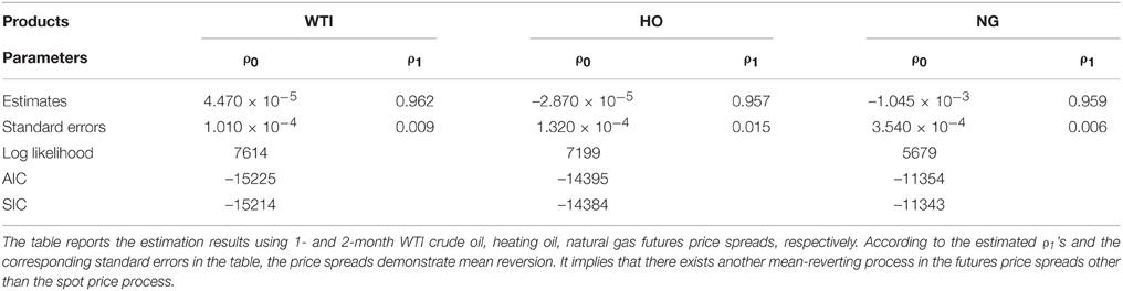
Table 4. Mean reversion of energy futures price spreads.

3.2. Parameter Estimation

We try to estimate the model parameters for CY-based pricing by using the Kalman filter in order to examine the incompleteness of energy futures markets. To simplify the calculation, we take log transformation of the spot price S_t into new variable x_t:

$\begin{array}{rc}d{x}_t=(\mu -\frac{1}{2}{\sigma }_1^2-{\delta }_t)dt+{\sigma }_{1}d{z}_t.& (13)\end{array}$

The Kalman filter consists of time and measurement update equations. On one hand, since x and δ in Equations (13) and (2), respectively are time updated, these equations represent linear time update equations in the Kalman filter system. We discretize the continuous-time model for x in Equation (13) into

$\begin{array}{rc}{x}_t=x_{t-1}-\Delta t{\delta }_t+\text{}(\mu -\frac{1}{2}{\sigma }_1^2)\Delta t\text{}+{\sigma }_1{ϵ}_t\equiv f_1(x_{t-1},{\delta }_{t-1},{ϵ}_t).& (14)\end{array}$

Similarly, the continuous-time model for δ in Equation (2) into the following:

$\begin{array}{rc}{\delta }_t=(1-\kappa \Delta t){\delta }_{t-1}+\kappa \alpha \Delta t+{\sigma }_2{\eta }_t\equiv f_2(x_{t-1},{\delta }_{t-1},{\eta }_t).& (15)\end{array}$

On the other hand, measurement update equation in the Kalman filter system is obtained from commodity futures-spot price relationship. We define the log of $F_t^T$ by new variable y_t ($y_t=\text{ln}{F}_t^T$), and discretize Equation (8) into the following:

$\begin{array}{rc}{y}_t=x_t-\Omega (t,T){\delta }_t+\Upsilon (t,T)+{\xi }_t\equiv h_1(x_t,{\delta }_t,{\xi }_t).& (16)\end{array}$

Following Welch and Bishop [18], the time and measurement update equations of the model are represented by

$\begin{array}{ll}\left(\begin{array}{c}\begin{array}{l}{x}_t\\ {\delta }_t\end{array}\end{array}\right)=\left(\begin{array}{c}\begin{array}{l}{\tilde{x}}_t\\ {\tilde{\delta }}_t\end{array}\end{array}\right)+A_t\left(\begin{array}{c}\begin{array}{l}{x}_{t-1}-{\widehat{x}}_{t-1}\\ {\delta }_{t-1}-{\widehat{\delta }}_{t-1}\end{array}\end{array}\right)+W_t\left(\begin{array}{c}\begin{array}{l}{ϵ}_t\\ {\eta }_t\end{array}\end{array}\right),\hfill & (17)\end{array}$

$\begin{array}{rc}{y}_t=h_1({\tilde{x}}_t,{\tilde{\delta }}_t,0)+B_t\left(\begin{array}{c}\begin{array}{l}{x}_t-{\tilde{x}}_t\\ {\delta }_t-{\tilde{\delta }}_t\end{array}\end{array}\right)+V_t{\xi }_t,& (18)\end{array}$

where ${\tilde{x}}_t=f_1({\widehat{x}}_{t-1},{\widehat{\delta }}_{t-1},0)$, ${\tilde{\delta }}_t=f_2({\widehat{x}}_{t-1},{\widehat{\delta }}_{t-1},0)$,
$\begin{array}{l}{A}_t=\left(\begin{array}{cc}1& -\Delta t\\ 0& 1-\kappa \Delta t\end{array}\right),W_t=\left(\begin{array}{cc}{\sigma }_1& 0\\ 0& {\sigma }_2\end{array}\right),B_t=\left(\begin{array}{cc}1& -\frac{1}{\kappa }(1-e^{-\kappa (T-t)})\end{array}\right),\\ V_t=1,V[{ϵ}_t,{\eta }_t]=Q_t=\left(\begin{array}{cc}\Delta t& \gamma \Delta t\\ \gamma \Delta t& \Delta t\end{array}\right)\end{array}$
, and V[ξ_t] = R_t = diag[m₁, m₂, m₃, m₄, m₅, m₆] (Diagonal matrix) where m_i ≥ 0 for i = 1 − 6.

Note that both of ϵ_t and η_t are the process noises, ξ_t is the measurement noise, and m₁ to m₆ are the volatilities of the measurement noises for the log prices of 1–6 months time to maturity futures products, respectively. Tables 5, 6 show the complete set of the Kalman filter equations which include the time and measurement update equations so as to calculate the a priori estimate the error covariance matrix (${\Phi }_t^{-}$) and the a posteriori estimate error covariance matrix (Φ_t), respectively.

TABLE 5

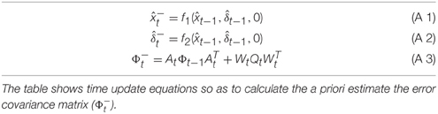
Table 5. Kalman filter time update equations.

TABLE 6

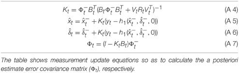
Table 6. Kalman filter measurement update equations.

Note that we define the a priori estimate error and the covariance by $e_t^{-}\equiv \left(\begin{array}{c}{x}_t-{\widehat{x}}_t^{-}\\ {\delta }_t-{\widehat{\delta }}_t^{-}\end{array}\right)$ and ${\Phi }_t^{-}\equiv E\left[e_t^{-}{e}_t^{-T}\right]$, and that we also define the a posteriori estimate error and the covariance by $e_t\equiv \left(\begin{array}{c}{x}_t-{\widehat{x}}_t\\ {\delta }_t-{\widehat{\delta }}_t\end{array}\right)$ and ${\Phi }_t\equiv E\left[e_t{e}_t^T\right]$ where K_t is the Kalman gain. Using the recursive updates of the time and measurement update equations as in Tables 5, 6, the measurement errors (ẽ_yt) and the covariance matrices (Σ_t) are given by

$\begin{array}{rc}{\tilde{e}}_{y_t}=y_t-h_1({\widehat{x}}_t^{-},{\widehat{\delta }}_t^{-},0),& (19)\end{array}$

$\begin{array}{rc}{\Sigma }_t=B_t{\Phi }_t^{-}{B}_t^T+V_t{R}_t{V}_t^T.& (20)\end{array}$

Using the measurement errors and the covariance matrices, the parameters (Θ) in Equations (1) and (2) are estimated by the maximum likelihood method

$\begin{array}{rc}\widehat{\Theta }=\text{arg}\underset{\Theta }{\min }{\displaystyle \sum _{t=1}^N\text{ln}}|{\Sigma }_t|+{\displaystyle \sum _{t=1}^N{\tilde{e}}_{y_t}}{\Sigma }_t^{-1}{\tilde{e}}_{y_t}^T,& (21)\end{array}$

where Θ = (μ, σ₁, κ, α, σ₂, ρ, ν, m₁, m₂, m₃, m₄, m₅, m₆). Note that a risk free rate r is set to 6%.

We estimated the parameters Θ for WTI crude oil, heating oil, and natural gas futures as reported in Tables 7–9, respectively. The parameters except m₃, m₄, and m₅ for WTI are statistically significant according to Table 7. Since ρ is estimated as 0.857 which is different from 1, it is shown that the fluctuation from the incompleteness is partly driven by the fluctuation from the convenience yield in Equation (5). In addition, the positive ρ is consistent with the view for a convenience yield as an embedded timing option to the commodity as discussed in Geman [1]. Then, according to Cochrane [19], negative ν generates the price upper boundary for the relevant derivative products. It implies that the market incompleteness due to the futures trading including illiquid delivery months may request the additional positive risk premium for WTI crude oil derivatives comparing to the spot market price of risk. While the futures market evolution increased the Sharpe ratio by negative ν in the orthogonal direction to dw_t, the absolute value regarding ν is relevant because the incompleteness due to the illiquidity can produce positive and negative risk premium². In this case, the incompleteness of WTI crude oil market is calculated as |ν| = 1.404 using the market data. Hence, we could directly obtain the incomplete market price of risk without using the exogenous Sharpe ratio. Then, we examine the results for heating oil. The parameters except α, m₂, m₃, and m₄ are statistically significant according to Table 8. Since ρ is statistically significant as 0.745, it is also shown that the fluctuation of the incompleteness partly stems from the fluctuation of the convenience yield in Equation (5). Additionally taking into account that it is smaller than the WTI correlation, the orthogonal fluctuation for the HO may contribute more to the convenience yield fluctuation than WTI in Equation (5). Since ν is statistically significant, the incompleteness of the heating oil market could be obtained using the market data. Finally examining the results for the natural gas in Table 9, the parameters except μ and α are statistically significant. In addition to the existence of incompleteness from the convenience yield, we also obtained the incomplete natural gas market price of risk using the market data.

TABLE 7

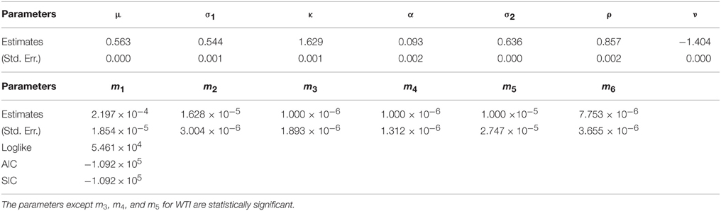
Table 7. Parameter estimation of WTI crude oil futures.

TABLE 8

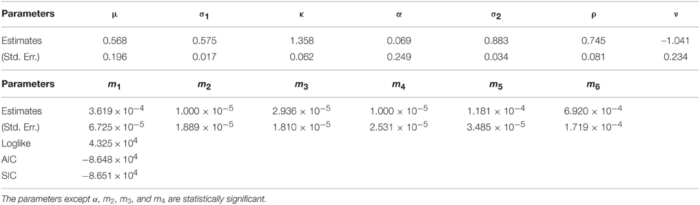
Table 8. Parameter estimation of heating oil futures.

TABLE 9

Table 9. Parameter estimation of natural gas futures.

Let us discuss the incompleteness of energy futures markets by comparing to the complete market price of risk. ϕ represents market price of risk for the complete market portion of commodity futures while ν demonstrates market price of risk for the incomplete market portion of commodity futures. The comparisons between ϕ and ν, not the absolute values, will explain how much the incompleteness of commodity futures markets affects the pricing of the commodity futures. The comparisons between ϕ and ν are reported in Table 10. Note that the completeness parameter ϕ is calculated as $\varphi =\frac{\mu -r}{{\sigma }_1}$ where we assume r = 0.06. “A” represents the Sharpe ratio defined as the square of the sum of two squared market prices of risks. For the WTI crude oil, the incomplete market price of risk (1.404) is a little greater than the complete market price of risk (0.924). It suggests that the WTI crude oil market should explicitly be spanned by both complete and incomplete markets. The Sharpe ratio is calculated as 1.681. It implies that the pricing of derivative instruments written on WTI crude oil prices just requires to introduce the Sharpe ratio of about twice (1.681) as large as the complete market price of risk (0.924) based on the GDB in Cochrane [19]. For heating oil, the Sharpe ratio takes a value of 1.365 with |ϕ| = 0.883 while the Sharpe ratio for the natural gas is obtained as 0.807 with |ϕ| = 0.302³. It is shown that the portion of the complete parts from WTI crude oil and heating oil in the whole Sharpe ratio is bigger than that from natural gas. This may be consistent with the fact that oil-related markets such as WTI crude oil and heating oil futures are more liquid than natural gas markets⁴.

TABLE 10

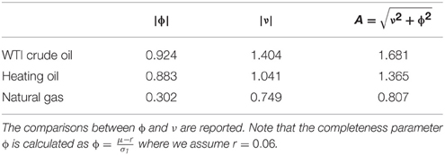
Table 10. Incompleteness of energy futures markets.

Since ν is larger than ϕ for all three products, it is found that unspanned risk by the spot prices asks for larger reward, i.e., higher Sharpe ratio, than spanned risk by the spot prices. It implies that unspanned part including commodity futures price risk may play an important role in the SDF in commodity futures markets. In addition, it may correspond to the origins of the development of commodity futures markets to reduce higher volatility in the spot prices. In particular, for natural gas which will be expected to have the highest volatility of the three, ν is around twice as large as ϕ, which is the biggest ν∕ϕ ratio of the three. It may be because volatility risk of natural gas prices may be more spanned by the unspanned part including the futures price risk than the other two commodities.

4. Application of CY-based Pricing to Energy Derivatives

4.1. Partial Differential Equation

The previous section derived the incomplete market price of risk (ν) from energy futures markets. ν will be useful to price newly introduced derivative products written on the same underlying asset because the illiquid futures products are taken as the same to newly introduced derivative in the sense that both these assets have no trading volume. Thus, ν may represent how the introduction of new products expands the whole market Sharpe ratio and may be applicable to the derivative pricing. We try to conduct the pricing of an Asian call option on energy futures prices using the good-deal bounds of Cochrane and Saa-Requejo [12]. The point is that ν is endogenously given by the parameters which have already estimated in Section 3, while ν is arbitrarily given in the good-deal bounds framework. In general, the GDB pricing is represented by

$\begin{array}{cc}{\underset{\_}{C}}_t=E_t{{\displaystyle \int }}_{s=t}^T\frac{{\underset{\_}{\Lambda }}_s}{{\underset{\_}{\Lambda }}_t}{x}_{s}ds+E_t\left(\frac{{\underset{\_}{\Lambda }}_T}{{\underset{\_}{\Lambda }}_t}{x}_T\right),& \left(22\right)\end{array}$

$\begin{array}{rc}\frac{d{\underset{\_}{\Lambda }}_t}{{\underset{\_}{\Lambda }}_t}=-rdt-\varphi d{w}_t\mp \nu d{z}_t,& (23)\end{array}$

where x_sds and x_T represent continuous dividends and a terminal payoff and ∓ represents lower and upper price boundaries, respectively. We for simplicity assume that the average i-month futures price from times 0 to T is given by

$\begin{array}{rc}I=\frac{1}{T}{\displaystyle {\int }_0^T{F}^i}(S,\delta ,t)dt.& (24)\end{array}$

Note that i is constant because we use generic energy futures prices and thus we neglect the superscript i below. We denote a price boundary by C(S, δ, I, t). We have

$\begin{array}{rc}\frac{d\underset{\_}{C}}{\underset{\_}{C}}={\mu }_{\underset{\_}{C}}dt+{\sigma }_{\underset{\_}{C}w}dw+{\sigma }_{\underset{\_}{C}z}dz.& (25)\end{array}$

The GDB pricing is transformed into

$\begin{array}{rc}{\mu }_{\underset{\_}{C}}-r+{\sigma }_{\underset{\_}{C}w}\mp {\sigma }_{\underset{\_}{C}z}\nu =0,& \left(26\right)\end{array}$

where ∓ represents lower and upper price boundaries, respectively. Note that x_s = 0.

By applying Ito's lemma to C(S, δ, I, t), we have

$\begin{array}{l}{\mu }_{\underset{\_}{C}}=\frac{1}{\underset{\_}{C}}\{\frac{\partial \underset{\_}{C}}{\partial t}+(\mu -\delta )S\frac{\partial \underset{\_}{C}}{\partial S}+\kappa (\alpha -\delta )\frac{\partial \underset{\_}{C}}{\partial \delta }+\frac{1}{2}{\sigma }_1^2{S}^2\frac{{\partial }^2\underset{\_}{C}}{\partial S^2}\hfill \\ +\frac{1}{2}{\sigma }_2^2\frac{{\partial }^2\underset{\_}{C}}{\partial {\delta }^2}+\rho {\sigma }_1{\sigma }_{2}S\frac{{\partial }^2\underset{\_}{C}}{\partial \delta \partial S}+\frac{1}{T}F\frac{\partial \underset{\_}{C}}{\partial I}\},\hfill \\ {\sigma }_{\underset{\_}{C}w}=\frac{1}{\underset{\_}{C}}\left\{\mu S\frac{\partial \underset{\_}{C}}{\partial S}+\rho {\sigma }_2\frac{\partial \underset{\_}{C}}{\partial \delta }\right\},\hfill \\ {\sigma }_{\underset{\_}{C}z}=\frac{1}{\underset{\_}{C}}\left\{{\sigma }_2\sqrt{1-{\rho }^2}\frac{\partial \underset{\_}{C}}{\partial \delta }\right\}.\hfill \end{array}$

The GDB upper and lower price boundaries of an Asian energy derivative are given as the solution of the following PDE by injecting μ_C, σ_Cw, and σ_Cz into Equation (26):

$\begin{array}{cc}\begin{array}{l}-r\underset{\_}{C}+\frac{\partial \underset{\_}{C}}{\partial t}+\frac{1}{2}{\sigma }_1^2{S}^2\frac{{\partial }^2\underset{\_}{C}}{\partial S^2}+\frac{1}{2}{\sigma }_2^2\frac{{\partial }^2\underset{\_}{C}}{\partial {\delta }^2}+\rho {\sigma }_1{\sigma }_{2}S\frac{{\partial }^2\underset{\_}{C}}{\partial \delta \partial S}+\frac{dI}{dt}\frac{\partial \underset{\_}{C}}{\partial I}\\ =(\delta -r)S\frac{\partial \underset{\_}{C}}{\partial S}+(\varphi \rho {\sigma }_2-\kappa (\alpha -\delta )\\ +k\nu {\sigma }_2\sqrt{1-{\rho }^2}\text{sgn}\left(\frac{\partial \underset{\_}{C}}{\partial \delta }\right))\frac{\partial \underset{\_}{C}}{\partial \delta },\end{array}& \left(27\right)\end{array}$

with the terminal payoff:

$\begin{array}{rc}\underset{\_}{C}(S,\delta ,I,T)=f(I_T),& (28)\end{array}$

where k = −1 and +1 generate the upper and lower price boundaries, respectively.

To obtain the GDB prices of the Asian call option, we set the payoff at the maturity to be f(I_T) = max(I_T − K, 0) and, following Ingersoll [20], $\frac{dI}{dt}$ to be

$\begin{array}{rc}dI=\frac{1}{\overline{T}}F(S,\delta ,t)dt.& (29)\end{array}$

4.2. Asian Call Option Price

We computed Asian call option prices written on 1-month WTI crude oil futures prices assuming that the strike price is 70 USD, the initial convenience yield is zero, and the interest rate is set to 6 %. The results are reported in Figure 1 and Table 11. Figure 1 suggests that both upper and lower risk premiums are small enough comparing with the level of the option prices because the three price curves are almost seen on the same line. It may be easily used for practitioners in the sense that the option price is obtained using very small price premiums. Then in order to examine the detailed risk premiums, the upper and lower risk premiums are calculated in Table 11. According to Table 11, the upper and lower risk premiums take the same value one another irrelevant to the initial futures prices. For example, the upper and lower premiums are calculated as 0.05 at the 80 USD initial WTI crude oil futures price. It may imply that both of seller and buyer of the option request the same risk premium to the WTI crude oil market incompleteness. Like these, we could show an example to calculate the risk premium based on the incompleteness of energy futures market implied from the CY-Based pricing we proposed.

FIGURE 1

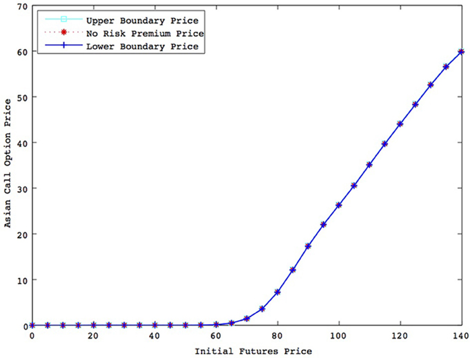
Figure 1. Asian call option prices (K = 70, δ = 0). The figure suggests that both upper and lower risk premiums are small enough comparing with the level of the option prices because the three price curves are almost seen on the same line.

TABLE 11

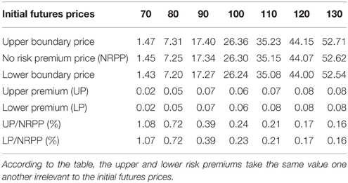
Table 11. Asian call option risk premium.

5. Post-crisis Analysis

One may think that it would be interesting to apply this market incompleteness analysis in Section 3 to the post-crisis periods after 2009. This section tries to conduct further empirical studies of the commodity futures prices using the data periods from January 2, 2009 to March 30, 2012. The results for the parameter estimations for the models of WTI crude oil, heating oil, and natural gas futures prices are reported in Tables 12–14.

TABLE 12

Table 12. Parameter estimation of WTI crude oil futures (post-crisis periods).

The parameters except m₃ and m₅ for WTI are statistically significant according to Table 12. Since ρ is estimated as 0.742 which is different from 1, it is shown that the fluctuation from the incompleteness is partly driven by the fluctuation from the convenience yield in Equation (5). In addition, the positive ρ is consistent with the view for a convenience yield as an embedded timing option to the commodity as discussed in Geman [1]. Then, according to Cochrane [19], negative ν generates the price upper boundary for the relevant derivative products. It implies that the market incompleteness due to the futures trading including illiquid delivery months may request the additional positive risk premium for WTI crude oil derivatives comparing to the spot market price of risk. While the futures market evolution increased the Sharpe ratio by negative ν in the orthogonal direction to dw_t, the absolute value regarding ν is relevant because the incompleteness due to the illiquidity can produce positive and negative risk premium. In this case, the incompleteness of WTI crude oil market is calculated as |ν| = 0.640 using the market data. It is found that the incomplete market price of risk in post-crisis periods is smaller comparing to the result in pre-crisis periods in Table 7 (|ν| = 1.404). Then, we examine the results for heating oil. The parameters except m₃ and m₅ are statistically significant according to Table 13. Since ρ is statistically significant as 0.692, it is also shown that the fluctuation of the incompleteness partly stems from the fluctuation of the convenience yield in Equation (5). Since ν is statistically significant, the incompleteness of the heating oil market could be obtained as |ν| = 0.518 using the market data. It is also demonstrated that the incomplete market price of risk in post-crisis periods is smaller comparing to the result in pre-crisis periods in Table 8 (|ν| = 1.041). Finally examining the results for the natural gas in Table 14, the parameters except μ, α, ν, and m₅ are statistically significant. Contrary to the result in pre-crisis periods in Table 9, we could not obtain the statistically significant incomplete natural gas market price of risk using the market data.

TABLE 13

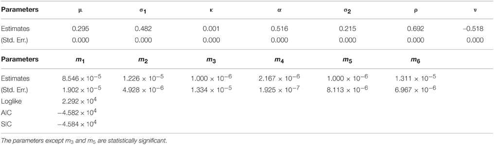
Table 13. Parameter estimation of heating oil futures (post-crisis periods).

TABLE 14

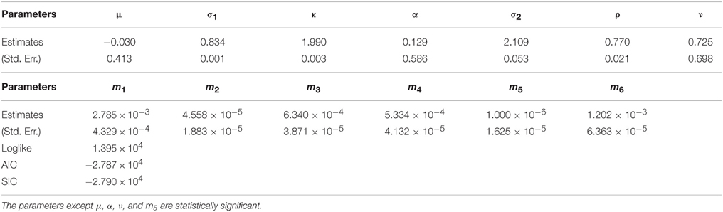
Table 14. Parameter estimation of natural gas futures (post-crisis periods).

In summary, comparing to the results for pre-crisis periods, the incomplete market prices of risk are obtained as smaller or negligible values in post-crisis periods. This may be interpreted as the shrink of the market incompleteness of commodity futures after 2008 financial crisis due to the increase of the market liquidity seen as the financialization of commodity markets⁵. In addition, the natural gas market price of risk is smaller than the other WTI crude oil and heating oil market prices of risk, which is different from the results for pre-crisis periods in Section 3. This may be explained by the increases of the liquidity in natural gas markets after 2008 financial turmoil because of the price drops through the US Shale gas revolution, which make the natural gas prices relatively cheap.

6. Conclusion

This paper has proposed a convenience yield-based pricing for commodity futures, which embeds the incompleteness of commodity futures markets in convenience yields. The characteristics of the pricing representation stem from splitting the market price of convenience yield risk into complete and incomplete market parts orthogonal each other, which can easily treat the incompleteness of commodity markets. In addition, by using the pricing method we have conducted empirical analyses of the prices of WTI crude oil, heating oil, and natural gas futures traded on the NYMEX in order to assess the incompleteness of energy futures markets. We have shown that the fluctuation from incompleteness is partly driven by the fluctuation from convenience yields. In addition, it was shown that the incompleteness of natural gas futures market is more highlighted than the incompleteness of WTI crude oil and heating oil futures markets. We applied the market price of risk embedded in the NYMEX data to the pricing of an Asian call option written on WTI crude oil futures. Finally, we tried to apply the market incompleteness analysis to the post-crisis periods after 2009. We found that the incompleteness profiles of the commodity futures markets for post-crisis periods are different from the profiles for pre-crisis periods in two senses: the incompleteness is shrunk partly because of the financialization of commodity markets and natural gas market price of risk becomes negligible partly because of the increases in the liquidity from the US Shale gas revolution.

This paper only dealt with energy futures due to the availability of data. The concept in this paper can be extended to other commodity futures like agricultural futures. More importantly, we assume that commodity spot markets consist of complete markets. However, one has to carefully choose a set of underlying assets including financial assets and other energy products from which the stochastic discount factor is obtained. For example, the other energy spot products including crude oil spot products may consist of an underlying asset of natural gas futures in the sense of better hedging. Moreover, we recognize the concern whether it is reasonable to use the part of the diffusion term of the convenience yield that is due to the diffusion term of the spot prices as the complete part. If the spot markets are illiquid, then this part of the diffusion term of the convenience yield cannot be hedged in spot markets (because trading may be rare or prohibitively costly due to illiquidity). These discussions are quite important and insightful to consider commodity futures price modeling, which may result in the possibility of the model restriction. These studies must be considered as the next direction for our future researches.

Conflict of Interest Statement

The author declares that the research was conducted in the absence of any commercial or financial relationships that could be construed as a potential conflict of interest.

Acknowledgments

The author thanks Matt Davison, Toshiki Honda, Ronald Huisman, Sebastian Jaimungal, R$\ddot{\text{u}}$diger Kiesel, Matteo Manera, Ryozo Miura, Nobuhiro Nakamura, Kazuhiko Ōhashi, Marcel Prokopczuk, Luca Taschini, Specialty Chief Editor Svetlozar Rachev, Associate Editor Young Shin Kim, three anonymous referees, and all seminar participants in the 31st JAFEE Conference, the Bachelier Finance Society 2010 Sixth World Congress, and Energy Finance/INREC 2010 for their helpful comments.

Footnotes

1. ^One may think that if one wishes to see to what extent the markets are complete, one has to carefully choose a set of underlying assets from which the stochastic discount factor is obtained, resulting in the view that the paper does not at all explain why it only considered the spot prices. However, it is well known that commodity futures products are used for the alternative investments to financial assets in that commodity futures prices may not tend to be affected by financial markets in the sense of the low correlations (see e.g., [17]). In this sense, we consider the spot prices for the completeness for simplicity and in the first order approximation.

2. ^In addition, while ν is obtained as negative value, taking into account $\frac{d{\Lambda }_t}{{\Lambda }_t}=-rdt-\varphi d{w}_t-(-\nu )d{z}_t$, due to the symmetry of dz_t, i.e., dz_t = −dz_t by definition, the absolute value of ν represents the degree of the incompleteness of the market, i.e., the incomplete market price of risk.

3. ^If we do not allow the insignificance of μ, the corresponding Sharpe ratio is calculated as 0.751.

4. ^As we explained in Section 2, we only assume the spot product as the complete asset. It would be safe to say that this can hold as long as commodity products work as the alternative instruments to financial assets in the first order approximation.

5. ^One may think this argument self-contradictor because the paper has claimed earlier that commodity futures prices do not tend to be affected by financial markets. However, this financialization implies the increase of liquidity in commodity futures trading transacted by financial market participants including hedge funds, not the increase of price correlations between financial assets and commodities. In this sense, the word “financialization” used here is in the first order approximation.

References

1. Geman H. Commodities and Commodity Derivatives. West Sussex: John Wiley & Sons Ltd. (2005).

Google Scholar

2. Bjerksund P. Contingent Claims Evaluation when the Convenience Yield is Stochastic: Analytical Results. Bergen: Norwegian School of Economics and Business Administration (1991).

Google Scholar

3. Schwartz ES. The stochastic behaviour of commodity prices: implication for valuation and hedging. J Finance (1997) 52:923–73. doi: 10.1111/j.1540-6261.1997.tb02721.x

CrossRef Full Text | Google Scholar

4. Schwartz E, Smith J. Short-term variations and long-term dynamics in commodity prices. Manage Sci. (2000) 46:893–911. doi: 10.1287/mnsc.46.7.893.12034

CrossRef Full Text | Google Scholar

5. Yan X. Valuation of commodity derivatives in a new multi-factor model. Rev Deriv Res. (2002) 5:251–71. doi: 10.1023/A:1020871616158

CrossRef Full Text | Google Scholar

6. Casassus J, Collin-Dufresne P. Stochastic convenience yield implied from commodity futures and interest rates. J Finance (2005) 60:2283–331. doi: 10.1111/j.1540-6261.2005.00799.x

CrossRef Full Text | Google Scholar

7. Korn O. Drift matters: an analysis of commodity derivatives. J Futures Mark. (2005) 25:211–41. doi: 10.1002/fut.20139

CrossRef Full Text | Google Scholar

8. Eydeland A, Wolyniec K. Energy and Power Risk Management: New Developments in Modeling, Pricing, and Hedging. Hoboken: John Wiley & Sons, Inc. (2003).

Google Scholar

9. Trolle AB, Schwartz ES. Unspanned stochastic volatility and the pricing of commodity derivatives. Rev Financ Stud. (2009) 22:4423–61.

Google Scholar

10. Davis M. Pricing weather derivatives by marginal value. Quant Finance (2001) 1:1–4. doi: 10.1080/713665730

CrossRef Full Text | Google Scholar

11. Cao M, Wei J. Equilibrium Valuation of Weather Derivatives. Toronto, ON: University of Toronto (2000).

Google Scholar

12. Cochrane JH, Saa-Requejo J. Beyond arbitrage: good-deal asset price bounds in incomplete markets. J Polit Econ. (2000) 108:79–119. doi: 10.1086/262112

CrossRef Full Text | Google Scholar

13. Kanamura T, Ohashi K. Pricing summer days options by good-deal bounds. Energy Econ. (2009) 31:289–97. doi: 10.1016/j.eneco.2008.11.007

CrossRef Full Text | Google Scholar

14. Gibson R, Schwartz E. Stochastic convenience yield and the pricing of oil contingent claims. J Finance (1990) 45, 959–76. doi: 10.1111/j.1540-6261.1990.tb05114.x

CrossRef Full Text | Google Scholar

15. Campbell J, Lo A, MacKinlay AC. The Econometrics of Financial Markets. Princeton, NJ: Princeton University Press (1997).

Google Scholar

16. Altug S, Labadie P. Asset Pricing for Dynamic Economies. Cambridge, UK: Cambridge University Press (2008).

Google Scholar

17. Lummer SL, Siegel LB. GSCI collateralized futures: a hedging and diversification tool for institutional investors. J Invest. (1993) 2:75–82. doi: 10.3905/joi.2.2.75

CrossRef Full Text | Google Scholar

18. Welch G, Bishop G. An Introduction to the Kalman Filter. Chapel Hill, NC: University of North Carolina at Chapel Hill (2004).

19. Cochrane JH. Asset Pricing. Princeton, NJ: Princeton University Press (2001).

Google Scholar

20. Ingersoll JEJ. Theory of Financial Decision Making. Maryland: Rawman & Littlefield Publishers (1987).