A new approach to the Box–Cox transformation

1. Introduction

Many researchers are faced with data that deviates from normality and that therefore requires treatment such that the assumption is met or approximated. Normalizing data is particularly relevant when parametric tests (e.g., analysis of variance [ANOVA] and linear mixed models) and, even, non-parametric tests are used [1]. One of the methods to enhance data's normality is via transformations. While transformations need to be used cautiously [2], they have the added benefit of not leading to the elimination of observations and also accommodating all observations into a distribution that tends to be less skewed than the original data (see [3], for a comprehensive study of the effects of applying transformations to positively skewed distributions). Also, transformations are especially needed when dealing with repeated measures designs and when measures are taken over a number of learning trials [4]. As a matter of fact, transforming data has been found helpful in revealing statistically significant differences across experiments that would have been otherwise missed if such treatment had not been applied [5]. A family of transformations commonly used in various research fields is known as the Box–Cox transformation [6].

Box and Cox [7] proposed a parametric power transformation technique defined by a single parameter λ, aimed at reducing anomalies in the data [7, 8] and ensuring that the usual assumptions for a linear model hold [9]. This transformation results from modifying the family of power transformations defined by Tukey [10] to account for the discontinuity at λ = 0 [8].

In regression analysis, the Box–Cox transformation is a fundamental tool [8, 11] and has been extensively studied in the literature. For instance, robust [12–15], Bayesian [16], symmetry-based [17], and quick-choice [18] estimators of λ have been proposed. The estimation [19], prediction [20, 21], diagnostics [22] and potential problems in linear models when the variables are rescaled [23] have also been discussed. Additionally, some normality tests for transformed data have been presented [17, 24, 25].

Because of the well-known properties of maximum likelihood estimators (MLEs) [26], it is usual to estimate λ by ${\widehat{\lambda }}_{\text{MLE}}$. Additionally, any statistical analysis on the transformed data is performed assuming that λ is known [9]. However, for any other value of λ, say λ₀, the normality assumption does not hold. As a result, a non-regular estimation problem [27] arises since an inappropriate likelihood function is obtained for all values of λ but λ₀. Hence, the ${\widehat{\lambda }}_{\text{MLE}}$ and the inference built upon are not appropriate. Hernandez and Johnson [28] have consequently derived asymptotic results for this case.

In this document, a new methodology for estimating λ and an alternative method of determining plausible values for it are proposed. To accomplish both goals, we use a grid-search approach in combination with a normality test performed on the λ-transformed data to determine λ*, the optimum value of λ, such that the p-value from the normality test is the highest. We investigate the advantage of the proposed methodology through two real data sets and simulated data, and append the R [29] code to apply the method described herein (see Appendix).

2. The Box–Cox Transformation

Let $y={(y_1,y_2,\dots ,y_n)}^{\prime }$ be the data on which the Box–Cox transformation is to be applied. Box and Cox [7] defined their transformation as

$y_i^{(\lambda )}=\{\begin{array}{ll}{\lambda }^{-1}(y_i^{\lambda }-1)\hfill & \text{if}\lambda \ne 0\hfill \\ \log (y_i)\hfill & \text{if}\lambda =0\hfill & \left(1\right)\hfill \end{array}$

such that, for unknown λ,

$\begin{array}{ll}{y}^{(\lambda )}=X\beta +ϵ& \left(2\right)\hfill \end{array}$

where y^(λ) is the λ-transformed data, X is the design matrix (possible covariates of interest), β is the set of parameters associated with the λ-transformed data, and ϵ = (ϵ₁, ϵ₂, …, ϵ_n) is the error term. Since the aim of Equation (1) is that

$\begin{array}{ll}{y}^{(\lambda )}~N(X\beta ,{\sigma }^2{I}_n),& \left(3\right)\hfill \end{array}$

then ϵ ~ N(0, σ²). Note that the transformation in Equation (1) is only valid for y_i > 0, i = 1, 2, …, n, and modifications have to be made when negative observations are present [7–9, 30].

3. A p-value-based Approach for λ

As reported above, λ has traditionally been estimated via the MLE method, particularly via profile log-likelihoods. Our method is characterized by pairing the value of λ, used to transform a specific data set, with the associated p-value of a desired normality test performed on the λ-transformed data. A key characteristic of our method is that the selected λ is that paired with the largest p-value given by the desired normality test.

3.1. Procedure

Let {λ}_k be a sequence of k plausible values of λ (unknown) such that

$\begin{array}{ll}{\displaystyle \underset{k\text{-elements}}{{\displaystyle \underbrace{{\lambda }_L<{\lambda }_2<{\lambda }_3<{\lambda }_4<\cdots <{\lambda }_{k-1}<{\lambda }_U}}}}& \left(4\right)\hfill \end{array}$

Here, λ_L and λ_U are, respectively, the lower and upper bounds of that sequence containing a (small) number of λs. This is justified by the “fix one, or possibly a small number of λs and go ahead with the detailed estimation” strategy presented in Box and Cox [7].

Using the values of λ in Equation (4), our search strategy involves the following steps:

1. Apply Equation (1) to y with λ = λ_j, j = 1, 2, …, k.

2. Perform a normality test on $y^{({\lambda }_j)}$, and extract the p-value. Denote this p-value as p_j, j = 1, 2, …, k.

3. Let p_(k) = max{p₁, p₂, …, p_k}. On the pairs (λ_j, p_j), determine λ* as

$\begin{array}{ll}{\lambda }^{*}=\left\{{\lambda }_j:p_j=p_{(k)}\right\}& \left(5\right)\hfill \end{array}$

4. Report λ*.

Since λ* is such that the p-value for the normality test is the highest for all possible values of λ ∈ (λ_L, λ_U) when a specific normality test is applied, Equation (3) follows. However, it could also be the case that, for the same value of λ*, other normality tests reject the null hypothesis (see Figure 2, for some examples).

3.2. Confidence Interval for λ*

In addition to the estimation of λ*, our approach also allows the possibility of calculating a confidence interval (CI) for this parameter using the inverse probability method.

Consider Figure 1 and let α ∈ (0, 1) be the type I error probability. The lower and upper limits 100 × (1−α) CI are given by

$\begin{array}{ll}{\lambda }^L=\left\{{\lambda }_i\in ({\lambda }_L,{\lambda }^{*}):min|p_i-\alpha |\right\}& \left(6\right)\hfill \end{array}$

and

$\begin{array}{ll}{\lambda }^U=\left\{{\lambda }_i\in ({\lambda }^{*},{\lambda }_U):min|p_i-\alpha |\right\}.& \left(7\right)\hfill \end{array}$

These two expressions are derived as follows. Initially, we estimate λ* by finding the jth index such that the p-value of the normality test is the highest, and further partition (Equation 4) as A ∪ B, with $A=\left\{\lambda :\lambda \in ({\lambda }_L,{\lambda }^{*})\right\}$ and $B=\left\{\lambda :\lambda \in ({\lambda }^{*},{\lambda }_U)\right\}$. Within each of these two sets, we calculate the absolute difference between α and p-values of the normality test (associated with each λ value in the set). Finally, λ^L and λ^U are such that these differences are the minimum.

FIGURE 1

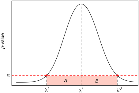
Figure 1. Construction of 100 × (1 − α) CI for λ* using the inverse probability method. The x-axis corresponds to the plausible values of λ in Equation (4), the y-axis to the p-value of the normality test, and the horizontal dotted line the type I error probability, α. It is worth mentioning that the relationship between λ and the p-value of the normality shown here is for illustration purposes only.

3.3. Selection of a Normality Test: Combined p-values

Several normality tests could be used in the steps described above, but their power depends on the sample size and the type of distribution the data resembles [31]. An automated approach to circumvent the job of selecting a normality test would be to fit several potential parent distributions to the λ_j-transformed data, find the distribution that gives the best fit (e.g., the lowest Akaike's Information Criterion [AIC]), and then choose the normality test with the highest power against that distribution. The drawback of this approach is there are also many candidate distributions that could be fitted to the data and not all of them have been studied in the context of normality tests. In other words, the power of all normality tests against all probability distributions is unknown.

A more parsimonious approach would be to use the combined p-value of a selected number of normality tests. Approximately 40 different types of normality tests exist [32] all of which can be coarsely classified in three categories: (i) regression/correlation-, (ii) empirical distribution function-, and (iii) measure of moments-based tests [31]. Thus, choosing an equal number of tests from each category would enable an educated assessment of the normality of a data set whose likely parent distribution is unknown. In this article, we used the Shapiro–Wilk (SW) and Shapiro–Francia (SF) tests from category (i), Kolmogorov–Smirnov (KS) and Anderson–Darling (AD) from category (ii), and Doornik–Hansen (DH) and robust Jarque–Bera (rJB) from category (iii).

Some of the methods proposed for the combination of p-values include Fisher's, Tippet's, Liptak's, Sidak's, Simes's, Stouffer's (see [33], for a review), and Vovk's [34]. In this article, we chose Stouffer's method because (i) it is more powerful and precise than others methods for combining p-values [35, 36]; and (ii) its simplicity by Z-transforming a set of p-values obtained from independent tests.

Using the Stouffer's method, the combined p-value of M independent statistical tests is

$\begin{array}{ll}{p}_{\text{combined}}=1-{\Phi }^{-1}(Z_S),& \left(8\right)\hfill \end{array}$

with

$\begin{array}{ll}{Z}_S=\frac{{\displaystyle {\sum }_{m=1}^M}{w}_m{Z}_m}{\sqrt{{\displaystyle {\sum }_{m=1}^M}{w}_m^2}}·& \left(9\right)\hfill \end{array}$

In the expressions above, Φ is the cumulative standard normal distribution, w_m is the weight of the mth study, and Z_m is the quantile of the standard normal distribution associated with p-value of the m statistical test, m = 1, 2, …, M.

Now, suppose M normality tests are chosen and used such that the pairs (λ_j, p_j)m are calculated, j = 1, 2, …, k, m = 1, 2, …, M. In addition, we combine p_{j, 1}, p_{j, 2}, …, p_{j, M} to obtain p_{j, combined}, j = 1, 2, …, k. Finally, using Stouffer's method, λ* is estimated as

$\begin{array}{ll}{\lambda }_{\text{combined}}^{*}=\left\{{\lambda }_j:p_{j,\text{combined}}=p_{(k),\text{combined}}\right\}& \left(10\right)\hfill \end{array}$

with p_{(k), combined} being the maximum of the combined p-values.

4. Examples

In this section, we illustrate the usefulness of our method by estimating λ* for two real data sets and compare the power of our method with that of the traditional MLE approach via a statistical simulation. Additionally, we provide an example demonstrating how well our method works in the case of a linear regression model.

4.1. Published Data

4.1.1. Example 1: Gesturing Movement Times

Salowitz et al. [37] measured the movement times of 13 autistic and 14 typically developing children when imitating hand/arm gestures and performing mirror drawing. Figure 2A represents the movement times of the autistic children when their task consisted of imitating a variety of gestures performed by a person in a video¹. The authors used a logarithmic transformation (λ = 0, Figure 2B) to normalize the movement times. It is clear from Figure 2B that such transformation achieves normality for most of the tests under consideration. However, the λ suggested by our method using the combination of p-values (λ* = 0.332, 95%CI = [−0.039, 0.707]) leads to a transformation with increased chances of passing most normality tests (see Figures 2B,C).

FIGURE 2

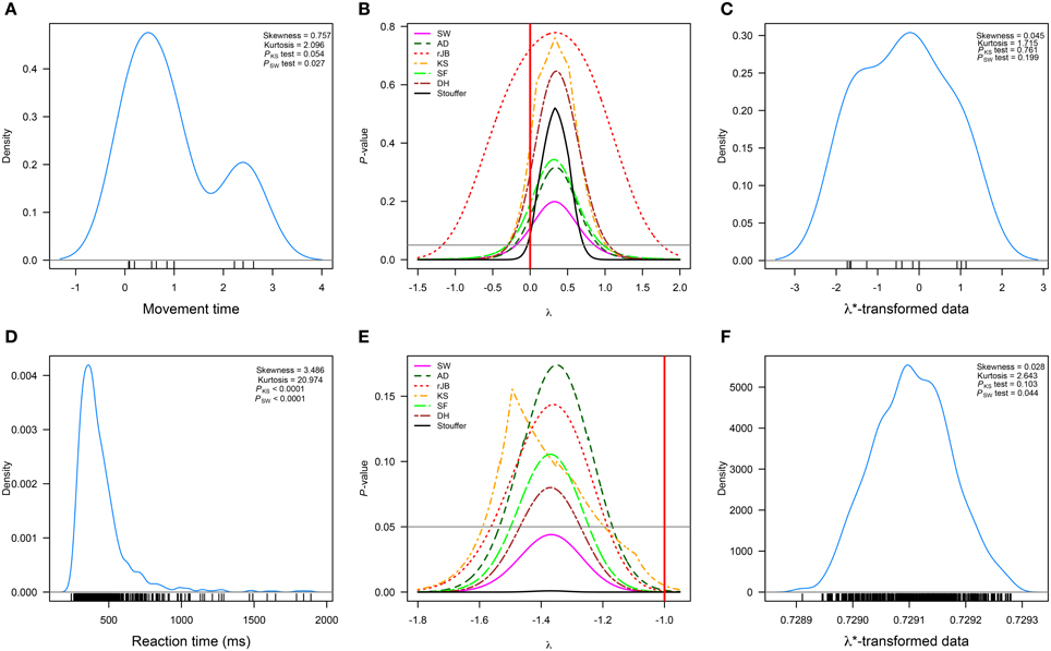
Figure 2. Published data sets in which the Box–Cox transformations was used. (A–C) correspond to the data (n = 13) analyzed in Salowitz et al. [37]; (D–F) to a set of observations (n = 917) analyzed in Marzouki et al. [38]. (A,D) correspond to the real data; (B,E) to the p-values of six normality tests and the Stouffer method as a function of λ; and (C,F) to the ${\lambda }_{\text{combined}}^{*}-$transformed data sets. The horizontal line represents α = 0.05, and the red vertical line the value of λ used by the researchers. Measures of skewness and kurtosis are also shown along with the p-values of the Kolmogorov–Smirnov (P_KS test) and Shapiro–Wilk (P_SW test) normality tests. rJB, robust Jarque–Bera; KS, Kolmogorov–Smirnov; DH, Doornik–Hansen; SW, Shapiro–Wilk; AD, Anderson–Darling; SF, Shapiro–Francia.

4.1.2. Example 2: Consonant Classification Times

Marzouki et al. [38] investigated whether information from a prime stimulus can be integrated with a target stimulus despite the two stimuli appearing at different spatial locations. In order to do so, five participants were asked to classify a set of target consonants as being a consonant or a pseudo-consonant (i.e., visual modifications of the target consonant). Target consonants appeared on seven different locations on the computer screen along the horizontal meridian. In one condition, consonants were primed by consonants and in the other consonants were preceded by pseudo-consonants. Participants repeated this task over five sessions during two blocks. Figure 2D represents the reaction times when consonants were preceded by consonants and when such pairings were presented on the extreme left area of the screen. The researchers used λ = −1 to normalize the results. As shown in Figure 2E, this value of λ would not lead to a successful normalization.

A similar result is obtained only when the SW normality test and the combined p-value approach are used with our method. However, the value ${\lambda }_{\text{DH}}^{*}=-1.3703$ (95%CI = [−1.469, −1.272]) transforms the data such that most normality tests, but SW, judge it as normal (Figure 2F shows the data transformed with this λ).

These two data sets further show that different normality tests can give different results regarding the normality of a specific data set and this is particularly evident in the difference between p-values given by the KS and SW tests. Specifically, the SW test is much more stringent than the KS test even when the data is assessed as normal by other normality tests (see the p-values in Figures 2A,F, as well as the results shown in the second column of that figure). The fact that normality tests give such different results simply reflects their power against different types of distributions and sample sizes [39]. Due to such a discrepancy in results, methods of combining p-values are helpful in gauging a p-value that would represent the normality of a specific data set as evaluated by a set of selected normality tests. Although our method can rely on one normality test alone, we believe using combined p-values, specifically the Stouffer method, is a sound and safe way to estimate λ.

4.2. Normalizing Residuals in Linear Regression

Suppose an outcome y and a predictor x are measured, and that it is of interest to apply a Box–Cox transformation when fitting the linear model

$\begin{array}{ll}y={\beta }_0+{\beta }_{1}x+ϵ& \left(11\right)\hfill \end{array}$

where ϵ is the error term. For simplicity, we simulate n = 50 observations with x uniformly distributed on the interval (1, 10) and ϵ from an exponential distribution with parameter μ = 1. Under this setting, it is clear that the error term does not meet the usual regression assumptions.

We estimate the parameter of the Box–Cox transformation using both MLE and our p-value-based approach using the Stouffer's method. In the first case, the boxcox function in Venables and Ripley [40] was used, whereas for our method a function in R was programmed. For a fixed value of λ, this function applies the Box–Cox transformation on y, fits the regression model, calculates the residuals, applies a normality test and finally extracts the p-value of such a test. As shown in §3.1, the value of λ* will be that for which the p-value of the normality test is the highest.

The combined p-value approach was also utilized to find the value of λ MLE and that provided by our p-value-based approach (see §3.3, for more details). In the first case, ${\widehat{\lambda }}_{\text{combined}}^{\text{MLE}}=0.282$ and $p_{\text{combined}}^{\text{MLE}}=0.0755$, whereas ${\lambda }_{\text{combined}}^{*}=0.4514$ and p_combined = 0.7297 using our approach. Furthermore, a comparison of the symmetry (γ) and kurtosis (β) coefficients for the residuals of model (Equation 11) after transforming y using the values found with each method revealed the residuals produced by our method are more symmetric (γ_MLE = −0.31 vs. γ_combined = 0.097) and have a kurtosis closer to that of the normal distribution (β_MLE = 2.791 vs. β_combined = 3.089). The values of γ → 0, β → 3, and p_combined → 1 suggest that our method is efficient at normalizing the residuals of this regression model.

4.3. Simulated Data

Several probability distributions have been proposed in the literature to model positively-skewed data, such as reaction and response time data. Distributions such as the Log-Normal, Weibull, and Wald have been suggested as candidate parent distributions for these types of data. However, the most studied is the Ex-Gaussian (EG) distribution [39].

In order to determine the performance of the MLE of λ and our p-value-based approach, we conducted a simulation study in which data sets from three EG distributions with parameters θ₁ = (300, 20, 300), θ₂ = (400, 20, 200), and θ₃ = (500, 20, 100) were generated (referred to as EG₁, EG₂ and EG₃, respectively). These parameters were chosen because they represent three levels of skewness in the data ranging from high (θ₁) to low (θ₃). The probability densities of these EG distributions can be seen in Marmolejo-Ramos and González-Burgos [39].

We implemented the following algorithm in R:

1. For fixed i and n, draw a random sample of size n from the ith distribution, i = 1, 2, 3. Denote this sample as y = (y₁, y₂, …, y_n).

2. Let M be the total number of normality tests. Apply Equation (1) on y and estimate ${\widehat{\lambda }}_{\text{MLE}}$. Now, on the λ_MLE-transformed data, apply the M normality tests and determine $p_1^{\text{MLE}},p_2^{\text{MLE}},\dots ,p_M^{\text{MLE}}$, the p-values of the M normality tests. Further, combine these p-values using Equation (8) to obtain $p_{\text{combined}}^{\text{MLE}}$.

3. Determine the pairs $({\lambda }_m^{*},p_m^{*})$, m = 1, 2, …, M. Subsequently, for each value of λ_j in the sequence λ_L, λ₂, …, λ_U, combine the p-values of the M normality tests to obtain p_{j, combined}, j = 1, 2, …, k. From these p-values, obtain ${\lambda }_{\text{combined}}^{*}$ and p_combined.

4. Report n, ${\widehat{\lambda }}_{\text{MLE}},p_1^{\text{MLE}},p_2^{\text{MLE}},\dots ,p_M^{\text{MLE}},p_{\text{combined}}^{\text{MLE}}$, the pairs $({\lambda }_m^{*},p_m^{*})$, m = 1, 2, …, M, and $({\lambda }_{\text{combined}}^{*},p_{\text{combined}})$.

5. Repeat steps 1–4, B times.

For analysis purposes, the rejection rate (RR) of the M normality tests and the combined p-values were calculated for each method (MLE and p-value-based). The RR was defined as

$\begin{array}{ll}RR=B^{-1}{\displaystyle \sum _{b=1}^B}{I}_{\left\{p_b<\alpha \right\}}& \left(12\right)\hfill \end{array}$

where p_b is the p-value of the test under evaluation in the bth iteration (b = 1, 2, …, B), and I is an indicator variable. The proportion of normalization can be thus obtained as 1 − RR.

In the simulation set up, we used n = {10, 30, 50, 100, 500} as sample sizes and considered the Shapiro–Wilk (shapiro.test in R), Anderson–Darling (ad.test in Gross and Ligges [41]), robust Jarque–Bera (rjb.test in Gastwirth et al. [42]), Shapiro–Francia (sf.test in Gross and Ligges [41]), Kolmogorov–Smirnov (lillie.test in Gross and Ligges [41]), and Doornik–Hansen (normality.test1 in Wickham [43]) normality tests. The Box–Cox transformation parameter was estimated with the powerTransform function in the car package [44]. As suggested by Robey and Barcikowski [45], a total of B = 1000 iterations were used.

4.3.1. Results

Figures 3, 4 show the main results. For each of the normality tests when λ_MLE and the combined p-value approaches were used, no obvious differences in the proportion of normalization were shown. However, as shown in Figure 3C, combining the p-values given by the normality tests for both the MLE and our method showed a slightly better performance of our method over the MLE, particularly when n < 100 across the three distributions. Figures 3A,B further suggests that our method does a better job than the MLE at normalizing less skewed distributions (like EG₃).

FIGURE 3

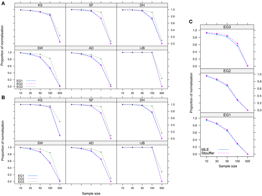
Figure 3. Proportion of normalization achieved by the (A) MLE and (B) p-value-based approaches for six normality tests in three Ex-Gaussian distributions, and (C) all p-values of the normality tests are combined using Stouffer's method. Abbreviations as in Figure 2.

FIGURE 4

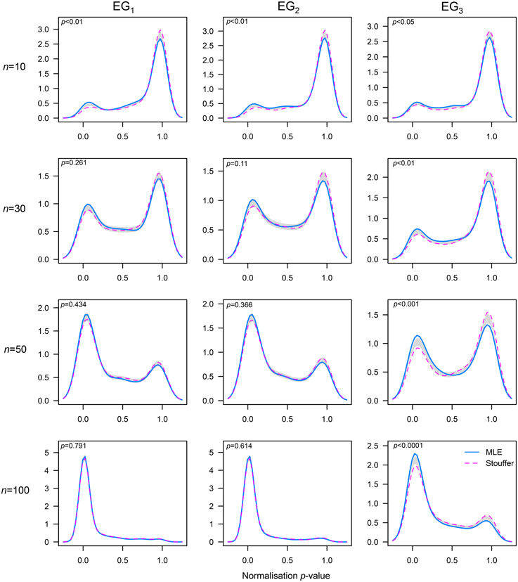
Figure 4. Comparison of probability densities between the MLE and Stouffer–combined p-value approaches to estimate λ. A permutation test of equality with n_boot = 1000 samples was utilized (see [48], for details). The x-axis represents the p-value obtained by combining six normality tests using the Stouffer's method; the support of the p-values is the interval (0, 1). Results for the sample sizes n = 10, 30, 50, and 100 are shown by row. The gray band represents the 95% CI for the difference between densities.

In order to formally determine differences between the methods tested, we compared the probability densities of the combined p-values obtained in the simulation. The results corroborated that our method performed better than the MLE method at normalizing non-normal distributions with low skewness across the sample sizes tested (see the third column in Figure 4). Additionally, this analysis showed that our method outperformed the MLE when distributions had mild (like EG₂) to high (like EG₁) levels of skewness and very small sample sizes (e.g., n = 10).

5. Discussion and Conclusions

The combined p-value approximation provides a better way of finding the appropriate λ for achieving normality since it considers the degree of agreement between the λ-transformed data and the normal distribution. If the p-value is sufficiently larger for more than one value of λ, we conclude that there is no way to guarantee normality with a single value of λ using our methodology; however this scenario seems unlikely. Although in our current implementation (see Appendix) of the proposed method it is not possible to select an optimal grid to search, we suggest exploring intervals and elements within these intervals to obtain a more precise value of λ*. Further implementations should include adaptive- and/or random-based search methods [46, 47]. Despite this, we believe that our methodology provides a new, easy-to-use and robust tool to help the data analyst decide which value of λ needs to be used in order to transform any data set so that its normality is guaranteed.

The results of the simulation study suggest that our method seems to be an improvement in the search of a λ in order to achieve normality, and posit topics for future investigation. The value of λ* can be affected by (i) the number and type of normality tests employed and (ii) the way the combined p-value is computed. It is important to recall that all available methods of combining p-values need the p-values given by independent tests, in our case normality tests. Although six normality tests from three different categories were used, it is tenable that if more tests are included in the estimation of the combined p-values, the results might be somewhat different. Indeed, results can be dramatically different if tests from only one or two categories are included in the computations. On the other hand, the estimation of the combined p-values is another aspect that plays a key role. We used the Stouffer's method based on its neat properties. However, the statistical properties of λ* and the power of other methods which combine p-values remain to be elucidated.

An issue in relation to the strength of our method is related to the parent distribution representing the data. It is clear that as the sample size increases, the normalization of the data becomes more challenging (see Figure 3), but also the type of distribution can add an extra challenge to the success of the transformation. Although we employed the Ex-Gaussian distribution, a type of untruncated continuous distribution, our method needs to be tested with other classes of non-normal distributions such as those used to model count and Likert-type data (be it truncated discrete or continuous) in the context of transformations (see [49] for count data, and [50–52] for Likert-type data). These ideas also apply to linear regression. That is, further testing is needed to evaluate the ability of our method to normalize residuals coming from regression models in which other non-normal distributions are used to represent the error term and outcome in the model, and when high leverage points or heteroskedasticity are present. It is also important to recall that the Yeo-Johnson transformation [30] should be used instead of the Box–Cox transformation when negative values are present in the data.

Finally, it is important to quantify how our p-value-based approach (to estimate λ) is affected by outliers. Although it is well-known that the traditional Box–Cox transformation is affected by outliers [7, 8], it remains to be elucidated if this is the case when our p-value-based approach is used. One way of addressing this issue would be to carry out a simulation study in which the underlying distribution of both the data and outlier generating process are known, and a fixed number of outliers are introduced to the uncontaminated data. Subsequently, an outlier detection method could be applied to the combined data (i.e., uncontaminated data + outlier observations) and the number of outliers detected would be further compared with that initially introduced. In fact, we have recently found that an outlier detection procedure known as the Ueda's method [53] is more likely to detect outliers when the data's distribution becomes more skewed and asymmetric [54]. Using the Ueda's method for the quantification of outliers affecting distributions transformed via the approach proposed herein is a topic for future investigation.

The application of our method in situations when the researcher has more than one vector of data to be transformed is important. This is the case, for instance, of reaction times measured on the same group of participants over x number of experimental conditions, and it is of interest to use a One-Way repeated measures ANOVA. By using our method and calculating the 95%CI around λ*, we argue that the user has a range of λs to select from in order to achieve, or approximate, the normality of those vectors obtained in each experimental condition. Further, it is possible that these CIs overlap with each other, and that a common λ* can successfully transform all vectors. This same idea would apply to a hypothetical case in which different participants are allocated to different experimental conditions and a One-Way independent measures ANOVA is to be used to analyse the data. Hence, we believe that the method proposed here is an improvement on the estimation of λ in the Box–Cox transformation and can be used by any researcher dealing with data that needs to meet the normality assumption.

Conflict of Interest Statement

The authors declare that the research was conducted in the absence of any commercial or financial relationships that could be construed as a potential conflict of interest.

Acknowledgments

The authors are particular grateful to Drs. Yousri Marzouki and Nicole Salowitz for sharing their data sets and answering questions on specific analytical aspects we needed to clarify. We also thank Nathan de Heer, Rosie Gronthos and La Patulya for proofreading the document. JV was supported by the Eccles Scholarship in Medical Sciences, the Fenner Merit Scholarship and the Australian National University (ANU) High Degree Research Scholarship. The first author is thankful to Dr. Mauricio Arcos-Burgos from ANU for his unconditional support.

Footnotes

1 ^See [37], for details of the computation of the movement times.

References

1. Mewhort DJK. A comparison of the randomization test with the F test when error is skewed. Behav Res Methods (2005) 37:426–35. doi: 10.3758/BF03192711

PubMed Abstract | CrossRef Full Text | Google Scholar

2. Feng C, Wang H, Lu N, Chen T, He H, Lu Y, et al. Log-transformation and its implications for data analysis. Shang Arch Psychiat. (2014) 26:105–9. doi: 10.3969/j.issn.1002-0829.2014.02.009

PubMed Abstract | CrossRef Full Text

3. Marmolejo-Ramos F, Cousineau D, Benites L, Maehara R. On the efficacy of procedures to normalise Ex-Gaussian distributions. Front Psychol. (2015) 5:1548. doi: 10.3389/fpsyg.2014.01548

PubMed Abstract | CrossRef Full Text | Google Scholar

4. Abelson RP. Statistics as Principled Argument. Mahwah, NJ: Psychology Press (1995).

Google Scholar

5. Kliegl R, Masson MEJ, Richter EM. Linear mixed model analysis of masked repetition priming. Vis Cognit. (2010) 18:655–81. doi: 10.1080/13506280902986058

CrossRef Full Text | Google Scholar

6. Olivier J, Norberg MM. Positively skewed data: revisiting the Box-Cox power transformation. Int J Psychol Res. (2010) 3:68–75.

Google Scholar

7. Box GEP, Cox DR. An analysis of transformations. J R Stat Soc B (1964) 26:211–52.

Google Scholar

8. Sakia RM. The Box-Cox transformation technique: a review. J R Stat Soc D (1992) 41:169–78. doi: 10.2307/2348250

CrossRef Full Text | Google Scholar

9. Li P. Box-Cox Transformations: An Overview. Department of Statistics, University of Connecticut (2005). Available online at: http://tinyurl.com/pli2005

10. Tukey JW. The comparative anatomy of transformations. Ann Math Stat. (1957) 28:602–32. doi: 10.1214/aoms/1177706875

CrossRef Full Text | Google Scholar

11. Cook RD, Wang PC. Transformations and influential cases in regression. Technometrics (1983) 25:337–43. doi: 10.1080/00401706.1983.10487896

CrossRef Full Text | Google Scholar

12. Carroll RJ, Ruppert D. Transformations in regression: a robust analysis. Technometrics (1985) 27:1–12. doi: 10.1080/00401706.1985.10488007

CrossRef Full Text | Google Scholar

13. Lawrence AJ. Regression transformation diagnostics using local influence. J Am Stat Assoc. (1988) 83:1067–72. doi: 10.1080/01621459.1988.10478702

CrossRef Full Text | Google Scholar

14. Kim C, Storer BE, Jeong M. A note on Box-Cox transformation diagnostics. Technometrics (1996) 38:178–80.

Google Scholar

15. Tsai C, Wu X. Transformation-model diagnostics. Technometrics (1992) 34:197–202. doi: 10.1080/00401706.1992.10484908

CrossRef Full Text | Google Scholar

16. Sweeting TJ. On the choice of prior distribution for the Box-Cox transformed linear model. Biometrika (1984) 71:127–34. doi: 10.1093/biomet/71.1.127

CrossRef Full Text | Google Scholar

17. Taylor JMG. Power transformations to symmetry. Biometrika (1984) 72:145–52. doi: 10.1093/biomet/72.1.145

CrossRef Full Text | Google Scholar

18. Hinkley D, Runger G. On quick choice of power transformation. J R Stat Soc C (1984) 79:302–9.

Google Scholar

19. Robinson PM. The estimation of transformation models. Int Stat Rev. (1993) 61:465–75. doi: 10.2307/1403756

CrossRef Full Text | Google Scholar

20. Carroll RJ, Ruppert D. On prediction and the power transformation family. Biometrika (1981) 68:609–15. doi: 10.1093/biomet/68.3.609

CrossRef Full Text | Google Scholar

21. Collins S. Prediction techniques for Box-Cox regression models. J Bus Econ Stat. (1991) 9:267–77.

Google Scholar

22. Tsai C, Wu X. Diagnostics in transformation and weighted regression. Technometrics (1990) 32:315–22. doi: 10.1080/00401706.1990.10484684

CrossRef Full Text | Google Scholar

23. Dagenais MG, Dufour J. Pitfalls of rescaling regression models with Box-Cox transformations. Rev Econ Stat. (1994) 76:571–5. doi: 10.2307/2109981

CrossRef Full Text | Google Scholar

24. Linnet K. Testing normality of transformed data. J R Stat Soc C (1988) 37:180–6. doi: 10.2307/2347337

CrossRef Full Text | Google Scholar

25. Foster AM, Tian L, Wei LJ. Estimation for the Box-Cox transformation model without assuming parametric error distribution. J Am Stat Assoc. (2001) 96:1097–101. doi: 10.1198/016214501753208753

CrossRef Full Text | Google Scholar

26. Casella G, Berger RL. Statistical Inference. Pacific Grove, CA: Duxbury Press (2001).

Google Scholar

27. Cheng RC, Traylor L. Non-regular maximum likelihood problems. J R Stat Soc B (1995) 57:3–44.

Google Scholar

28. Hernandez F, Johnson RA. The large-sample behavior of transformations to normality. J Am Stat Assoc. (1980) 75:855–61. doi: 10.1080/01621459.1980.10477563

CrossRef Full Text | Google Scholar

29. R Development Core Team. R: A Language and Environment for Statistical Computing. Vienna (2014). Available online at: http://www.R-project.org/

30. Yeo I, Johnson R. A new family of power transformations to improve normality or symmetry. Biometrica (2000) 87:954–9. doi: 10.1093/biomet/87.4.954

PubMed Abstract | CrossRef Full Text | Google Scholar

31. Romão X, Delgado R, Costa A. An empirical power comparison of univariate goodness-of-fit tests for normality. J Stat Comput Simul. (2010) 80:545–91. doi: 10.1080/00949650902740824

CrossRef Full Text | Google Scholar

32. Razali NM, Wah YB. Power comparison of some selected normality tests. In: Proceedings of the Regional Conference on Statistical Sciences (2010). 126–38.

33. García EK, Correa JC, Vélez JI. Combinación de pruebas de hipótesis independientes para proporciones: un estudio de simulación. In: Proceedings of the IX International Colloquium in Statistics, Medellín (Colombia).

34. Vovk V. Combining p-Values via Averaging (2012). Available online at: http://arxiv.org/pdf/1212.4966.pdf

35. Whitlock MC. Combining probability from independent tests: the weighted Z-method is superior to Fisher's approach. J Evol Biol. (2005) 18:1368–73. doi: 10.1111/j.1420-9101.2005.00917.x

PubMed Abstract | CrossRef Full Text | Google Scholar

36. Zaykin DV. Optimally weighted Z-test is a powerful method for combining probabilities in meta-analysis. J Evol Biol. (2011) 24:1836–41. doi: 10.1111/j.1420-9101.2011.02297.x

PubMed Abstract | CrossRef Full Text | Google Scholar

37. Salowitz NM, Eccarius P, Karst J, Carson A, Schohl K, Stevens S, et al. Brief report: visuo-spatial guidance of movement during gesture imitation and mirror drawing in children with autism spectrum disorders. J Autism Dev Disord. (2013) 43:985–95. doi: 10.1007/s10803-012-1631-8

PubMed Abstract | CrossRef Full Text

38. Marzouki Y, Meeter M, Grainger J. Location invariance in masked repetition priming of letters and words. Acta Psychol. (2013) 142:23–9. doi: 10.1016/j.actpsy.2012.10.006

PubMed Abstract | CrossRef Full Text | Google Scholar

39. Marmolejo-Ramos F, González-Burgos J. A power comparison of various normality tests of univariate normality on Ex-Gaussian distributions. Methodology (2013) 9:137–49. doi: 10.1027/1614-2241/a000059

CrossRef Full Text | Google Scholar

40. Venables WN, Ripley BD. Modern Applied Statistics with S, 4th Edn. New York, NY: Springer (2002). Available online at: http://www.stats.ox.ac.uk/pub/MASS4

41. Gross J, Ligges U. nortest: Tests for Normality. R package version 1.0-2 (2012). Available online at: http://CRAN.R-project.org/package=nortest

42. Gastwirth JL, Gel YR, Hui WLW, Lyubchich V, Miao W, Noguchi K. lawstat: An R Package for Biostatistics, Public Policy, and Law. R package version 2.4.1. (2013). Available online at: http://CRAN.R-project.org/package=lawstat

43. Wickham P. normwhn.test: Normality and White Noise Testing. R package version 1.0. (2012). Available online at: http://CRAN.R-project.org/package=normwhn.test

44. Fox J, Weisberg S. An R Companion to Applied Regression, 2nd Edn. Thousand Oaks, CA: Sage (2011). Available online at: http://socserv.socsci.mcmaster.ca/jfox/Books/Companion

45. Robey RR, Barcikowski RS. Type I error and the number of iterations in Monte Carlo studies of robustness. Br J Math Stat Psychol. (1992) 45:283–8. doi: 10.1111/j.2044-8317.1992.tb00993.x

CrossRef Full Text | Google Scholar

46. Schumer M, Steiglitz K. Adaptive step size random search. Automat Control IEEE Trans. (1968) 13:270–6. doi: 10.1109/TAC.1968.1098903

CrossRef Full Text | Google Scholar

47. Schrack G, Choit M. Optimized relative step size random searches. Math Program. (1976) 10:230–44. doi: 10.1007/BF01580669

CrossRef Full Text | Google Scholar

48. Bowman AW, Azzalini A. R package sm: Nonparametric Smoothing Methods (version 2.2-5.4). University of Glasgow, UK; Università di Padova, Italia (2014).

49. O'Hara RB, Kotze DJ. Do not log-transform count data. Methods Ecol Evol. (2010) 1:118–22. doi: 10.1111/j.2041-210X.2010.00021.x

CrossRef Full Text | Google Scholar

50. Kaptein MC, Nass C, Markopoulos P. Powerful and Consistent Analysis of Likert-type Rating scales. In: Proceedings of the SIGCHI Conference on Human Factors in Computing Systems. CHI '10. New York, NY: ACM (2010). pp. 2391–4.

51. Nevill A, Lane A. Why self-report “Likert” scale data should not be log-transformed. J Sports Sci. (2007) 25:1–2. doi: 10.1080/02640410601111183

PubMed Abstract | CrossRef Full Text

52. Wu CH. An empirical study on the transformation of Likert-scale data to numerical scores. Appl Math Sci. (2007) 1:2851–62.

Google Scholar

53. Ueda T. A simple method for the detection of outliers. Electron J Appl Stat Anal. (2009) 2:67–76. doi: 10.1285/i20705948v2n1p67

CrossRef Full Text

54. Marmolejo-Ramos F, Vélez JI, Romão, X. Automatic detection of discordant outliers via the Ueda's method. J Stat Dist Appl. (2015) 2:8. doi: 10.1186/s40488-015-0031-y

CrossRef Full Text | Google Scholar

Appendix

  A Implementation in R
  ## load the necessary functions and packages
  if(!require(devtools)) install.packages(‘‘devtools‘‘)
  devtools:::source_url("http://bit.ly/1eY6ZP2")

  # simulated data
  set.seed()7
  y  <- rexp(50, 1/100)

  # find lambda* between -1 and 2 using the combined p-values (Stouffer's method)
  # and plotALL = TRUE the results
  res0  <- lambda_star(y, lambdas = seq(-0.2, 1, length = 500),
                                method = "combined", plotALL = TRUE)
  res0