Optimal Control Problems in Finite-Strain Elasticity by Inner Pressure and Fiber Tension

1. Introduction

We consider optimization problems for fully 3D non-linear (finite-strain) stationary elasticity models. The novelty of the proposed approach is that we use an inner pressure or an inner fiber tension as a driving force. Such internal forces are typical, for instance, for the motion of heliotropic plants, and for muscle tissue, respectively. Moreover, we consider non-standard objective functions, which describe either a preferred normal direction of part of the boundary in the deformed state, or which cause the deformed body to avoid a virtual obstacle.

To date, there are relatively few papers dealing with the optimal control of finite-strain elasticity problems. Apparently the first is Szefer [1], where a sensitivity analysis for the displacement and eigenvalues is presented for an abstract control-in-the-coefficients problem, based on formal calculations. Paper Givoli and Patlashenko [2] presents a problem setting in two dimensions with a standard tracking-type objective and volume loads as control. The authors of Ibrahimbegovic et al. [3] consider optimization problems for a non-linear beam model with a finite number of control variables, viz. forces and moments. The work closest to ours is Lubkoll et al. [4], where the authors consider the computation of optimal boundary forces together with a tracking-type objective for the displacement. Compared to their work, we use novel control loads and more elaborate objective functions.

The solution approach we pursue in this paper is based on an optimize–then–discretize paradigm. That is, we derive first-order optimality conditions and design our solution algorithm in a function space setting. Discretization by finite elements is carried out only to perform the individual steps inside the algorithm. Specifically, we employ a function-space limited-memory quasi-Newton method to tackle the optimization problem. The advantage of such an approach, which is another novelty in the context of optimal control of elasticity models, is that we can expect a mesh-independent performance of the algorithm. This is confirmed by our numerical experiments.

Let us emphasize that the rigorous analysis of the finite-strain forward problem, let alone the corresponding optimality conditions, is rather demanding, see for instance [4–6]. We therefore base our development of first-order optimality conditions on formal calculations. In the much simpler case of infinitesimal strain models, rigorous analytical results have been achieved in Manservisi [7], Lovíšek [8], Lovíšek and Králik [9], and Nestler [10].

Notation

We summarize here the notational conventions used throughout the paper. Generally, we denote vector-valued quantities by bold-face letters. As customary for finite-strain problems, we distinguish between the undeformed (reference) and deformed (current) domains, Ω and $\hat{\Omega }$. Quantities defined on the deformed domain are likewise denoted by the $\hat{}$ symbol. Table 1 summarizes the notations used.

TABLE 1

Table 1. Notations used throughout the paper.

2. The Forward Problem of Finite-Strain Elasticity

The modeling follows the approach of Ciarlet [6]. An undeformed mechanical body is defined by a bounded domain Ω ⊂ ℝ³, whereas the deformed body is described by the domain $\hat{\Omega }\subset {ℝ}^3$. Material points in the undeformed body (the reference configuration) are denoted by x ∈ Ω and their corresponding counterparts in the deformed body (the current configuration) by $\hat{x}\in \hat{\Omega }$, see Figure 1. The two configurations are linked by a sufficiently smooth, bijective function $\hat{X}:\Omega \to \hat{\Omega }$ such that $\hat{x}=\hat{X}(x)$. Its inverse is denoted by $X:\hat{\Omega }\to \Omega$.

FIGURE 1

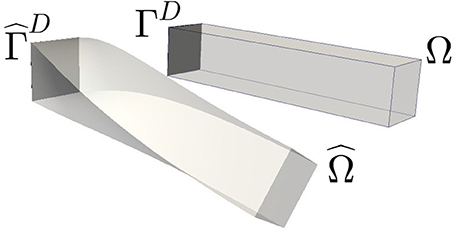
Figure 1. The undeformed body Ω (right) and the deformed body $\hat{\Omega }$ (left). Both have in common the portion of the boundary ${\Gamma }^D={\hat{\Gamma }}^D$ where the body is clamped.

The displacement U:Ω → ℝ³ is defined as $U(x):=\hat{X}(x)-x$ and the deformation gradient F:Ω → ℝ^{3 × 3} is

$\begin{array}{ll}F:=\mathrm{\text{D}}\hat{X}=\mathrm{\text{id}}+\mathrm{\text{D}}U,\hfill & \left(1\right)\end{array}$

or

$\begin{array}{l}F(x):=\mathrm{\text{D}}\hat{X}(x)=\mathrm{\text{id}}+\mathrm{\text{D}}U(x).\hfill \end{array}$

Herein, DU denotes the Jacobian (material derivative) with respect to x. By the chain rule, the material derivative of $\hat{U}=U◦X$ with respect to $\hat{x}$ is given by

$\begin{array}{ll}\widehat{\mathrm{\text{D}}}\hat{U}(\hat{x})=\widehat{\mathrm{\text{D}}}(U◦X)(\hat{x})=\left[(\mathrm{\text{D}}U)◦X(\hat{x})\right]\left[\widehat{\mathrm{\text{D}}}X(\hat{x})\right].\hfill & \left(2\right)\end{array}$

By the derivative of the inverse formula, and by writing x in place of $\text{X}(\hat{x})$, we obtain

$\begin{array}{ll}\widehat{\mathrm{\text{D}}}\hat{U}(\hat{X}(x))=\mathrm{\text{D}}U(x)F^{-1}(x).\hfill & \left(3\right)\end{array}$

2.1. Modeling of Loads and Variational Formulation

A deformation caused by applied loads can be modeled by a balance of forces in the deformed body. Commonly volume and boundary loads (e.g., gravitational forces) are considered in the literature. By contrast, we regard here two types of inner loads, namely an inner pressure and the tension of unidirectional fibers. For simplicity, gravitational and boundary forces are neglected here but they may be added to the formulation.

In this work, we consider the example from Figure 1 with hard clamping on a part Γ^D ⊂ ∂Ω of the boundary. This part of the boundary is identical in the undeformed and deformed bodies, i.e., ${\Gamma }^D={\hat{\Gamma }}^D$ holds. The clamping is expressed through the Dirichlet boundary condition

$\begin{array}{ll}U=0\text{\hspace{0.17em}on\hspace{0.17em}}{\Gamma }^D\text{\hspace{1em}and\hspace{1em}}\hat{U}=0\text{\hspace{0.17em}on\hspace{0.17em}}{\hat{\Gamma }}^D,\hfill & \left(4\right)\end{array}$

respectively. The function spaces ${U}$ and $\hat{{U}}$ denote the vector spaces of sufficiently smooth functions U:Ω → ℝ³ or $\hat{U}:\hat{\Omega }\to {ℝ}^3$, respectively, which satisfy Equation (4). In addition, natural (stress-free) boundary conditions are applied on the Neumann boundary ${\hat{\Gamma }}^N:=\partial \hat{\Omega }\backslash {\hat{\Gamma }}^D$. Naturally, the boundary stresses could be chosen non-zero as well.

2.1.1. Loads Modeling Turgor Pressure

Considering the pressure inside the body as a driving force is motivated by the turgor pressure occurring in so-called heliotropic plants. This pressure causes a deformation which allows these plants to follow the movement of the sun. The cause of the inner pressure is an osmotic potential inside the cells of the plant. This potential induces a local hydrostatic pressure, which can be written as the isotropic stress tensor $\hat{t}(\hat{x})\text{id}$ in the current configuration. The scalar field $\hat{t}:\hat{\Omega }\to ℝ$ describes the pressure value. The balance of forces in the current configuration then reads (cf. [6, pg. 69])

$\begin{array}{ll}\widehat{\text{div}}(\hat{T}(\hat{x})-\hat{t}(\hat{x})\text{id})=0\text{\hspace{1em}in\hspace{1em}}\hat{\Omega }.\hfill & \left(5\right)\end{array}$

The Cauchy stress tensor $\hat{T}(\hat{x})\in {ℝ}^{3\times 3}$ will be introduced below in Equation (8).

By multiplication of Equation (5) with an test function $\hat{V}\in {U}$ and integration by parts we obtain the variational equation (a.k.a. principle of virtual work),

$\begin{array}{ll}{\displaystyle {\int }_{\hat{\Omega }}}\hat{T}(\hat{x}):\hat{\text{D}}\hat{V}(\hat{x})\text{d}\hat{x}={\displaystyle {\int }_{\hat{\Omega }}}\hat{t}(\hat{x})\text{id}:\hat{\text{D}}\hat{V}(\hat{x})\text{d}\hat{x}\text{\hspace{0.17em}for\hspace{0.17em}all\hspace{0.17em}}\hat{V}\in \hat{U}.\hfill & \left(6\right)\end{array}$

The matrix inner product “:” is defined by A:B: = tr(A^⊤B). Note that the boundary condition $\hat{T}(\hat{x})-\hat{t}(\hat{x})\text{id}\hat{n}(\hat{x})=0$, which models the total stress normal to the surface ${\hat{\Gamma }}^N$ being equal to zero, has been incorporated into Equation (6). Moreover, we recall $\hat{V}=0\text{on}{\hat{\Gamma }}^D$. As a consequence, all boundary integrals vanish.

In order to transform the variational equation (Equation 6) to the reference configuration Ω, we apply the following rules: the current derivative $\hat{\text{D}}$ is transformed using the chain rule (Equation 3), i.e.,

$\begin{array}{ll}\hat{\text{D}}\hat{V}(\hat{X}(x))=\text{D}V(x)F^{-1}(x).\hfill & \left(7\right)\end{array}$

The Cauchy stress tensor $\hat{T}\in {ℝ}^{3\times 3}$ is related to the first Piola-Kirchhoff stress tensor T ∈ ℝ^{3 × 3}, see Equation (10) below, by the Piola transform

$\begin{array}{rc}T(x)=\left(\text{det}F(x)\right)\hat{T}(\hat{X}(x))F{(x)}^{-\top },\hfill & \left(\mathrm{8a}\right)\end{array}$

$\begin{array}{rc}\hat{T}(\hat{x})={\left(\text{det}F(X(\hat{x}))\right)}^{-1}T(X(\hat{x}))F{(X(\hat{x}))}^{\top },\hfill & \left(\mathrm{8b}\right)\end{array}$

cf. [6, Ch. 2.5]. We finally assume that the pressure of a cell does not depend on the current displacement but rather only on the material point itself, and hence we have $t(x)=\hat{t}(\hat{X}(x))$.

Using the transformation (Equation 8b) and the chain rule (Equations 7 and 6) becomes

$\begin{array}{ll}{\displaystyle {\int }_{\Omega }}T(x):\text{D}V(x)\text{d}x={\displaystyle {\int }_{\Omega }}t(x)\text{ cof }F(x):\text{D}V(x)\text{d}x\text{ for all }V\in U\hfill & \left(9\right)\end{array}$

with the cofactor matrix cofF: = (det F)F^−⊤.

The first Piola-Kirchhoff stress tensor T can be modeled with the help of an energy density w. A specific example will follow in Section 5. The relationship between T and the displacement U is eventually given by

$\begin{array}{ll}T(x)=w^{\prime }(F(x)):=\frac{\text{d}w}{\text{d}F}(F(x))\text{ with }F=\text{id}+\text{D}U.\hfill & \left(10\right)\end{array}$

Plugging Equation (10) into Equation (9) yields the final form of the variational formulation of the forward problem with inner pressure field t as applied load:

$\begin{array}{ll}\begin{array}{c}\text{Find }U\in {U}\text{such that}\hfill \\ {\displaystyle {\int }_{\Omega }}{w}^{\prime }(F(x)):\text{D}V(x)\text{d}x={\displaystyle {\int }_{\Omega }}t(x)\text{ cof }F(x):\text{D}V(x)\text{d}x\hfill \\ \text{\hspace{1em} \hspace{1em} \hspace{1em} \hspace{1em} \hspace{1em} \hspace{1em} for all }V\in {U}.\hfill \end{array}\hfill & \left(11\right)\end{array}$

2.1.2. Loads Modeling Fiber Tension

The second load presented in this paper is a spatially varying tension field m which acts on fibers along a given direction. The fiber direction a is a vector of unit Euclidean length, i.e., ∥a∥₂ = 1, which may also vary in space. Loads of this type are motivated for example by the tension of a muscle cell in a smooth, unidirectional muscle tissue. The tension m along the fiber direction a induces a principal stress in the direction a, which results in a stress tensor $\hat{m}(\hat{x})\hat{a}(\hat{x})\hat{a}{(\hat{x})}^{\top }$ at the material point $\hat{x}$ in the deformed configuration $\hat{\Omega }$, see for instance Odegard et al. [11]. Therefore, in this case the balance of forces reads

$\begin{array}{ll}\widehat{\mathrm{\text{div}}}\hat{T}(\hat{x})-\hat{m}(\hat{x})\hat{a}(\hat{x})\hat{a}{(\hat{x})}^{\top }=0\text{\hspace{1em} in }\hat{\Omega }.\hfill & \left(12\right)\end{array}$

Note that in contrast to the turgor pressure (Equation 5), the loads give rise to a stress component which is not of hydrostatic type.

Proceeding similarly as before in Equation (6), we construct the variational formulation in the current configuration, i.e.,

$\begin{array}{ll}{\displaystyle {\int }_{\hat{\Omega }}}\hat{T}(\hat{x}):\widehat{\mathrm{\text{D}}}\hat{V}(\hat{x})\mathrm{\text{d}}x={\displaystyle {\int }_{\hat{\Omega }}}\hat{m}(\hat{x})\hat{a}{(\hat{x})}^{\top }\widehat{\mathrm{\text{D}}}\hat{V}(\hat{x})\hat{a}(\hat{x})\mathrm{\text{d}}x\text{ for all }\hat{V}\in \hat{{U}}.\hfill & \left(13\right)\end{array}$

Next we transform this stress tensor to the reference configuration. First of all, we note that the fiber direction may have been rotated during the deformation which can be modeled by setting $\hat{a}=\frac{Fa}{\parallel Fa{\parallel }_2}$. To see this, consider a point x₁ ∈ Ω and a second point x₂ = x₁ + ta(x₁) with t > 0 in the direction of the fiber a(x₁). After the deformation the two points are moved to ${\hat{x}}_1=x_1+U(x_1)$ and ${\hat{x}}_2=x_2+U(x_2)$. The current (deformed) fiber direction $\hat{a}({\hat{x}}_1)$ then is

$\begin{array}{l}\begin{array}{c}{\displaystyle \underset{t\to 0}{\text{lim}}}\frac{1}{t}\left({\hat{x}}_2-{\hat{x}}_1\right)={\displaystyle \underset{t\to 0}{\text{lim}}}\frac{1}{t}\left(x_2+U(x_2)-x_1-U(x_1)\right)\hfill \\ ={\displaystyle \underset{t\to 0}{\text{lim}}}\frac{1}{t}\left(ta(x_1)+U(x_1+ta(x_1))-U(x_1)\right)\hfill \\ =a(x_1)+\text{D}U(x_1)a(x_1)=\left(\text{id}+\text{D}U(x_1)\right)a(x_1)\hfill \\ =F(x_1)a(x_1).\hfill \end{array}\hfill \end{array}$

Finally the current fiber direction is normalized and we obtain $\hat{a}=\frac{Fa}{\parallel Fa{\parallel }_2}$.

Secondly, we assume that the tension $\hat{m}$ scales such that any volume retains its total tension, i.e., it is independent of the volume change detF. The total tension along the fibers in an arbitrary volume ω ⊂ Ω is

$\begin{array}{l}{\displaystyle {\int }_{\omega }}{a}^{\top }\left(ma{a}^{\top }\right)a\text{\hspace{0.17em}d}x={\displaystyle {\int }_{\omega }}m(x)\text{d}x.\hfill \end{array}$

Analogously, the total tension along the fibers in the current configuration is

$\begin{array}{l}{\displaystyle {\int }_{\hat{\omega }}}{\hat{a}}^{\top }\widehat{(m}\hat{a}{\hat{a}}^{\top })\hat{a}\text{d}\hat{x}={\displaystyle {\int }_{\hat{\omega }}}\hat{m}\text{d}\hat{x}={\displaystyle {\int }_{\omega }}\hat{m}\widehat{(X}(x))\text{\hspace{0.17em}\hspace{0.17em}det }F(x)\text{d}x,\hfill \end{array}$

with $\hat{\omega }=\hat{X}(\omega )$. As the volume ω was arbitrary and both integrals are assumed to be equal, we have $m(x)=\hat{m}\hat{X}(x)\text{det}F(x)$, or $\hat{m}={(\text{det}F)}^{-1}m$. Using these transformation rules for the stress tensor $\hat{m}\hat{a}{\hat{a}}^{\top }$ and the Piola transform (Equation 8a) for $\hat{T}$ eventually yields the variational formulation on the reference domain,

$\begin{array}{l}\begin{array}{c}\text{Find }U\in {U}\text{such that}\hfill \\ {\displaystyle {\int }_{\Omega }}{w}^{\prime }(F(x)):\text{D}V(x)\text{d}x={\displaystyle {\int }_{\Omega }}m(x)\frac{a{(x)}^{\top }{F}^{\top }(x)\text{D}V(x)a(x)}{\parallel F(x)a(x){\parallel }_2^2}\text{d}x\hfill \\ \text{\hspace{1em} \hspace{1em} \hspace{1em} \hspace{1em} \hspace{1em} \hspace{1em} \hspace{1em} for all }V\in {U}.\hfill & \left(14\right)\end{array}\hfill \end{array}$

Remark 1. It is worthwhile noting that both variational problems (Equations 11 and 14) can also be obtained as the (formal) first-order necessary optimality condition of an energy minimization problem. That is, the forcing terms on the right hand sides of Equation (11) and Equation (14) can be attributed to a conservative force field. In the case of Equation (11), the appropriate energy minimization problem reads

$\begin{array}{l}\begin{array}{l}\text{Find }U\in {U}\mathrm{which}\mathrm{minimizes}\hfill \\ W^{(t)}(U,t):={\displaystyle {\int }_{\Omega }}w(\text{id}+\text{D}U(x))\text{d}x\hfill \\ -{\displaystyle {\int }_{\Omega }}t(x)\text{det}(\text{id}+\text{D}U(x))\text{d}x.\hfill & \left(15\right)\end{array}\hfill \end{array}$

Indeed, one easily verifies that Equation (11) coincides with

$\begin{array}{l}{W}_{,U}^{(t)}(U,t)\left[V\right]=0\mathrm{for}\mathrm{all}V\in {U},\hfill \end{array}$

i.e., the partial derivative of W^(t) at (U, t) w.r.t. U is equal to zero in all admissible directions V ∈ ${U}$.

In the case of fiber tension, one can verify in the same way that Equation (14) coincides with the first-order optimality condition of the energy minimization problem

Find U ∈ ${U}$ which minimizes

$\begin{array}{r}{W}^{(m)}(U,m):={\displaystyle {\int }_{\Omega }}w(\text{id}+\text{D}U(x))\text{d}x\hfill \\ -{\displaystyle {\int }_{\Omega }}m(x)ln\parallel (\text{id}+\text{D}U(x))a(x){\parallel }_2\text{d}x.\hfill & \left(16\right)\end{array}$

We shall utilize this observation in the solution of the forward problems, as detailed next.

2.2. Solution of the Forward Problem

The forward problems Equation (15) and Equation (16) will be jointly denoted by

$\begin{array}{ll}{\displaystyle \underset{U\in {U}}{min}}W(U,c)\hfill & \left(17\right)\end{array}$

The given load c is either the inner pressure t or the fiber tension m. A common method to solve this non-linear problem is a globalized Newtont's method applied to the first-order optimality conditions. At iterate U_ℓ, the search direction δU_ℓ is obtained from

$\begin{array}{ll}{W}_{,UU}(U_{\ell },c)\left[V,\delta U\right]=-W_{,U}(U_{\ell },c)\left[V\right]\text{\hspace{1em}for all }V\in {U}.\hfill & \left(18\right)\end{array}$

and a subsequent update U_ℓ+1 = U_ℓ + α_ℓδU_ℓ is performed. The number α_ℓ > 0 is the step length from a line search procedure for globalization. For the sake of completeness, we specify the concrete form of the derivatives in Equation (18) for our two examples. In case of the inner pressure t, we have

$\begin{array}{rc}{W}^{(t)}(U,t)={\displaystyle {\int }_{\Omega }}w(F)\text{d}x-{\displaystyle {\int }_{\Omega }}t\text{\hspace{0.17em}det }F\text{d}x\hfill & \left(\mathrm{19a}\right)\end{array}$

$\begin{array}{rc}{W}_{,U}^{(t)}(U,t)\left[V\right]={\displaystyle {\int }_{\Omega }}{w}^{\prime }(F):\text{ D}V\text{d}x-{\displaystyle {\int }_{\Omega }}t\text{ cof }F:\text{D}V\text{d}x\hfill & \left(\mathrm{19b}\right)\end{array}$

$\begin{array}{l}{W}_{,UU}^{(t)}(U,t)\left[V,\delta U\right]={\displaystyle {\int }_{\Omega }}{w}^{″}(F)\left[\text{D}V,\text{D}\delta U\right]\text{d}x\hfill \\ -{\displaystyle {\int }_{\Omega }}t(F^{-\top }:\text{D}\delta U)(\text{cof }F:\text{D}V)\hfill \\ -\left(F^{-1}\text{D}\delta U\right):\left(\text{D}{V}^{\top }\text{cof }F\right)\text{d}x\hfill & \left(\mathrm{19c}\right)\end{array}$

and in case of the fiber tension m, we get

$\begin{array}{rc}{W}^{(m)}(U,m)={\displaystyle {\int }_{\Omega }}w(F)\text{d}x-{\displaystyle {\int }_{\Omega }}mln\parallel Fa{\parallel }_2\text{d}x\hfill & \left(\mathrm{20a}\right)\end{array}$

$\begin{array}{rc}{W}_{,U}^{(m)}(U,m)\left[V\right]={\displaystyle {\int }_{\Omega }}{w}^{\prime }(F):\text{D}V\text{d}x-{\displaystyle {\int }_{\Omega }}m\frac{a^{\top }{F}^{\top }\text{D}Va}{\parallel Fa{\parallel }_2^2}\text{d}x,\hfill & \left(\mathrm{20b}\right)\end{array}$

$\begin{array}{r}{W}_{,UU}^{(m)}(U,m)\left[V,\delta U\right]={\displaystyle {\int }_{\Omega }}{w}^{″}(F)\left[\text{D}V,\text{D}\delta U\right]\text{d}x\hfill \\ -{\displaystyle {\int }_{\Omega }}m\frac{\left(a^{\top }\text{D}{V}^{\top }\text{D}\delta Ua\right)}{\parallel Fa{\parallel }_2^2}\hfill \\ -2m\frac{\left(a^{\top }{F}^{\top }\text{D}\delta Ua\right)\left(a^{\top }{F}^{\top }\text{D}Va\right)}{\parallel Fa{\parallel }_2^4}\text{d}x.\hfill & \left(\mathrm{20c}\right)\end{array}$

The spatial argument (x) was omitted here. Recall that F = id + DU holds.

It is well known that Newton's method for Equation (17) needs to be globalized, otherwise large Newton steps may lead to deformed bodies $\hat{\Omega }$ with regions of locally negative volume, i.e., det F(x) < 0. Globalization can be carried out by an incremental method [6, Ch. 6.10] which can be expanded with homotopy techniques. As an alternative, we use here a backtracking line search with an Armijo rule, applied to the energy W in Equation (17). This procedure ensures det F > 0.

3. Setting of the Optimal Control Problem

The goal of our optimal control problem is to determine a load (control) which affects a given desired deformation (state) of the work piece. The objective functions considered are of the form

$\begin{array}{ll}I(U,c)=Q(U)+\gamma P(c)\hfill & \left(21\right)\end{array}$

and they consist of a quality term Q for the state U and a penalty or cost term P for the control c. We consider the two types of control c that were mentioned in 2.1:

• inner pressure c = t : Ω → ℝ with the cost term $P(t)=\frac{1}{2}{\int }_{\Omega }t{(x)}^2\text{d}x$

• fiber tension c = m : Ω → ℝ with the cost term $P(m)=\frac{1}{2}{\int }_{\Omega }m{(x)}^2\text{d}x$

For the quality part Q we discuss three options, a standard tracking type functional and two new functionals, which are termed regional penalization and desired direction. In each case, we formulate the functional in the reference configuration and give its derivative with respect to the displacement field U, which is required for the numerical implementation.

Standard Tracking Type Objective Functional

The state U is matched against a desired state $U_{\text{des}}:\Omega \to {ℝ}^3$. The difference is measured in terms of

$\begin{array}{ll}{Q}^{\text{track}}(U)=\frac{1}{2}{\displaystyle {\int }_{\Omega }}\parallel U(x)-U_{\text{des}}(x)\parallel {}_2^2\text{d}x.\hfill & \left(22\right)\end{array}$

For later reference we note that the first derivative of Q with respect to U is

$\begin{array}{ll}{Q}_{,U}^{\text{track}}(U)\left[\delta U\right]={\displaystyle {\int }_{\Omega }}\delta U{(x)}^{\top }(U(x)-U_{\text{des}}(x))\text{d}x.\hfill & \left(23\right)\end{array}$

The tracking type functional Equation (22) is popular due to its simplicity but it has a drawback when used for deformation problems. Often it is not the displacement field which is the desired quantity but rather the deformed body $\hat{\Omega }$ itself, which can be achieved by many different displacement fields, and there is no natural candidate U_des among them. The following two new functionals can partly overcome these drawbacks.

Regional Penalization Functional

This quality functional can be used to avoid the deformed body to enter certain areas. To this end, every point in ℝ³ is assigned a penalty value given by means of a differentiable function q:ℝ³ → [0, ∞). Hence each material point $\hat{X}(x)=x+U(x)\in \hat{\Omega }$ of the deformed body carries the penalty value $q(\hat{x})$, and the total quality function can be formulated as

$\begin{array}{cc}{Q}^{pen}(U)={{{\displaystyle \int }}^{\text{}}}_{\widehat{\Omega }}q(\widehat{x})d\widehat{\Omega }={{{\displaystyle \int }}^{\text{}}}_{\Omega }q\left(x+U(x)\right)\text{ det }(\text{id}+DU(x))\text{d}x.& \left(24\right)\end{array}$

This formula could be differentiated directly to obtain the formal first-order derivative $Q_{\text{pen}}^{\prime }$, but a simpler representation without the derivative of q can be obtained with the help of Hadamard shape calculus (see for instance [12] and [13]), as provided by the following lemma. Note that the direction of differentiation δU takes the role of the perturbation vector field of the current configuration $\hat{\Omega }$ in the perturbation of identity approach.

Lemma 2. The derivative of Equation (24) in the direction of an admissible displacement field δU ∈ ${U}$ is given by

$\begin{array}{ll}{Q}_{,U}^{\text{pen}}(U)\left[\delta U\right]={\displaystyle {\int }_{\Gamma }}q(x+U(x))\delta U{(x)}^{\top }\text{ cof }F(x)n(x)\text{d}S.\hfill & \left(25\right)\end{array}$

Proof. Let δU ∈ ${U}$ be an arbitrary admissible perturbation of the deformation U. We seek a representation of the directional derivative $Q_{,U}^{\text{pen}}(U)\left[\delta U\right]$. The perturbation δU can be viewed as a perturbation of the deformed domain $\hat{\Omega }=\left\{\hat{x}=x+U(x),x\in \Omega \right\}$, that is ${\hat{\Omega }}_t:=\left\{x+U(x)+t\delta U(x),x\in \Omega \right\}$. Written in terms of the current configuration, that is ${\hat{\Omega }}_t=\left\{\hat{x}+t\delta \hat{U}(\hat{x}),\hat{x}\in \hat{\Omega }\right\}$, with the transformed perturbation $\delta \hat{U}(\hat{x}):=\delta U(X(\hat{x}))$. Following [12, Proposition 2.46], the shape derivative for a volume integral

$\begin{array}{l}{\displaystyle {\int }_{\hat{\Omega }}}q(\hat{x})\text{d}\hat{x}\hfill \end{array}$

is given by

$\begin{array}{ll}{\displaystyle {\int }_{\partial \hat{\Omega }}}q(\hat{x})\delta \hat{U}{(\hat{x})}^{\top }\hat{n}(\hat{x})\text{d}\hat{S},\hfill & \left(26\right)\end{array}$

with the outer normal $\hat{n}$ on the boundary $\partial \hat{\Omega }$. The next step is the transformation of Equation (26) back to the reference configuration Ω. The surface element becomes $\text{d}\hat{S}=\text{\hspace{0.17em}det }F(x)\parallel F{(x)}^{-\top }n(x){\parallel }_2\text{d}S$ and the outer normal $\hat{n}(\hat{X}(x))$ is $\frac{F{(x)}^{-\top }n(x)}{\parallel F{(x)}^{-\top }n(x){\parallel }_2}$, see [6, Theorem 1.7-1]. Inserting all of these and recalling cofF = (detF)F^−⊤, we obtain

$\begin{array}{l}{Q}_{,U}^{\text{pen}}(U)\left[\delta U\right]={\displaystyle {\int }_{\Gamma }}q(x+U(x))\delta U{(x)}^{\top }\text{ cof }F(x)n(x)\text{d}S\hfill \end{array}$

as claimed.                                                                        □

Desired Direction Functional

This quality term is motivated by the behavior of heliotropic flowers which point their flower heads toward the sun. Suppose that s ∈ ℝ³ is a normalized reference direction in the reference domain, e.g., the longitudinal direction of the stem below the flower head. Due to the deformation, this direction is rotated (and may be stretched) into the current direction $\hat{s}:\hat{\Omega }\to {ℝ}^3$. Thus, we have

$\begin{array}{ll}\hat{s}(\hat{X}(x))=F(x)s(x),x\in \Omega .\hfill & \left(27\right)\end{array}$

This current direction $\hat{s}$ is now matched against a desired direction $s_{\text{des}}(x):\Omega \to {ℝ}^3$, which leads to the quality term

$\begin{array}{ll}{Q}^{\text{dir}}(U)=\frac{1}{2}{\displaystyle {\int }_{\Omega }}\parallel F(x)s(x)-s_{\text{des}}(x){\parallel }_2^2\text{d}x.\hfill & \left(28\right)\end{array}$

Applying the chain rule and using F(x) = id + DU(x), we obtain the following representation of directional derivatives:

Lemma 3. The derivative of Equation (28) in the direction of an admissible displacement field δU ∈ ${U}$ is given by

$\begin{array}{ll}{Q}_{,U}^{\text{dir}}(U)\left[\delta U\right]={\displaystyle {\int }_{\Omega }}s{(x)}^{\top }\text{D}\delta U{(x)}^{\top }(F(x)s(x)-s_{\text{des}}(x))\text{d}x.\hfill & \left(29\right)\end{array}$

The optimal control problems we are considering are of the form

$\begin{array}{ll}\begin{array}{c}{\displaystyle \underset{(U,c)}{min}}I(U,c)=Q(U)+P(c)\hfill \\ \text{s.t. }U\in {U}\hfill \\ \end{array}\hfill & \left(30\right)\end{array}$

and the state equation W${}_{,U}^{(t)}(U,t)\left[V\right]=0$ is satisfied for all V ∈ ${U}$.

The specific problem depends on the choice of the control c (either inner pressure c = t, or fiber tension c = m), and the choice of the quality term (tracking type Q^track, desired direction Q^dir, or regional penalization Q^pen).

4. Solution of the Optimal Control Problem by a Reduced Quasi-Newton Method

We pursue here a so-called black-box approach to solve the optimal control problem (Equation 30), see Herzog and Kunisch [14] for a general overview. To this end, the state equation is eliminated by means of the control-to-state operator S:${C}$ → ${U}$, which assigns a solution U of the state equation for a given c, i.e.,

$\begin{array}{ll}U=S(c)\iff W_{,U}(U,c)\left[V\right]=0\text{\hspace{1em}for all }V\in {U}.\hfill & \left(31\right)\end{array}$

${C}$ and ${U}$ are suitable function spaces for the control and admissible displacements, i.e., incorporating the Dirichlet boundary condition (Equation 4). We note that the solution U may not be unique, cf. [6, Section 5.8] for examples. In practice, we evaluate S(c) using the globalized Newton procedure outlined in Section 2.2, and starting from a previous state for “neighboring” data c provides some control which solution is returned.

By means of the control-to-state operator, the optimal control problem Equation (30) reduces to the unconstrained problem

$\begin{array}{ll}{\displaystyle \underset{c}{min}}{I}^{\text{red}}(c)\text{\hspace{1em}with\hspace{1em}}{I}^{\text{red}}(c):=I(S(c),c)=Q(S(c))+P(c).\hfill & \left(32\right)\end{array}$

Next we state an adjoint-based representation of the derivative $I_{,c}^{\text{red}}(c)\in {{C}}^{*}$. First of all, an application of the chain rule yields

$\begin{array}{ll}{I}_{,c}^{\text{red}}(c)\left[\delta c\right]=Q_{,U}(U){[S}_{,c}(c)\left[\delta c\right]]+P_{,c}(c)\left[\delta c\right].\hfill & \left(33\right)\end{array}$

Here S_{, c}(c):${C}$→${U}$ is the linearized control-to-state operator, and through total differentiation of Equation (31), we see that δU = S_{, c}(c)[δc] is defined by

$\begin{array}{ll}{W}_{,UU}(U,c)\left[V,\delta U\right]+W_{,Uc}(U,c)\left[V,\delta c\right]=0\text{\hspace{1em}for all }V\in {U},\hfill & \left(34\right)\end{array}$

where U = S(c). We define the adjoint state Z ∈ ${U}$ as the solution of the adjoint equation

$\begin{array}{ll}{W}_{,UU}(U,c)\left[Z,V\right]+Q_{,U}(U)\left[V\right]=0\text{\hspace{1em}for all }V\in {U}.\hfill & \left(35\right)\end{array}$

Testing Equation (34) with V = Z and Equation (35) with V = δU, we get

$\begin{array}{l}\begin{array}{c}{W}_{,UU}(U,c)\left[Z,\delta U\right]+W_{,Uc}(U,c)\left[Z,\delta c\right]=0,\hfill \\ W_{,UU}(U,c)\left[Z,\delta U\right]+Q_{,U}(U)\left[\delta U\right]=0,\hfill \end{array}\hfill \end{array}$

and hence

$\begin{array}{l}{Q}_{,U}(U)\left[\delta U\right]=W_{,Uc}(U,c)\left[Z,\delta c\right].\hfill \end{array}$

With this identity and δU = S_{, c}(c)[δc], we reformulate the derivative (Equation 33) of I^red as

$\begin{array}{ll}{I}_{,c}^{\text{red}}(c)\left[\delta c\right]=W_{,Uc}(U,c)\left[Z,\delta c\right]+P_{,c}(c)\left[\delta c\right].\hfill & \left(36\right)\end{array}$

The representation (Equation 36) of the reduced derivative $I_{,c}^{\text{red}}$ can be used in derivative-based optimization algorithms. We employ here a quasi-Newton method with an inverse limited-memory BFGS-update shown in Algorithm 1 and Algorithm 2, compare, e.g., [15, ch. 7.2] or [16, ch. 4]. These methods are standard apart from their formulation in function space, which is why we state them here.

ALGORITHM 1

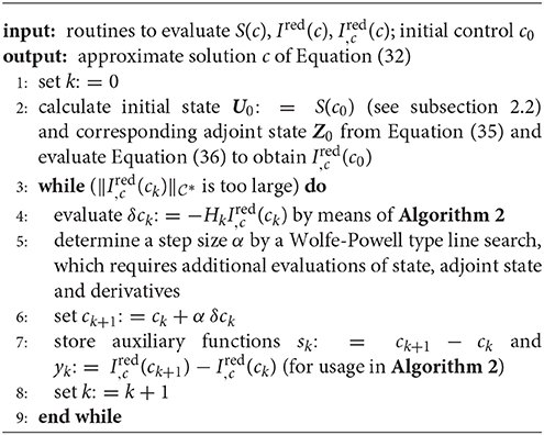
Algorithm 1. Quasi-Newton method

ALGORITHM 2

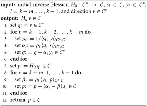
Algorithm 2. Inverse Limited-Memory BFGS procedure to evaluate H_kv ∈ ${C}$

For more details on the Wolfe-Powell line search method, see Nocedal and Wright [15, Alg. 3.5, p. 60]. Verification of the stopping criterion involves the evaluation of the norm of the derivative $I_{,c}^{\text{red}}(c_k)$ of the reduced objective in its native norm, i.e., the norm of the dual space ${C}$*. We provide more details on this in the discretized context in Section 5. The limited-memory BFGS method in function space is detailed in Algorithm 2. Note that only the m most recent pairs of data (s_k, y_k) are being used, and hence older data can be dropped upon storing s_k and y_k in step 7 of Algorithm 1, see Nocedal and Wright [15, ch. 6.1] for details. For a practical Wolfe-Powell line search procedure we refer to Nocedal and Wright [15, Algorithm 3.5].

4.1. Discretization and Linear Solver

We discretize our problem by a finite element method (FEM) on a hierarchy of uniformly refined tetrahedral meshes. We use continuous, piecewise linear ansatz functions (P₁) which satisfy the boundary conditions (Equation 4) for the displacement U and test functions, and piecewise constant functions (DG₀) for the control c, which may be either the inner pressure or the fiber tension. This defines discrete versions of the spaces ${U}$ and ${C}$.

In order to solve the linear systems (Equation 18) during Newton's method for the forward problem (Equation 17), we use a preconditioned truncated conjugate gradient method (tCG). Making use of the mesh hierarchy, we may employ a multigrid V-cycle with symmetric pre- and post-smoothing for the stiffness matrix of the linear elasticity model with Lamé constants λ, μ as a preconditioner. As an experimental (and faster) alternative, we applied in all numerical experiments below the multigrid V-cycle to the current Newton matrix in Equation (18), which is symmetric, but not necessarily positive definite. To overcome this potential problem, we terminate the tCG method in case the 'preconditioned norm' of the residual becomes negative. This safety occasionally became active in our numerical examples. Despite possible truncation, the search direction obtained in this way provides a greater reduction of the objective than the direction of steepest descent.

The (linear) adjoint system (Equation 35) is also solved with the tCG method with the same preconditioner as the forward problem. Note that, if the solution U of the forward problem was exact, then due to the energy minimization property, the operator W_{, UU}(U, c) is necessarily positive semi-definite. Consequently, even for slightly inexact forward solutions, the truncation safeties in the tCG method are unlikely to become active during the solution of adjoint systems, and in fact they never did in our numerical experiments.

5. Numerical Experiments

In this section we provide two examples which illustrate the use of the objective functionals Equation (24) and Equation (28), as well as the two control mechanisms by inner pressure and fiber tension introduced above. In both examples, we work with the polyconvex energy density w from Ciarlet [6, Ch. 4.10], i.e.,

$\begin{array}{ll}w(F)=a\parallel F{\parallel }_{\text{F}}^2+b\parallel \text{cof}F{\parallel }_{\text{F}}^2+c{(\text{det }F)}^2-dln(\text{det }F)+e,\hfill & \left(37\right)\end{array}$

where $\parallel A{\parallel }_{\text{F}}={(A:A)}^{1∕2}$ denotes the Frobenius norm, and a, b, c, d > 0 and e ∈ ℝ are material constants. The term ln(detF) can be viewed as a barrier term for the constraint det F > 0, which avoids local self-penetration. When considered a generalization of the energy density associated with a linear elastic material, which is described by the Lamé parameters λ, μ > 0, the parameters can be chosen according to

$\begin{array}{l}a=\frac{\mu }{2}-\frac{\lambda }{8},b=\frac{\lambda }{8},c=\frac{\lambda }{8},d=\mu +\frac{\lambda }{2},\hfill \\ e=-\frac{3\mu }{2}-\frac{\lambda }{8},\hfill \end{array}$

see Ciarlet [6, Ch. 4.10]. In the following numerical examples, we use the parameters (all in N mm⁻²)

$\begin{array}{l}\lambda =\frac{15}{26},\mu =\frac{5}{13},\text{\hspace{1em}i.e.,},a=\frac{25}{208},b=\frac{15}{208},c=\frac{15}{208},\hfill \\ d=\frac{35}{52},e=-\frac{135}{208},\hfill \end{array}$

which corresponds to a Young's modulus of E = 1 N mm⁻² and a Poisson's ratio of ν = 0.3 in the linear elasticity model obtained by a linearization of Equation (37). All lengths in the subsequent examples are given in mm as well. While the energy density (Equation 37) characterizes an isotropic material behavior, i.e., w(QF) = w(F) for rotation matrices Q, our approach applies to anisotropic materials as well.

Both our example problems are solved using the quasi-Newton method Algorithm 1. As initial inverse Hessian approximation H₀ in Algorithm 2, we use the inverse of the L² mass matrix in the control space, which is diagonal due to the choice of DG₀ elements. The relative stopping criterion for the quasi-Newton loop (with iteration counter k) is chosen to be

$\begin{array}{l}\parallel I_{,c}^{\text{red}}(c_k){\parallel }_{{{C}}^{*}}\le 10^{-4}\parallel I_{,c}^{\text{red}}(c_0){\parallel }_{{{C}}^{*}},\hfill \end{array}$

see step 3 of Algorithm 1, where the norm $\parallel ·{\parallel }_{{{C}}^{*}}$ is computed using the inverse of the diagonal L² mass matrix in the control space. The relative stopping criterion in Newton's method (with iteration counter ℓ) for the forward problem is

$\begin{array}{l}\parallel W_{,U}(U_{\ell },c_k){\parallel }_{P^{-1}}\le 10^{-6}\parallel W_{,U}(U_0,c_k){\parallel }_{P^{-1}},\hfill \end{array}$

with the norm introduced by the multigrid preconditioner. As mentioned before, we used a multigrid V-cycle applied to the current Newton matrix W_{, UU}(U₀, c_k) as preconditioner. The initial iterate U₀ is identical to the final iterate from the previous ((k−1)-st) quasi-Newton step, or U₀ in case k = 0. The relative stopping criterion for the residual in the tCG method (with iteration counter j) is implemented as

$\begin{array}{l}\parallel W_{,U}(U_{\ell },c_k)-W_{,UU}(U_{\ell },c_k)\delta U^{(j)}{\parallel }_{P^{-1}}\le 10^{-6}\parallel W_{,U}(U_{\ell },c_k){\parallel }_{P^{-1}}.\hfill \end{array}$

We use δU⁽⁰⁾ = 0 as initial guess.

5.1. Desired Direction with Inner Pressure Control

Example 6 (Part of a Heliotropic Flower Stem). We consider part of a hollow stem, i.e, a tube with an inner radius r₁ = 0.7, an outer radius r₂ = 1 and height h = 5. Dirichlet boundary conditions are applied at the bottom surface x₃ = 0. The control is the inner pressure t as in Equation (15) and it acts between the heights h = 0.5 and $\overline{h}=4.5$. We seek to align the top part of the stem, which has a reference direction s = (0, 0, 1)^⊤, with a desired direction s^des = (0, sin30°, cos30°)^⊤, which might represent the direction toward the sun, see Figure 2. Our objective is I(U, t) = Q^dir(U) + γP(t) with γ = 0.1.

FIGURE 2

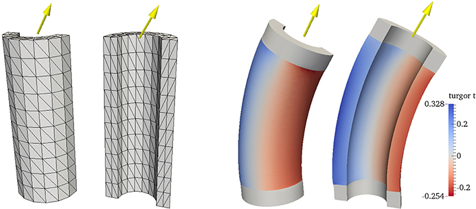
Figure 2. Left: Front and back view of a triangulation (on mesh level L = 0) of half of the hollow stem. The yellow arrow represents the desired direction s^des, which points toward the sun. Right: The solution of the optimal control problem. The inner pressure t is illustrated in the blue/red scale and the deformation is applied to the stem.

The solution is shown in Figure 2 and it illustrates the asymmetry in the frontal and rear regions of the stem. The positive turgor pressure (that is a high osmotic potential) expands the cells in the rear region while the negative turgor pressure (that is a low osmotic potential) shrinks the cells in the frontal region. As a consequence, the stem bends forward. The smooth distribution of the turgor pressure seems plausibel to occur in heliotropic flowers.

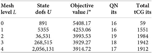
As for the numerical computation, the total number of iterations of the outer quasi-Newton and the inner tCG loops along with the number L of total mesh refinements can be found in Figure 3. We start the iteration with U = 0 and c = 0 on all meshes in order to observe the dependence of the method on the level of refinement. The truncation safeties in the tCG method with the experimental preconditioner occasionally became active during the solution of the forward system for all examples, but, as expected, only in early iterations of the quasi-Newton loop.

FIGURE 3

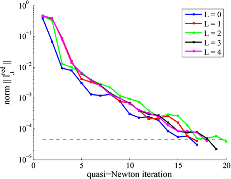
Figure 3. Numerical results from the quasi-Newton method for Example 6. Top: Number of iterations for various mesh refinement levels L. Bottom: Convergence behavior of the quasi-Newton method for various levels L.

The numerical experiment indicates that the number of iterations of the quasi-Newton method does not increase on finer meshes, and neither does the total number of tCG iterations. Also the overall convergence behavior is similar across the mesh refinement levels L = 0, 1, …, 4. This observed mesh-independent behavior is a result of the proper choice of norms and inner products (induced by the state and control function spaces), especially in the limited memory-BFGS update formula.

5.2. Regional Penalization with Fiber Tension Control

Example 7 (Bar and Plane). Consider a bar Ω = (0, 5) × (0, 1) × (0, 1) which is clamped at the left boundary Γ^D: = {0} × (0, 1) × (0, 1). We use as control the fiber tension m along the fiber direction a = (1, 0, 0)^⊤in the undeformed body. We seek a control m such that the deformed body avoids the half space

$\begin{array}{l}H:=\left\{x\in {ℝ}^3:x_1-x_3-2\ge 0\right\}.\hfill \end{array}$

We penalize the intrusion into this region by the quality functional Q^pen from Equation (24) with the penalty kernel

$\begin{array}{l}q(\hat{x})={\left[{\hat{x}}_1-{\hat{x}}_3-2\right]}_{\epsilon }^{+},\hfill \end{array}$

where ${\left[·\right]}_{\epsilon }^{+}$ is the smoothed positive part function ${\left[x\right]}_{\epsilon }^{+}:=\frac{1}{2}\left(\sqrt{x^2+{\epsilon }^2}+x\right)$. We choose the smoothing parameter ε = 10⁻⁴ and our objective is I (U, m) = Q^pen(U) + γP(m). The penalty kernel q is a smoothed version of ${\left[{\hat{x}}_1-{\hat{x}}_3-2\right]}^{+}$ which helps avoid numerical integration problems in the volume integral (Equation 24).

We considered several values for the penalty parameter γ in the numerical experiments. Figure 4 shows that an increase in γ puts more weight on the size of the control, which results in a more pronounced intrusion into the obstacle H. In case of γ = 0.1, the deformed body $\hat{\Omega }$ completely avoids the obstacle. Note that also the region near the obstacle is slightly penalized due to the use of ${\left[·\right]}_{\epsilon }^{+}$. Figure 5 shows the variation of the two parts in the objective w.r.t. γ.

FIGURE 4

Figure 4. Left: The undeformed body Ω and the half plane H from Example 7. The colored scaling indicates the value of the penalization function q. Right: The deformed body with the fiber tension in red (shorting of fibers) and blue (elongation) for γ = 0.1, 1, 10, 100.

FIGURE 5

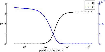
Figure 5. The values of the quality term Q and the penalty term P for various values of the penalty parameter γ.

6. Conclusions

In this manuscript we introduced two novel interior forces, inner pressure and fiber tension, which are integrated into the variational formulation of a non-linear elasticity problem. It has been shown that there exist corresponding energy potentials for these forces and thus we can employ a globally convergent line-search Newton method, which avoids local self penetration. We formulated an optimal control framework with two non-standard objective functionals, regional penalization and desired direction. Formal derivatives of these functionals are obtained partly by shape calculus.

As an optimization algorithm, we described a quasi-Newton method Algorithm 1 in a function space setting. Numerical experiments suggest that this method provides a mesh-independent convergence behavior, that is, there is an upper bound to the iteration numbers across all mesh sizes. The same applies to the Newton solver for the forward problem as well as the truncated CG method inside.

Author Contributions

RH suggested the research topic, contributed to the model formulation, verified the computations, suggested the algorithmic concepts. AG worked out the details of the algorithms, the derivative formulas, and carried out the numerical implementation and tests.

Conflict of Interest Statement

The authors declare that the research was conducted in the absence of any commercial or financial relationships that could be construed as a potential conflict of interest. The Handling Editor declared a shared affiliation, though no other collaboration, with one of the Reviewers [VR] and states that the process nevertheless met the standards of a fair and objective review.

Acknowledgments

This work was partly supported by the Federal Cluster of Excellence EXC 1075 “MERGE Technologies for Multifunctional Lightweight Structures” at Technische Universität Chemnitz. Funding through the German Science Foundation (DFG) is gratefully acknowledged.

References

1. Szefer G. Sensitivity and optimal control of elastic structures with distributed parameters. In: Bulirsch R, Miele A, Stoer J, Well KH, editors. Optimal Control (Oberwolfach, 1986). Vol. 95 of Lecture Notes in Control and Information Sciences. Berlin: Springer (1987). pp. 109–21.

2. Givoli D, Patlashenko I. Solution of static optimal control problems in non-linear elasticity via quadratic programming. Commun Numer Methods Eng. (2000) 16:877–90. doi: 10.1002/1099-0887(200012)16:12<877::AID-CNM384>3.0.CO;2-#

CrossRef Full Text | Google Scholar

3. Ibrahimbegovic A, Knopf-Lenoir C, Kučerová A, Villon P. Optimal design and optimal control of structures undergoing finite rotations and elastic deformations. Int J Numer Methods Eng. (2004) 61:2428–60. doi: 10.1002/nme.1150

CrossRef Full Text | Google Scholar

4. Lubkoll L, Schiela A, Weiser M. An optimal control problem in polyconvex hyperelasticity. SIAM J Control Opt. (2014) 52:1403–22. doi: 10.1137/120876629

CrossRef Full Text | Google Scholar

5. Ball JM. Convexity conditions and existence theorems in nonlinear elasticity. Arch Rat Mech Anal. (1976/1977) 63:337–403. doi: 10.1007/BF00279992

CrossRef Full Text

6. Ciarlet PG. Mathematical Elasticity. Vol. I. Vol. 20 of Studies in Mathematics and Its Applications. Amsterdam: North-Holland Publishing Co. (1988).

7. Manservisi S. An optimal control approach to an inverse nonlinear elastic shell problem applied to car windscreen design. Comput Methods Appl Mech Eng. (2000) 189:463–80. doi: 10.1016/S0045-7825(99)00302-3

CrossRef Full Text | Google Scholar

8. Lovíšek J. Optimal control problem of a nonhomogeneous viscoelastic reinforced plate with unilateral Winkler elastic foundation. ZAMM J Appl Math Mech. (2002) 82:599–617. doi: 10.1002/1521-4001(200209)82:9<599::AID-ZAMM599>3.0.CO;2-N

CrossRef Full Text | Google Scholar

9. Lovíšek J, Králik J. Optimal control for elasto-orthotropic plate. Control Cybern. (2006) 35:219–78. Available online at: http://matwbn.icm.edu.pl/ksiazki/cc/cc35/cc3523.pdf

10. Nestler P. Optimal thickness of a cylindrical shell under a time-dependent force. J Opt Theory Appl. (2013) 158:498–520. doi: 10.1007/s10957-012-0255-7

CrossRef Full Text | Google Scholar

11. Odegard GM, Haut Donahue TL Morrow DA, Kaufman KR. Constitutive modeling of skeletal muscle tissue with an explicit strain-energy function. J Biomed Eng. (2010) 130:061017. doi: 10.1115/1.3002766

PubMed Abstract | CrossRef Full Text | Google Scholar

12. Sokołowski J, Zolésio JP. Introduction to Shape Optimization. New York: Springer (1992).

13. Eppler K. On Hadamard Shape Gradient Representations in Linear Elasticity. Priority Program 1253, German Research Foundation (2010). Available online at: http://www.am.uni-erlangen.de/home/spp1253/wiki/index.php/Preprints

14. Herzog R, Kunisch K. Algorithms for PDE-Constrained Optimization. GAMM Rep. (2010) 33:163–76. doi: 10.1002/gamm.201010013

CrossRef Full Text | Google Scholar

15. Nocedal J, Wright S. Numerical Optimization. 2nd ed. New York: Springer (2006).

Google Scholar

16. Kelley CT. Iterative Methods for Optimization. Vol. 18 of Frontiers in Applied Mathematics. Philadelphia, PA: Society for Industrial and Applied Mathematics (SIAM) (1999).