Mimicking Directed Binary Networks for Exploring Systemic Sensitivity: Is NCAA FBS a Fragile Competition System?

1. Introduction

Advances in Information Technology have equipped scientists with unprecedented capabilities to create new systems as well as to peek into old systems in human societies and in nature. Scientific endeavors of collecting and mining diverse kinds of high frequency, sequencing and network data for better understanding on these new and old systems of interest are nearly overwhelming across all branches of science. Though methodological techniques on computing and analyzing data derived from such systems have progressed in many fronts in past decades, still the speed of progress on learning from data apparently lags far behind the speed of generating data. One of the key reasons behind this lagging phenomenon can be seen from the perspective of order and chaos, as described in Crutchfield [1]. Any physical system of scientific interest is simultaneously characterized by its deterministic structures and its randomness. Critically these two systemic characteristics are coupled with each other in unknown and complex fashions. This coupling relation is hardly simple, much less linear which contributes to the complexity of real world systems.

Within a complex system, Crutchfield [1] asked questions: What is a pattern? How do we come to recognize and compute patterns never seen before? He further asserted that quantifying the notion of pattern and formalizing the process of pattern discovery go right to the heart of physical science. To formalize a suitable process of pattern discovery in a target system, some knowledge and insights regarding the architecture of systemic complexity, which have been advanced several decades ago, become even more valuable than ever. For instance, Simon [2] argued that hierarchical organizations likely merge in the process of evolution as systems converge toward their stable states, while Anderson [3] brought out that the twin difficulties of scale and complexity are keys to understanding large and complex systems. Up to now much more light has been shed on complex systems. A series of interesting related work can be found in the journal Chaos's Focus Issue on “Randomness, Structure, and Causality: Measure of Complexity from Theory to Applications, see Crutchfield and Machta [4] and papers therein.

In this paper we not only heel to the insights of hierarchical and multiscale structures when formalizing a process of pattern discovery upon a real world complex system, but also we take one step further to make use the discovered systemic patterns for exploring systems' sensitivity. That is, after computing and discovering deterministic structures in the form of pattern hierarchy, we attempt to explore which scales of the hierarchical constructs are susceptible to perturbations within discovered reign of randomness. This perspective of coupling deterministic and stochastic macroscopic components on research of directed network is still missing in literature of statistical mechanics on complex networks, see Albert and Barabási [5]. In contrast, recent works on universal resilience patterns in complex network are primarily studied through multiple dimensional differential equations, see Barzel and Barabási [6] and Gao et al. [7]. Our data-driven exploration endeavors here should add one more dimension of systemic understanding from the perspective of control theory, in which a system's complexity is thought of being characterized by its robustness as well [8].

Here our focus is particularly placed on any system that can be represented or approximated by a directed binary network. For the purpose of concrete and real exposition, but without loss of generality, we employ the competitive system of the NCAA Football Bowl Subdivision (FBS) to illustrate our computational developments. A glimpse at the characteristics of a directed binary network is given as follows.

It can be mathematically represented by a non-symmetric square binary matrix. The directedness refers to its relational “flows” on each linkage beginning from one node and ending on another node. A collection of such flows make up ample quantities of flow-paths, also called dominance paths, of various lengths. It likely also contains cyclic flow-paths as loops of different lengths. In the sense of dominance, a cyclic flow-path indicates a piece of conflicting dominance information. In the NCAA example, flow-path cycles are prevalent. It is worth noting that this case is not universal. For instance, the Rhesus Macaque monkeys' Silent Bared Teeth (SBT) behavioral networks, as reported in Fujii et al. [9], have no such flow-cycles. That is, there is no ambiguity in any dominance relationship in the monkey society through the SBT behavior. In contrast the NCAA Football competitive system is much more complex in this aspect, since it indeed allows highly heterogeneous degrees of uncertainties among all possible node-pairs. As would be seen in sections below, such conflicting information is the primary source of computational complexity and difficulty in directed binary networks. Though this fact has long been recognized by animal scientists, who studied ranking structures in animal societies (see [10–14]), so far no theories are available to constitute optimal methodologies for extracting global structural patterns from directed binary network data (see [15]).

For expositional simplicity within the competition system of NCAA football, a directed binary network is represented by a binary “win-and-loss” matrix. And the symmetrized “win-and-loss” matrix, the sum of the transposed “win-and-loss” matrix with itself, is a symmetric undirected schedule matrix.

We attempt the pattern discovery by following steps. We first construct a dominance probability matrix by extracting all pairwise dominance potentials from the collection of dominance paths contained within an observed binary “win-and-loss” matrix. We then take this dominance probability matrix as a thermodynamic system, on which we build a Hamiltonian. As such we quantify the deterministic structure by the minimum energy ground state, or macrostate. Such a computable macrostate reveals a power hierarchy among all involved nodes. Another pattern structure, called the Parisi adjacency matrix, is computationally discovered from the schedule matrix via an approach also based on statistical mechanics, see Fushing et al. [16]. We then argue that this dominance probability matrix together with the computed Parisi adjacency matrix constitute the discovered randomness as another intrinsic stochastic component embedded within the directed binary network under study. Based on such a randomness component, we are able to propose a network mimicking algorithm to generate microstates that are indeed conforming the macrostate. The resultant microstate ensemble would be used as an operational platform for exploring systemic sensitivity. This series of computational development is exclusively illustrated upon 2 years of NCAA college football data from the 2012 and 2013 seasons.

2. Materials and Methods

2.1. Win-and-Loss Matrix

Let a directed binary network ${G}$(${W}$₀) be represented by a m × m binary win-and-loss matrix ${W}$₀ = [${W}$₀[i, j]] with ${W}$₀[i, j] = 1 meaning team i having one “win” over team j, and ${W}$₀[i, j] = 0 one “loss” to team j. The sum of ${W}$₀ and its transpose, ${{A}}_0={{W}}_0+{{W}}_0^T$, is termed the schedule matrix. ${A}$₀ is binary and symmetric.

The 2012 and 2013 NCAA college football schedules are shown in Figures 1A,B, respectively. There are 124(= m) teams in 2012, and 125 in 2013, competing in the two NCAA football examples. The majority of teams are divided into 10 conferences, such as Pac-12, Big-10, and SEC etc. with 6 independent teams. The ten block structures in Figure 1 show more intra-conference than inter-conference games. Each team plays 12 or 13 games without multiplicity against any opponent team. That is, if two teams meet, we have ${W}$₀[i, j] + ${W}$₀[j, i] = ${A}$₀[i, j] = ${A}$₀[j, i] = 1, so that they meet only once in the regular season. As a result, these two win-and-loss matrices are not only authentically binary, but also are rather sparse since there are in total fewer than 750 games played among more than 7500 possible team-pairs. Hence nine out of ten entries in both matrices are missing. In sharp contrast a dominance probability matrix computed below solely based on the two ${W}$₀ has nearly no missing entries.

FIGURE 1

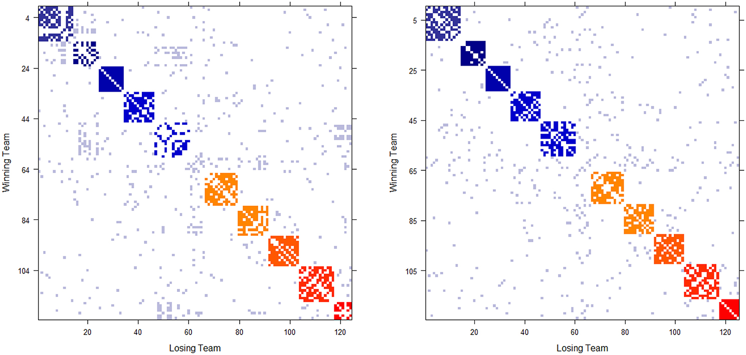
Figure 1. Schedule matrix ${A}$₀ of NCAA football data for the 2012 season (Left panel) and 2013 season(Right panel). The schedule matrix is composed of colored diagonal blocks marking the intra-conference games for the real conferences, and off-diagonal inter-conference games are marked in gray. The six independent teams account for the gap in the middle rows and columns. Conferences, from blue to red, are ACC, American, Big 12, Big Ten, Conference-USA, Independent schools, Mid-American, Mountain West, Pac 12, SEC, and Sun Belt.

2.2. Initial Beta Random Field

To begin, it is natural to ask: How much a win is worth in the sense of dominance? Formally, given the fact that ${W}$₀[i, j] = 1, what is the conditional probability that team i would win against team j in their next hypothetical encounter? Such a probability surely depends on the nature or uncertainty in outcome of the “game,” such as the NCAA football competitive landscape, as well as on their discrepancy of their winning potentials, which is intuitively related to the difference of their “true” ranking statuses. To mathematically formalize these thoughts, we propose to model such a conditional probability through a Beta random variable Be(w[i, j]α_{i, j} + 1, w[j, i]α_{i, j} + 1). This proposal relies on the fact that Be(w[i, j] + 1, w[j, i] + 1) is a Beta posterior distribution under a Bernoulli trial with Uniform prior U[0, 1] = Be(1, 1). And α_{i, j} would be computed in a data-driven fashion. The larger α_{i, j} value is, the distribution of Be(w[i, j]α_{i, j} + 1, w[j, i]α_{i, j} + 1) is more concentrated toward 1.

To compute α_{i, j} in a data-driven fashion, we consider the following decomposition α_{i, j} = α₀ + Δα_{i, j}, where α₀ accounts for the nature of NCAA football games, and Δα_{i, j} for the discrepancy of winning potentials between teams i and j. The α₀ is computed based on the overall triad-based transitivity, while Δα_{i, j} is based on their tree distance found in a classification hierarchy of all involving teams.

The triad-based transitivity on ${W}$₀ is computed as follows. Here an order-0, or a direct, dominance of (i, j) pair is referring to the case w[i, j] + w[j, i] = 1. If w[i, j] = 1, i is direct dominating j. An order-1 dominance path of (i, j) pair refers to the existence of one intermediate team-node k such that, either w[i, k] = 1, w[k, j] = 1 for the order-1 indirect dominance of i over j, or w[j, k] = 1, w[k, i] = 1 for j over i. Further a triad {i, j, k} is termed being coherent in dominance if i dominates j, i dominates k and k dominates j. For a triad of nodes having three directed edges, there are only two possibilities: being coherent or incoherent between the direct and the order-1 indirect dominance direction. Therefore as one of global features of ${W}$₀, the triad-based transitivity is defined as the proportion of coherent dominance, excluding all triads with fewer than three edges. The empirical proportion is denoted as $\widehat{T}({{W}}_0)$.

Then we heuristically equate the transitivity estimate $\widehat{T}({{W}}_0)$ to the dominance probability computed through an order-1 dominance path:

$\widehat{T}({{W}}_0)={\left(\frac{{\alpha }_0+1}{{\alpha }_0+2}\right)}^2$

where $\frac{{\alpha }_0+1}{{\alpha }_0+2}$ is the mean value of Be(α₀ + 1, 1).

Though this equation is rather simplistic, it works reasonably well when $\widehat{T}({{W}}_0)\ge 0.5$. For instance, if the empirical $\widehat{T}({{W}}_0)$ is calculated as 0.72, then the data-driven α₀ = 5.6. Then the random variable Be(5.6 + 1, 1) has its mean around 0.9 and variance less than 0.015. This context-dependent choice of Beta distribution is very different from Be(2, 1) with its mean 2∕3 and variance 0.056(= 1∕18) as used in Fushing et al. [17]. As the extreme case, if T(${W}$₀) = 1.0, the perfect transitivity, then α₀ = ∞. It means that the dominance probability is always 1.

We place one Beta random variable with distribution Be(α₀ + 1, 1) onto every (i, j)-entry of the m × m lattice where w[i, j] = 1, otherwise the entry is left blank. It is emphasized that the blanks, not Be(1, 1), are placed for entries without observed direct dominance, that is, for all (i, j) pairs with w[i, j] + w[j, i] = 0. The m × m matrix array of Beta random variables and blanks is called Beta Random Field in Fushing et al. [17].

This random field allows us to simulate random dominance paths mimicking the observed ones. This capability is critical for carrying out the “ensemble” idea for extracting the initial version of dominance probability matrix, from which the initial version of power structural hierarchy is derived, as will be discussed in the next subsection.

After the initial version of the power structural hierarchy is derived, tree distances for all pairs of nodes become available. We then estimate Δα_{i, j} for all (i, j) pairs having w[i, j] + w[j, i] = 1. Finally, refined versions of the dominance probability matrix and the power structural hierarchy are derived.

2.3. Initial Dominance Probability Matrix

The complexity of computing an initial dominance probability matrix, denoted as $P_D^{(0)}({{W}}_0)$ based on an observed win-and-loss matrix ${W}$₀, involves one critical front: to identify all of the locations of “real structural” blank entries under a nonparametric framework. Here a “real structural” blank entry refers to a pair of nodes without dominance relationship, not because of lack of data. This task becomes particularly difficult when the number of all possible pairs m(m − 1) ∕ 2 is large and the number of missing entries, w[i, j] + w[j, i] = 0 is overwhelming in ${W}$₀.

To resolve this critical computational issue, we devise an algorithm called the Trickling percolation process. Heuristically we make use of common percolation processes trickling within the Beta random field to explore and simulate as many dominance paths as possible. By performing a huge number of such percolation processes, we hope that collectively such percolating trajectories would be able to exhaustively visit every possible non-blank entries. Those entries completely missed by every single percolation processing should be reasonably taken as blank entries. At the same time the ensemble of simulated percolation trajectories is thought to achieve a uniform sampling of all possible dominance paths. Therefore any pair of nodes, which have dominance relationship, is sampled with pertinent frequencies in either dominance direction. The ratio of these two frequencies should properly reflect their dominance potential. The precise algorithmic description of the Trickling percolation process is given below.

2.3.1. Trickling Percolation Algorithm

TP-1: Consider a Markovian process to begin with a random initial node i₀ such that $\sum _{j=1}^m{w}_{i_0,j}>0$ and make a zero m × m matrix E and index k = 1;

TP-2: Select a candidate neighbor i_k with equal probability from the set of nodes {i|w_i0, i = 1, i = 1, .., m}(also excluding nodes already appeared in the Markovian process);

TP-3: Generate a random value p from Be(α₀+1, 1) and simulate a Bernoulli random variable X_ik ~ BN(p). If X_ik = 1, then count it as a “win,” otherwise a “loss.” Record the win or loss as order-0 dominance for the node-pair into entries (i₀, i_k) and (i_k, i₀) in matrix E.;

TP-4: If X_ik = 1, then add node i_k into the dominance path and let the Markovian process go to the TP-2 step with index k = k + 1. If it is loss, then a simulated dominance path ends, so is the Markovian process stops. Go to the next step;

TP-5: Transform all order-2, 3,.…of pairwise dominance along the Markovian simulated dominance path into order-0 pairwise dominance and record them into E.

Specifically the simulated dominance matrix E resulted from the Tricking percolation algorithm has 1's in the following collection of entries {(i_k, i_j)|k < j ≤ K, k = 0, 1, …, K} when a realized simulated Markovian dominance path is the sequence {i₀, i₁, … i_k, ….i_K, i_{K + 1}} with X_{iK + 1} = 0 and entries E[i_K, i_{K + 1}] = 0 and E[i_{K + 1}, i_K] = 1.

One simulation of the above Trickling percolation algorithm gives rise to one replication of simulated win-and-loss dominance matrix E. We construct a collection of a large number of replications of E′s matrices, and denote the matrix summing over the win-and-loss dominance matrix ensemble as ${E}$(${W}$₀). We then take the following ensemble average via an entry-wise ratio operation: for the (i, j) entry of matrix $\overline{D}({{W}}_0)$,

$\overline{D}({{W}}_0)\left[i,j\right]=\frac{{E}({{W}}_{\prime })\left[i,j\right]}{{E}({{W}}_{\prime })\left[i,j\right]+{E}({{W}}_{\prime })\left[j,i\right]}.$

This special ensemble average $\overline{D}({{W}}_0)$ pragmatically provides reasonable pairwise dominance probability for all potential dominance relationships possibly embedded within ${W}$₀. And very importantly, any blank in $\overline{D}({{W}}_0)$ reliably has no dominance relationships up to the extent of the percolating capability of Trickling percolation algorithm. Hence $\overline{D}({{W}}_0)$ is taken as a non-structural version of dominance probability matrix.

3. Results

The computed dominance probability matrix $\overline{D}({{W}}_0)$ from the previous section would be the basis for extracting systemic structures: namely, its deterministic structure and its randomness. It is noted that the deterministic structure is likely a composite structure comprised of multiple overlapping trees. To bring out and present such a structural composition in one single hierarchy can be rather complicated. Here we represent two global aspects of the deterministic structure of dominance: one power-ordering axis and one power hierarchy. It is also noted that the system's randomness is highly associated with the deterministic structure and the environmental constraints pertaining to the system under study. Here we extract the pattern information contents from the schedule matrix ${A}$₀. The systemic randomness is constructed by coupling a simulated schedule matrix, which conforms to the computed pattern constraints, with an estimate of the structured dominance probability matrix.

3.1. Systemic Structures I: Power Structural Hierarchy

The task of extracting NCAA college football's yearly deterministic structure involves two steps. First we derive an estimate of the m × m structural dominance probability matrix, denoted P_D(${W}$₀), that reveals one global aspect of the dominance along a power ordering axis, which is not necessary in linear ordering. Second, based on the estimate of P_D(${W}$₀), we derive a clustering tree that reveals another global aspect of dominance via a power hierarchy, in which nodes belonging a core cluster are viewed as not significantly different in dominance, while two nodes belonging to clusters on two different tree branches are considered significantly distinct in dominance. Indeed the larger tree distance between two nodes, the bigger discrepancy in dominance.

Intuitively an estimate of P_D(${W}$₀) can be obtained by properly permuting rows and columns of $\overline{D}({{W}}_0)$ to reveal a power ordering axis. For extracting such a global structure out of $\overline{D}({{W}}_0)$, we consider the following Hamiltonian, or the cost function of the permuted matrix $U(\sigma )\overline{D}({{W}}_0)U^T(\sigma )=\left[d_{ij}(\sigma )\right]$ with permutation matrix U(σ) pertaining to permutation σ ∈ ${U}$:

$\begin{array}{l}{H}(U(\sigma )\overline{D}({{W}}_0)U^T(\sigma ))=\\ {\displaystyle {\sum }_{i=2}^m}{\displaystyle {\sum }_{j=1}^{i-1}}max(0,-log[2(1-d_{ij}(\sigma ))])e^{\frac{(m+1-j)(i-j)}{m^2}}.\end{array}$

In the lower triangular matrix of $U(\sigma )\overline{D}({{W}}_0)U^T(\sigma )$, this Hamiltonian has a built-in function that not only penalizes entries larger than 0.5, but also penalizes such entries that are far away from the diagonal. Symmetrically in the upper triangular matrix, this corresponds to entries smaller than 0.5.

This Hamiltonian ${H}$(.) defines the potential field of $\left\{U(\sigma )\overline{D}({{W}}_0)U^T(\sigma )|\sigma \in {U}\right\}$. Its ground state is taken as:

${H}(U({\sigma }^{*})\overline{D}({{W}}_0)U^T({\sigma }^{*}))={\displaystyle \underset{\sigma \in {U}}{min}}{H}(U(\sigma )\overline{D}({{W}}_0)U^T(\sigma )).$

It is known that the simulated annealing algorithm [18] is not effective to deal with computational complexity of searching for σ* when m is not small. For moderate m(≈ 100), this simulated annealing (SA) algorithm works effectively to reorder the rows and columns of $\overline{D}({{W}}_0)$ only when it starts on an initial state, which is already in the vicinity of the ground state. A reasonable initial state is simply the permutation obtained by sorting the row sums of $\overline{D}({{W}}_0)$. This choice of initial state seems to give rise to an efficient implementation of SA algorithm, particularly for the NCAA football data.

Let this SA algorithm provide one final permutation denoted by ${\widehat{\sigma }}^{*}$, and one estimate of the m × m dominance probability matrix P_D(${W}$₀) denoted by

${\widehat{P}}_D({{W}}_0)=U({\widehat{\sigma }}^{*})\overline{D}({{W}}_0)U^T({\widehat{\sigma }}^{*}).$

The two computed dominance probability matrices for thee NCAA football data on years 2012 and 2013 are shown in the left panels of Figures 2, 3. And we specifically term ${\widehat{\sigma }}^{*}$ the “power ordering axis” of ${\widehat{P}}_D({{W}}_0)$.

FIGURE 2

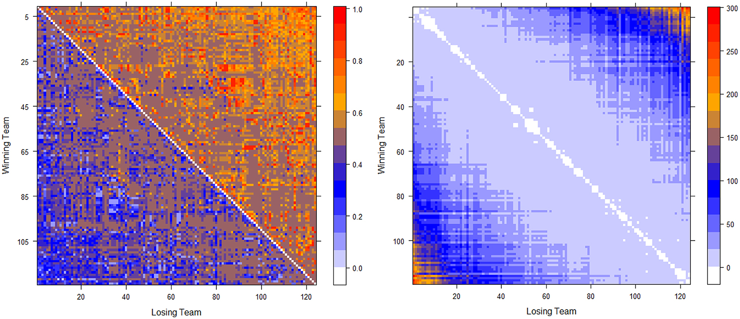
Figure 2. Optimally permuted ${\widehat{P}}_D({{W}}_0)$ (left panel) and Hamiltonian distance matrix with teams being arranged according to $\widehat{\sigma }*$ for the 2012 NCAA football season (right panel).

FIGURE 3

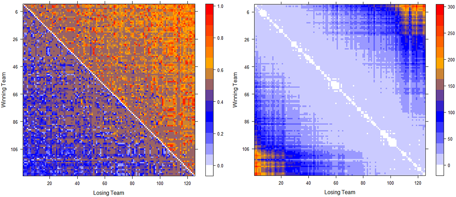
Figure 3. Optimally permuted ${\widehat{P}}_D({{W}}_0)$ (left panel) and Hamiltonian distance matrix with teams being arranged according to $\widehat{\sigma }*$ for the 2013 NCAA football season (right panel).

FIGURE 4

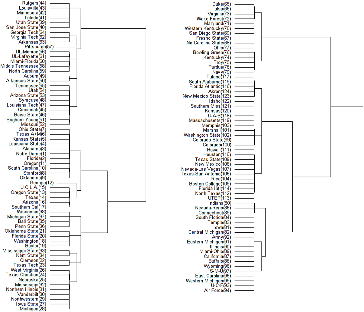
Figure 4. Hamiltonian distance based DCG tree for the 2012 NCAA football season. The tree has been cut at its highest level for ease of presentation. The branch containing the top 64 teams is displayed on left; the remaining teams are displayed on right. The number in the parentheses next to each team name is its position in $\widehat{\sigma }*$.

FIGURE 5

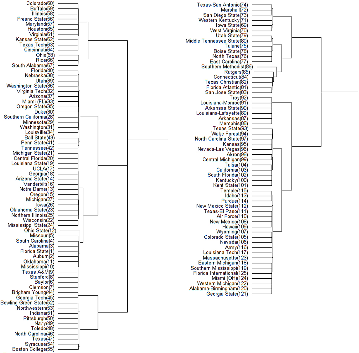
Figure 5. Hamiltonian distance based DCG tree for the 2013 NCAA football season. The tree has been cut at its highest level for ease of presentation. The branch containing the top 68 teams is displayed on left; the remaining teams are displayed on right. The number in the parentheses next to each team name is its position in $\widehat{\sigma }*$.

Next we address the task of extracting the power hierarchy embedded within ${\widehat{P}}_D({{W}}_0)$. Here we build this power hierarchy via Ultrametric tree geometry based on a Hamiltonian distance matrix. Here, the new “distance” between two nodes is defined as the Hamiltonian incurred by switching the two nodes' positions in ${\widehat{\sigma }}^{*}$ subtracting the minimum Hamiltonian ${H}(U({\widehat{\sigma }}^{*})\overline{D}({{W}}_0)U^T({\widehat{\sigma }}^{*}))$. Small values of such a distance indicate that these two nodes are indeed nearly equal in the power hierarchy, and should share a core cluster. By arranging the football teams on the new distance matrix according to ${\widehat{\sigma }}^{*}$, as shown right panels of in Figure 2 for Year 2012 and Figure 3 for year 2013, the presence of a serial of small white blocks along the diagonal is clearly visualized. This block pattern information confirms that the permutation resulting from the simulated annealing algorithm is reasonable. Each white block indeed indicates a core cluster, in which all involved teams are considered equal in power or dominance.

Further core clusters, which only include nodes being very close to each others, should be allowed to merge into a conglomerate cluster upon a higher level of hierarchy. By discovering all involved levels, an Ultrametric tree geometry is built (see [19, 20] for the detailed algorithmic construction) called Data Cloud Geometry (DCG). It is essential to point out here that such a distance has a built-in global ingredient, which is implicitly critical in constructing an Ultrametric tree geometry. The two Ultrametric tree geometries pertaining to two years of NCAA college football are shown in Figures 6, 7, respectively.

FIGURE 6

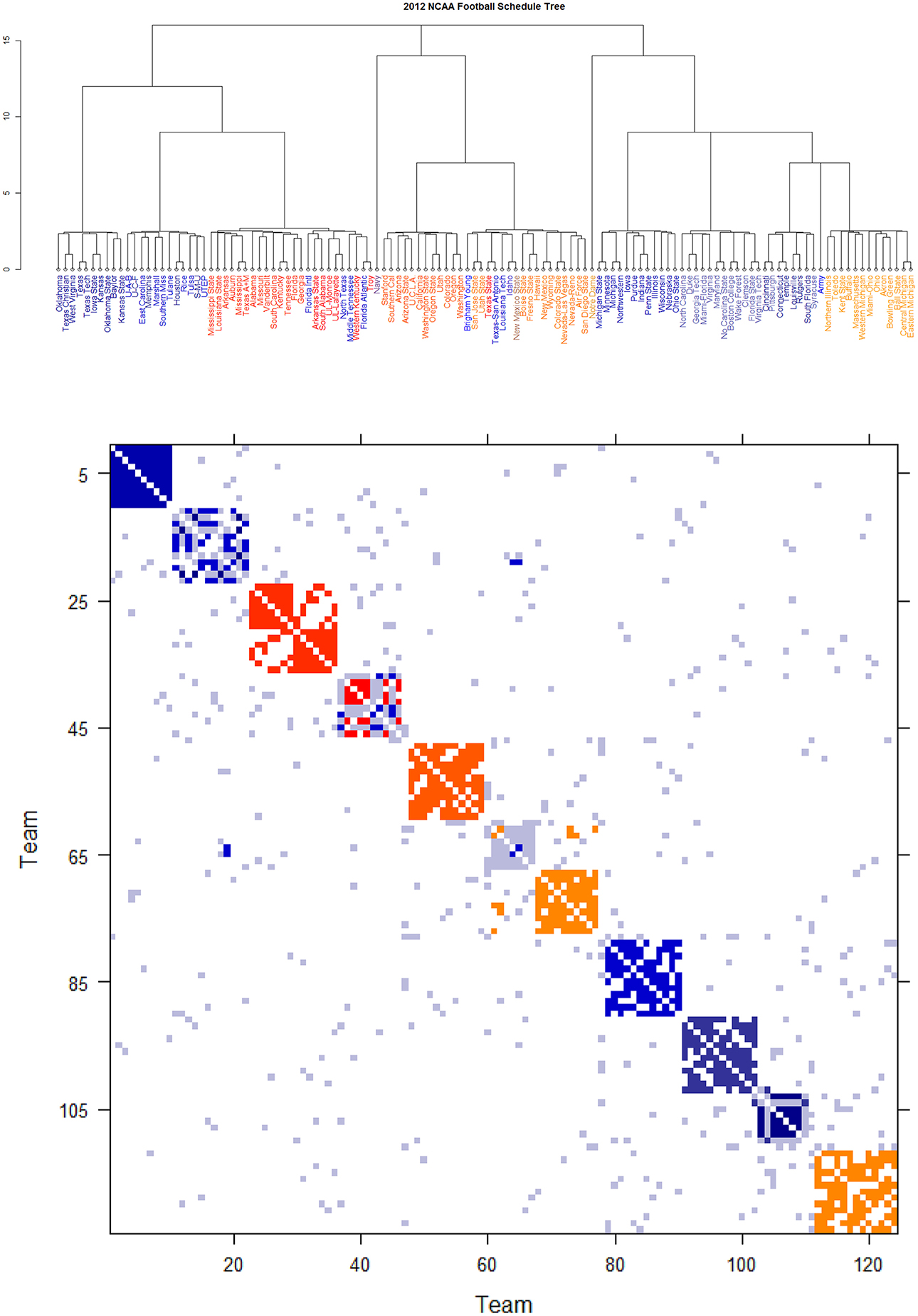
Figure 6. Schedule DCG tree and its induced schedule matrix ${S}$₀ of NCAA football data on year 2012: (Upper panel) DCG tree and (Lower panel) Parisi adjacency matrix with colored diagonal blocks marking the intra-conference games for the real conferences, and off-diagonal inter-conference games are marked in gray. The six independent teams are scatted on the tree. Conferences, from blue to red, are ACC, American, Big 12, Big Ten, Conference-USA, Independent schools, Mid-American, Mountain West, Pac 12, SEC, and Sun Belt.

FIGURE 7

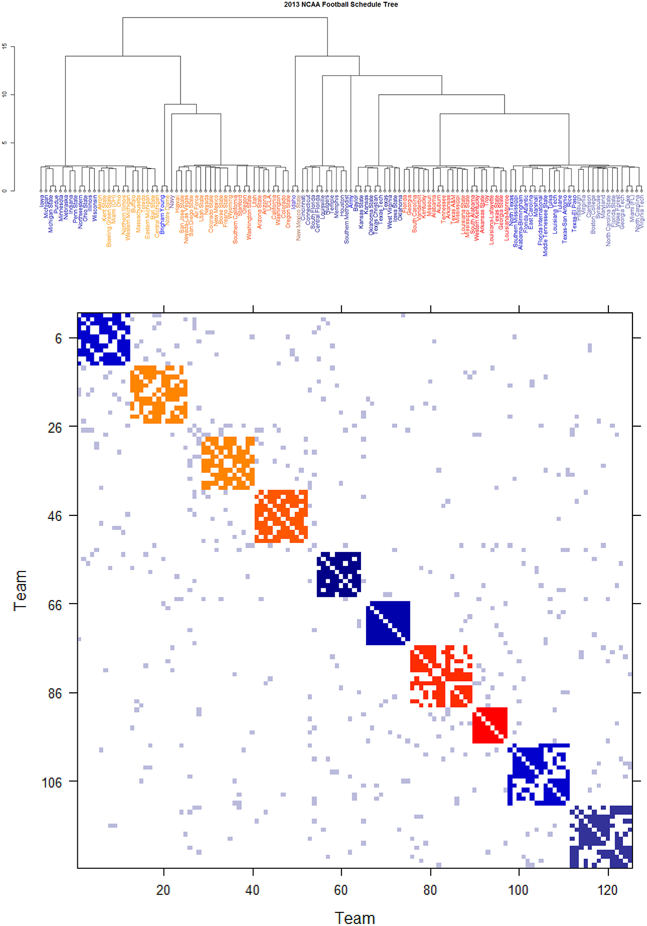
Figure 7. Schedule DCG tree and its induced schedule matrix ${S}$₀ of NCAA football data on year 2013: (Upper panel) DCG tree and (Lower panel) Parisi adjacency matrix with colored diagonal blocks marking the intra-conference games for the real conferences, and off-diagonal inter-conference games are marked in gray. The six independent teams are scatted on the tree. Conferences, from blue to red, are ACC, American, Big 12, Big Ten, Conference-USA, Independent schools, Mid-American, Mountain West, Pac 12, SEC, and Sun Belt.

3.1.1. Refined Version of Power Structural Hierarchy

The estimation of the m × m dominance probability matrix P_D(${W}$₀) via ${\widehat{P}}_D({{W}}_0)$ derived above can be improved by considering the following version of local transitivity. We propose to compute local transitivity between nodes i and j with ultrametric tree (level-based) distance d_ij as ${\widehat{T}}_{ij}={\widehat{T}}^{1∕d_{ij}}$. For instance, in Figures 6, 7, two teams sharing the same core cluster on the bottom tree level would have distance d_ij = 1, two team sin the same cluster on the second-lowest tree level would have distance d_ij = 2, and so on. We then update α₀ with a recalculated α_ij and re-run the Trickling percolation algorithm with a Beta Random field based on Beta random variables from Be(α_ij + 1, 1). The idea behind this is that Beta random variables from Be(α_ij + 1, 1) are closer to reality than Be(α₀ + 1, 1) in the sense that the simulated dominance paths are expected to be expanded and the number of unrealistic simulated “upset” games are significantly reduced. Then a refined version of $\overline{D}({{W}}_0)$ is computed, and a more efficient estimate ${\widehat{P}}_D({{W}}_0)$ is constructed. This improvement on estimating P_D(${W}$₀) turns out to be crucial because of the inherent sensitivity in mimicking directed binary networks as will be discussed in the next subsection.

3.2. Systemic Structures II: Randomness

From the NCAA Football competitive system, the observed directed binary network ${G}$(${W}$_′) is understood to have two sources of uncertainty: the schedule network ${G}$(${A}$₀) and the Binomial stochastic mechanism ideally governed by P_D(${W}$₀), which is responsible for transforming ${G}$(${A}$₀) into ${G}$(${W}$₀). We elaborate these sources briefly as follows.

The randomness embedded within a binary undirected network, ${A}$₀, has recently been studied in Fushing et al. [16]. It is now understood that such a component of randomness is constrained by its multiscale block patterns organized in the form of a Parisi adjacency matrix.

By taking ${G}$(${A}$₀) as a thermodynamic system equipped with Ising model potential, this Parisi adjacency matrix is computed as its minimum energy macrostate again by applying the DCG algorithmic computations, see Fushing et al. [16]. Its evident multiscale block patterns are explicitly revealed by superimposing the node organization pertaining to the computed DCG ultrametric tree onto rows and columns of the binary schedule matrix ${A}$₀.

The DCG ultrametric trees of the 2012 and 2013 NCAA college football schedules are computed and shown in Figures 6A, 7A, respectively. These Ultrametric trees rediscover the real conference structure of the college football teams. The three singletons are indeed independent teams: Notre Dame, Navy and Air Force. These tree also bring out which conferences are closer, and which are far apart. The resultant Parisi adjacency matrices with their multiscale block patterns are seen in Figures 2B, 3B. Such block information becomes evident when we compare Figure 1A with Figure 6B, as well as Figure 1B with Figure 7B. It is noted that the randomness pertaining to any block of ${G}$(${A}$₀) is the randomness of generating such a sub-matrix by subject to constraints of two sequences of row and column sums. Such an explicit use of randomness would be seen in the next section of Network mimicking.

The second source of randomness regarding to transforming ${G}$(${A}$₀) into ${G}$(${W}$₀) is pragmatically modeled via a Binomial stochastic mechanism on a game-by-game basis. We assume the global conditional independence given P_D(${W}$₀) among all football games. This assumption could be realistic under the setting of learning from the network data ${G}$(${W}$₀). In contrast, such an assumption of independence would be too simplistic when the data set is indeed a sequence of directed binary networks, which is realized along the series of football games sequentially played throughout the entire 13 week season.

3.3. Mimicking Directed Binary Networks and System's Robustness

Mimicking a directed binary network ${G}$(${W}$₀) is meant to generate a microscopic state, or microstate of the system as one whole. That is to say that any mimicry of directed binary network is required to conform to the computed deterministic structures, while its generating mechanism has to be carried out subject to the constraints pertaining to the identified randomness. An algorithm for mimicking a directed binary network is proposed below. A microstate ensemble can be derived by repeatedly applying this mimicking algorithm. We then make use of such a microstate ensemble to explore the systemic sensitivity, which is typically focused on a noticeable function of this system of interest. Here we designate the power ordering axis on the optimally permuted dominance probability matrix ${\widehat{P}}_D({{W}}_0$ as the “linear-like ranking function” from top to bottom. Such a linear-like ranking function is then evaluated on each member of the ensemble in the exact same way of computing ${\widehat{P}}_D({{W}}_0)$. The global variability along the whole spectrum of ranking ordering axis from Number one to Number m is evaluated in this sensitivity investigation.

3.3.1. Directed Binary Network Mimicking Algorithm

NB-1: Simulate a schedule matrix conforming to the finest block-patterns in its Parisi adjacency matrix of ${G}$(${A}$₀) (see [16] for this computational algorithm);

NB-2: Simulate win-and-loss matrix based upon the simulated schedule matrix and Binomial random mechanism with means being fixed corresponding to ${\widehat{P}}_D({{W}}_0)$.

By applying the above algorithm, a microstate ensemble of size 100 is generated for each of the two NCAA data on Years 2012 and 2013. Their linear-like ranking functions are evaluated and summarized in Tables 1, 2 below. We use the mimicked ranking standard deviation as an index of sensitivity of one team-node. The heterogeneity of sensitivity across the entire power ordering axis is clearly seen. In both tables, there is a noticeable increasing trend in standard deviation as teams become more lowly ranked; standard deviations then decrease again as approaching the most lowly-ranked teams. However, several outliers have significant large standard variations.

TABLE 1

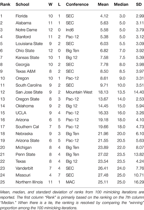
Table 1. Top 25 NCAA football teams for the 2012 season as ranked with respect to microstate ensemble.

TABLE 2

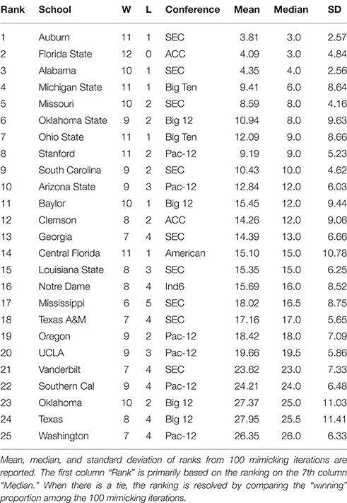
Table 2. Top 25 NCAA football teams for the 2013 season as ranked with respect to microstate ensemble.

In Table 1, we notice an outlier, San Jose State, with a significant large standard deviation with respect to its mimicked ranking median. San Jose State had a successful season, only losing two games. However, their conference (Mountain West) is generally considered to be one of the weaker conferences. Since San Jose State plays many of its games against teams in the Mountain West, we would expect them to win many of them. While San Jose State's standing within their conference is clear, it is much less apparent where they should be ranked among all teams. Here's a little bit more about San Jose State. It lost to Stanford (ranked 8th) and Utah State (ranked 39th). Our hypothesis is that the simulated annealing wanted to put them as high as possible, without surpassing Utah State. In fact, all 9 teams that San Jose State defeated are ranked below them, so with respect to only their own schedule, they are ranked appropriately at 40 in the computed ${\widehat{\sigma }}^{*}$. Why is it ranked 12th based on the microstate ensemble?

We also notice from their schedule that it played 4 independent teams. These games are necessarily played again in every simulated schedule, since each independent team is treated as its own conference. Since San Jose State won all 4 of these games, they will have a very good chance of winning those 4 games again in the mimicked seasons, since those games were actually played, the dominance probability is particularly high. However, it might not play with the Utah State in mimicked seasons. If they meet, then San Jose State could even win over Utah State with a positive probability. Due to such uncertainty in the mimicked schedule and in Beta random field adapted to ${\widehat{P}}_D({{W}}_0)$, San Jose State has a significant large variation in linear ranking. We see this inflation of standard deviation for top teams in weaker conferences (Northern Illinois in 2012 and Central Florida in 2013 have the same characteristic), and also for bottom-dwelling teams in strong conferences. This phenomenon to some extent nicely explains the sensitivity of this network mimicking.

We also see that the microstate ensemble does not always place undefeated teams at the top of the rankings. In Table 1, Notre Dame and Ohio State were both undefeated, but were ranked third and sixth, respectively. While we do not directly observe evidence for any other teams to be more highly ranked, we must accept that neither team is from the most dominant conference in 2012, the SEC. Neither team had many games played against other highly-ranked teams, while SEC teams such as Florida and Alabama had a higher level of competition. In 2013, the same phenomenon occurs with Florida State. Florida State's conference, the ACC, is broadly considered a weaker conference than the SEC. As a result, we are more hesitant to give Florida State the top ranking because their level of competition was lower than Auburn's, even though Auburn lost one game.

In summary, aforementioned episodes linking to the heterogeneity in ranking sensitivity clearly indicates that NCAA college football is a rather complex system of competition.

As a final note on our sensitivity exploration, beyond our mimicking algorithm, other simulated ensembles of ${G}$(${W}$₀) could be derived, for instance, by enlarging focal scales on the Parisi adjacency matrix on ${G}$(${A}$₀). With the NCAA data, this type of simulated ensemble corresponds to schedules swapping between different conferences. Our experimental results drastically vary from what are reported here in the Tables 1, 2 even when schedule swapping is only limited between nearest conferences. This sensitivity is likely due to the fact that the dyadic data in NCAA data is sparse. Consider a simulated game involving two teams in two different conferences. The two teams likely have few common opponents. Any upset loss resulted from such a simulated game would create a large amount of uncertainty when it comes to predicting the more dominant team. Even such a seemingly unremarkable simulated event may obscure the whole power structure.

4. Discussion

Our computational and algorithmic developments on directed binary networks show the capability of extracting deterministic structures and randomness of the underlying complex system of interest. The compositional constructs advance our systemic understanding in a critical way. The platform of network mimicking is proven to have impacts on exploring a system's functional sensitivity. By putting together all computed results from all considered perspectives, we should be able to advance further our understanding of a complex system.

Through the illustrating NCAA college football example, we clearly see complexity embedded within this competitive system, while at the same time we are able to recognize realistically the complicated information contents contained in a seemingly simplistic directed binary network. This fact reminds us that understanding a system of scientific interest does require a heavy investment on computing.

At this stage there are still many key technical difficulties remaining unsolved. They are tentatively resolved with heuristic approaches or proposals in this paper. Some questions that particularly need rigorous endeavors are listed as follows: How can we effectively measure and estimate pairwise transitivity T_ij and the related parameter α_ij? How much confidence can be placed on the blank entries of ${\widehat{P}}_D({{W}}_0)$?

Here it is worth emphasizing again the network mimicking principle: any mimicked network must be taken as a microscopic state that is generated coherently with respect to the system's randomness, and conforms to the system's deterministic structures.

The proposed directed binary network mimicking algorithm would allow us to evaluate the network entropy. This entropy should be the sum of the entropy pertaining to the finest scale block patterns of the Parisi adjacency matrix (which is computed by measuring the sizes of corresponding microstate ensembles as discussed in [16]), plus the entropy derived from the Binomial random mechanism with means being fixed corresponding to ${\widehat{P}}_D({{W}}_0)$.

On the other hand. this NCAA football analysis comes at a particularly opportune time, as the NCAA recently changed the postseason format from a single championship game to a four-team playoff. The teams participating in the playoff will be decided by an appointed committee, rather than by a computer and/or voting system like the Bowl Championship Series (BCS). A linear-like ranking hierarchy such as the one developed in this paper could be applied to provide the committee with some objectivity in choosing the participating schools, or even the number of schools that are to participate. Trees such as those in Figures 4, 5 can be used to determine the contents of the highest tier of football teams, while rankings derived based on the microstate ensemble, holding conferences constant, provide insight into the level of uncertainty we might have about teams' relative standing.

As a final remark, we mention one implication of our sensitivity explorations on the power hierarchy of NCAA Football League. These investigations clearly show the difficulties in pertinent and realistic network modeling and its statistical inferences. At this stage there is no available methodology or even knowledge for how to physically generate multiscale block-patterns without knowing the tree structure priori, neither for the power structural hierarchy. The unavailability is not surprising because that a network is better perceived as a complex system itself. The network mimicking principle proposed here might serve as a guide on network modeling, goodness-of-fit testing and making inferences.

Author Contributions

FH and KF designed the experiments and analyzed data. FH did most writing and KF performed all computing.

Conflict of Interest Statement

The authors declare that the research was conducted in the absence of any commercial or financial relationships that could be construed as a potential conflict of interest.

Acknowledgments

This research is supported in part by the NSF under Grants No: DMS 1007219 [co-funded by Cyber-enabled Discovery and Innovation (CDI) program].

References

1. Crutchfield JP. Between order and chaos. Nat Phys. (2012) 8:17–24. doi: 10.1038/nphys2190

PubMed Abstract | CrossRef Full Text | Google Scholar

2. Simon HA. The architecture of complexity. Proc Am Philos Soc. (1962) 106:467–82.

Google Scholar

3. Anderson PW. More is different. Science (1972) 177:393–6. doi: 10.1126/science.177.4047.393

PubMed Abstract | CrossRef Full Text | Google Scholar

4. Crutchfield JP, Machta J. Introduction to focus issue on “randomness, structure, and causality: measure of complexity from theory to applications. Chaos (2011) 21:037101.

Google Scholar

5. Albert R, Barabási AL. Statistical mechanics of complex network. Rev Mod Phys. (2002) 74:47–97.

Google Scholar

6. Barzel B, Barabási AL. Universality in network dynamics. Nat Phys. (2013) 9:673–81.

PubMed Abstract | Google Scholar

7. Gao J, Barzel B, Barabási AL. Universal resilience patterns in complex networks. Nature (2016) 530:307–12. doi: 10.1038/nature18019

PubMed Abstract | CrossRef Full Text | Google Scholar

8. Doyle JC, Csete M. Architecture, constraints and behavior. Proc Natl Acad Sci USA (2011) 108:15624–30. doi: 10.1073/pnas.1103557108

PubMed Abstract | CrossRef Full Text | Google Scholar

9. Fujii K, Fushing H, Beisner B, McCowan B. Computing Power Structures in Directed Biosocial Networks: Flow Percolation and Imputed Conductance. Technical Report. Department of Statistics, UC Davis, Davis (2016).

10. Landau HG. On dominance relations and the structure of animal societies. I. effect of inherent characters. Bull Math Biophys. (1951) 13:1–19. doi: 10.1007/BF02478336

CrossRef Full Text | Google Scholar

11. Kendall MG. Rank Correlation Methods. London: Charles Griffin (1962).

Google Scholar

12. Appleby MC. The probability of linearity in hierarchies. Anim Behav. (1983) 31:600–8. doi: 10.1016/S0003-3472(83)80084-0

CrossRef Full Text | Google Scholar

13. Kasuya E. A randomization test for linearity of dominance hierarchies. J Ethol. (1995) 13:137–40. doi: 10.1007/BF02352574

CrossRef Full Text | Google Scholar

14. de Vries H. Finding a dominance order most consistent with a linear hierarchy: a new procedure and review. Anim Behav. (1998) 55:827–43. doi: 10.1006/anbe.1997.0708

PubMed Abstract | CrossRef Full Text | Google Scholar

15. Leicht EA, Newman MEJ. Community structure in directed networks. Phys Rev Lett. (2008) 100:118703. doi: 10.1103/PhysRevLett.100.118703

PubMed Abstract | CrossRef Full Text | Google Scholar

16. Fushing H, Chen C, Liu S, Koehl P. Bootstrapping on undirected binary networks via statistical mechanics. J Stat Phys. (2014) 156:823–42. doi: 10.1007/s10955-014-1043-6

PubMed Abstract | CrossRef Full Text | Google Scholar

17. Fushing H, McAssey MP, McCowan B. Computing a ranking network with confidence bounds from a graph-based Beta random field. Proc R Soc A (2011) 467:3590–612. doi: 10.1098/rspa.2011.0268

PubMed Abstract | CrossRef Full Text | Google Scholar

18. Kirkpatrick S, Gelatt CD, Vecchi MP. Optimization by simulated annealing. Science (1983) 220:671–80. doi: 10.1126/science.220.4598.671

PubMed Abstract | CrossRef Full Text | Google Scholar

19. Fushing H, McAssey MP. Time, temperature and data cloud geometry. Phys Rev E (2010) 82:061110. doi: 10.1103/PhysRevE.82.061110

PubMed Abstract | CrossRef Full Text | Google Scholar

20. Fushing H, Wang H, Van der Waal K, McCowan B, Koehl P. Multi-scale clustering by buildi ng a robust and self-correcting ultrametric topology on data points. PLOS ONE (2013) 8:e56259. doi: 10.1371/journal.pone.0056259

PubMed Abstract | CrossRef Full Text