Piecewise-Linear Maps and Their Application to Financial Markets

1. Introduction

Two of the most important characteristics of the dynamics of financial markets are that asset prices may substantially disconnect from their fundamental values and that asset prices are excessively volatile. Without question, these phenomena may be quite harmful for the real economy, as witnessed, for instance, by the Great Depression, triggered by the world-wide stock market crash in 1929, and the Great Recession, triggered by the world-wild stock market crash in 2007 (see e.g., [1–3]). However, three further statistical properties of asset price dynamics have received increasing attention in the finance literature. First, asset prices are—despite their boom-bust behavior—hardly predictable and their time evolution thus closely resembles a random walk. Second, the distribution of returns, i.e., the distribution of relative (or log) asset price changes, displays fat tails, meaning, in particular, that extreme price fluctuations emerge more frequently than warranted by the normal distribution. Third, volatility tends to cluster in the sense that periods of low volatility alternate with periods of high volatility. Surveys of the stylized facts of financial markets are provided, among others, by Mantegna [4], Cont [5], and Lux and Ausloos [6].

Agent-based financial market models seek to explain these challenging phenomena. For general reviews of this research field see, for instance [7–9]. Supported by experimental evidence [10] and questionnaire studies [11], these models assume that financial market participants rely on technical and fundamental trading rules to determine their orders. Technical analysis [12] aims at identifying trading signals out of past price movements and suggests buying (selling) when asset prices increase (decrease). In contrast, fundamental analysis [13] is based on the belief that asset prices return toward their fundamental values and thus suggests buying (selling) in undervalued (overvalued) markets. Agent-based models by e.g., Day et al. [14], De Grauwe et al. [15], Lux [16], Brock and Hommes [17], Farmer and Joshi [18], Chiarella et al. [19], and Franke and Westerhoff [20] show that interactions between traders relying on technical and fundamental analysis rules can generate complex price dynamics. Within the seminal model of Day et al. [14], for instance, destabilizing traders dominate the market near fundamental values and initiate bull or bear markets. Far from fundamental values, however, stabilizing fundamental traders become increasingly active and drive asset prices back to fundamental values. Since the relative strength of technical and fundamental trades thus constantly changes, the model produces intricate price fluctuations.

The goal of our paper is to review agent-based financial market models in which the dynamics is driven by piecewise-linear maps. Examples from this stream of literature include, for instance [21–25]. One important advantage of piecewise-linear maps is that they allow very clear analytical insights into the functioning of the underlying model. Another interesting aspect of such maps is that they give rise to very puzzling dynamics. For instance, the transition between fixed point dynamics and chaotic motion can be very abrupt, i.e., a tiny change in one of the model's parameters can have a significant effect on the model's dynamics. From a policy perspective, this is an important message since also small changes in policy measures can have great effects for the stability of financial markets. Piecewise-linear maps are naturally appealing to explain the dynamics of financial markets since abrupt regime changes may give rise to extreme price changes (thereby generating fat-tailed return distributions) and since infrequent changes between coexisting regimes may give rise to alternating periods of low and high volatility (thereby producing volatility clustering). Moreover, deterministic models have so far offered several novel reasons for the emergence of bull and bear markets and can also explain the excess volatility of asset prices. However, there are also a few stochastic models which mimic the stylized facts of financial markets quite well. Unfortunately, piecewise-linear models are still not completely understood. Working in this area may thus have the additional benefit that one discovers new dynamic phenomena such a new bifurcation structures. For a true scientist, that's of course quite exciting. By surveying the origins and some recent advances in this field we hope to motivate other researchers to start also working in this prospering research direction.

The remainder of our paper is organized as follows. In Section 2, we introduce the class of maps we use to study the dynamics of financial markets. In Section 3, we review the seminal model of Huang and Day [21]. In Section 4, we present two more recent lines of research. In Section 4.1, we first discuss models in which the trading behavior of the traders is more general than in Huang and Day [21]. In Section 4.2, we then report models in which the traders update their perception of the fundamental value over time. Finally, Section 5 concludes our paper.

2. Piecewise-Linear Maps

A piecewise-linear, one-dimensional, map f(x) is characterized by at least two different definitions for different values of the dynamic variable x, that is:

$\begin{array}{cc}f(x)=\{\begin{array}{lll}{f}_1(x)\hfill & \text{for }\hfill & x\in D_1\hfill \\ f_2(x)\hfill & \text{for }\hfill & x\in D_2\hfill \\ \mathrm{..}\hfill & \hfill & \hfill \\ f_n(x)\hfill & \text{for }\hfill & x\in D_n\hfill \end{array}& \left(1\right)\end{array}$

where:

•  n ∈ ℕ, n ≥ 2;

•  f_k(x) with k = 1, .., n are all linear/affine functions;

• D_k with k = 1, .., n are non-overlapping intervals of real numbers. To each bounding value x = x_k separating D_k from D_k+1, it can be applied either f_k(x) or f_k+1(x), not both;

• D₁ and D_n can be unbounded.

In Figure 1 we have represented a linear function (Figure 1A), a piecewise-linear continuous function defined differently in two contiguous intervals (Figure 1B), a piecewise-linear discontinuous function defined differently in two contiguous intervals (Figure 1C) a finally a piecewise-linear discontinuous function defined differently in three contiguous intervals with two discontinuity points (Figure 1D).

FIGURE 1

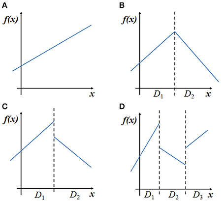
Figure 1. In (A) a linear map. In (B) a piecewise-linear continuous map with two regimes. In (C) a piecewise-linear discontinuous map with two regimes. In (D) a piecewise-linear discontinuous map with three regimes.

Basically, the main feature of piecewise smooth (continuous or not) systems is that there is a change of definition when a border separating D_i and D_i+1 is crossed or met¹. This gives rise to a peculiar kind of bifurcation, nowadays known as border collision bifurcations (BCBs henceforth), and firstly introduced by Nusse and Yorke [26, 27] and Maistrenko et al. [28–30]². BCBs cause the passage from one attractor to another like other local bifurcation of smooth functions, but in this case the transition can be abrupt. By changing the value of a parameter, a point of the attractor can collide with the border of the region of definition and after that a new attractor appears. It is possible to pass from a cycle to chaos (or the opposite) without following the well-known “routes to chaos” typical of smooth functions. Even in the one-dimensional linear version (1), which is the simplest, all the features of these maps have still not been completely understood. A lot of work has been done on one-dimensional piecewise-linear maps with only one not derivability (or discontinuity) point (i.e., two regimes maps, surveyed in Avrutin et al. [35]) and some work on maps with three linear pieces or two-dimensional maps.

Piecewise smooth systems are relevant in many applications, from Electrical and Mechanical Engineering ([28, 29, 36–40], among the others) to Sociology (see [41, 42]), but one of the main fields of application is Economics. We mention here Business Cycle models (see [43, 44]), Growth models [45] and Oligopoly models [46, 47]. In the next sections of the paper we illustrate their application to financial markets, starting from the seminal paper of Huang and Day [21].

3. The Huang-Day (1993) Model

Huang and Day (1993) propose a simple prototype financial market model with a market maker and two types of traders. The two trader types differ in their reaction to the markets misalignment, i.e., the difference between the asset price and its fundamental value, and are called fundamentalists and chartists³.

Fundamentalists buy the asset when it is undervalued (that is the price is lower than its fundamental value) and sell it when it is overvalued (that is the price is higher than the fundamental value). Their excess demand is formalized as follows:

$\begin{array}{cc}{D}_t^F=\{\begin{array}{lll}A\hfill & \text{if}\hfill & P_t<Z^{F,B}\hfill \\ f(Z^{F,D}-P_t)\hfill & \text{if}\hfill & Z^{F,B}\le P_t<Z^{F,D}\hfill \\ 0\hfill & \text{if}\hfill & Z^{F,D}\le P_t<Z^{F,U}\hfill \\ -f(P_t-Z^{F,U})\hfill & \text{if}\hfill & Z^{F,U}\le P_t<Z^{F,T}\hfill \\ -A\hfill & \text{if}\hfill & Z^{F,T}\ge P_t\hfill \end{array}& \left(2\right)\end{array}$

where P is the asset price, A > 0 is a fixed amount of assets, f > 0 measures the strength of the response of the investors to the misalignment and the other parameters are threshold prices, such that:

$Z^{F,B}<Z^{F,D}<F<Z^{F,U}<Z^{F,T}$

where F is the exogenously given fundamental value.

The interpretation of the excess demand (Equation 2) is the following. When the price is close to its fundamental value, i.e., between Z^F,D and Z^F,U, these traders think that the chance of gain or loss is basically zero and they do not move their portfolios. When the price crosses the upper or the lower sensitivity thresholds (Z^F,D and Z^F,U) they start to buy or sell the asset and the amount is proportional to the distance between the price and the crosses threshold and also proportional to the reaction parameter f. Finally, there are two extreme thresholds, Z^F,B and Z^F,T, that, if crossed by the price, permit to this kind of traders to conclude that the price is going to go back toward its fundamental value almost certainly, so they buy or sell a fixed amount A ≡ f(Z^F,T − Z^F,U) = f(Z^F,D − Z^F,B).

Chartists are assumed to be optimistic when the price is higher than the fundamental value and pessimistic in the opposite case, so they will buy the asset in the first case and sell it in the second one. Their excess demand is the following:

$\begin{array}{cc}{D}_t^C=c(P_t-F)& \left(3\right)\end{array}$

where c is a positive reaction parameter.

Finally, as usual in this branch of the literature, there is a market maker who adjusts the asset price from period to period according to the total excess demand:

$\begin{array}{cc}{P}_{t+1}=P_t+a(D_t^F+D_t^C)& \left(4\right)\end{array}$

By substituting the excess demands (Equations 2, 3) into the market maker (Equation 4) we get the following one-dimensional piecewise-linear map regulating price movements:

$\begin{array}{cc}{P}_{t+1}=\{\begin{array}{lll}{f}_1(P_t)=k_1+\pi P_t\hfill & \text{if}\hfill & P_t<Z^{F,B}\hfill \\ f_2(P_t)=k_2+\rho P_t\hfill & \text{if}\hfill & Z^{F,B}\le P_t<Z^{F,D}\hfill \\ f_3(P_t)=k_3+\pi P_t\hfill & \text{if}\hfill & Z^{F,D}\le P_t<Z^{F,U}\hfill \\ f_4(P_t)=k_4+\rho P_t\hfill & \text{if}\hfill & Z^{F,U}\le P_t<Z^{F,T}\hfill \\ f_5(P_t)=k_5+\pi P_t\hfill & \text{if}\hfill & Z^{F,T}\ge P_t\hfill \end{array}& \left(5\right)\end{array}$

where:

$\begin{array}{l}\pi =1+ac\hfill \\ \rho =1-a(f-c)\hfill \\ k_1=a(A-cF)\hfill \\ k_2=a(f{Z}^{F,D}-cF)\hfill \\ k_3=-acF\hfill \\ k_4=-a(f{Z}^{F,U}+cF)\hfill \\ k_5=-a(A+cF)\hfill \end{array}$

The piecewise-linear map (Equation 5), whose typical shape is represented in Figure 2A, permits Huang and Day to obtain price movements such as those represented in Figure 2B, that endogenously generate bull and bear fluctuations through the emergence of chaotic dynamics with regime switching, so these dynamic are at the same time bounded but also almost unpredictable. The bifurcation diagrams in Figure 3 do not only show how high values of the chartists' reaction parameter and/or low values of the fundamentalists' reaction parameter may generate complex dynamics, but also show a peculiarity of piecewise defined maps: the sudden transition by varying some parameters, from convergence to a steady state to complex dynamics, without the gradualness of the routes to chaos typical of smooth functions.

FIGURE 2

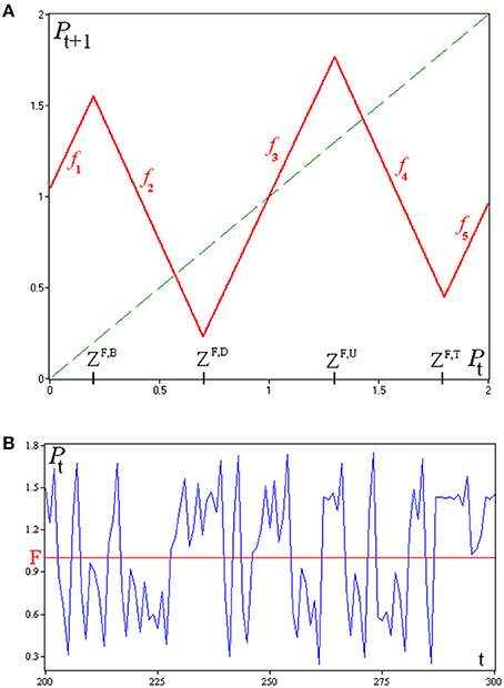
Figure 2. The shape of the map (A) and a timeplot (B) obtained by using the following set of parameters: a = 2.6, c = 0.6, f = 2, F = 1, Z^F,B = 0.2, Z^F,D = 0.7, Z^F,U = 1.3, Z^F,T = 1.8.

FIGURE 3

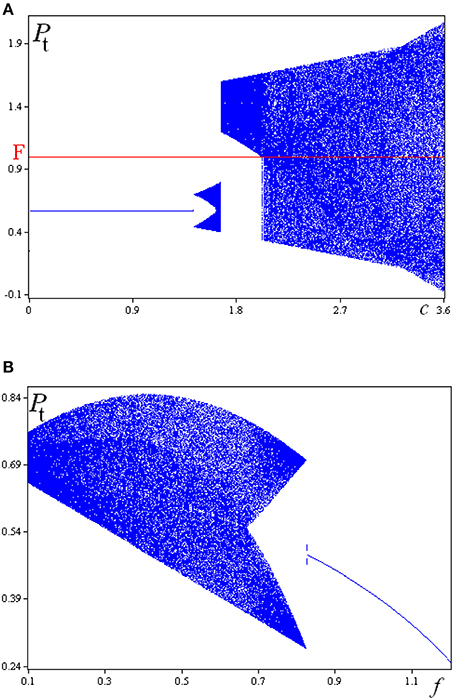
Figure 3. The bifurcation diagram with respect to c (A) is obtained by using a = 1.7, while the bifurcation diagram with respect to f (B) is obtained with a = 2.6. The remaining parameters are the same used in Figure 2.

Day [48] extends this model by considering different types of fundamentalists and different types of chartists. For instance, by assuming three types of fundamentalists and one type of chartists he obtains a one-dimensional piecewise-linear map made up by eleven linear pieces. In this way he can replicate even better some stylized facts of financial markets such as ascending and descending triangles, wedges, breakways, runaways and exhaustion price patterns—typical price formations observed by technical traders in real markets [12].

4. Recent Generalizations and Extensions

Piecewise defined maps permit, as we have seen, to model price movements that depend upon different regimes. The switches among the various regimes and the occurring of the so-called border-collision bifurcations, make unnecessary to introduce nonlinear functions (for instance, in the market maker mechanism or in some behavioral rule) in order to obtain complicated price and qualitatively realistic price movements.

More recently some researchers have tried to explain by using piecewise defined maps some stylized facts of financial market, not only qualitatively but also quantitatively. In this section we refer to two of these new strands of research. The first one is a generalization of the Huang and Day [21] paper and is a deterministic model used also as a basis for the introduction of some stochastic elements. The second model we consider extends to its extreme consequences the potentiality of piecewise-linear maps, by considering an high (potentially infinite) number of regimes and discontinuity points.

4.1. A Mixed Deterministic/Stochastic Piecewise Linear Model

In a series of papers, [24, 25, 49–52] extend the framework of Huang and Day [21] in the following sense:

• they consider threshold values of the misalignment also for chartists;

• they consider that the fixed amounts of the assets the traders may buy or sell in the different regimes do not necessarily depend on the thresholds;

• they introduce the possibility for an asymmetric behavior of the traders in bull and bear markets.

From a mathematical point of view, the map they build is not only one-dimensional and piecewise-linear (as in the original model of Huang and Day), but also in general discontinuous. While equilibria may not exist, erratic endogenous switching among the various regimes may arise, mimicking some important stylized facts of financial markets. However, under some suitable parameter values, they can recover the one-dimensional piecewise-linear and continuous model of Huang and Day as a special case.

To be precise, they consider a market maker who adjusts the log price of the asset on the basis of a log-linear price adjustment rule:

$\begin{array}{cc}{P}_{t+1}=P_t+a\left(D_t^{C,1}+D_t^{F,1}+D_t^{C,2}+D_t^{F,2}\right)& \left(6\right)\end{array}$

where the four excess demand terms in bracket characterize the trading rule of four groups of speculators (two types of fundamentalists and two types of chartists).

Let us start by considering the first type of chartists. Their transactions are given by the following rule:

$\begin{array}{cc}{D}_t^{C,1}=\{\begin{array}{lll}{c}^{1,a}+c^{1,b}(P_t-F)\hfill & \text{for}\hfill & P_t-F\ge 0\hfill \\ -c^{1,c}+c^{1,d}(P_t-F)\hfill & \text{for}\hfill & P_t-F<0\hfill \end{array}& \left(7\right)\end{array}$

where the parameters are all non-negative and in particular c^1,b and c^1,d are reaction parameters, while c^1,a and c^1,c denote the amount of the asset they buy (resp. sell) in the bull (resp. bear) market, that do not depend on the size of the misalignment.

So, with respect to the chartists considered by Huang and Day [21] they may have different reactivities in the two regimes and their order only partially depend upon how much the current price deviates from its fundamental value.

The first type of fundamentalists behaves as follows:

$\begin{array}{cc}{D}_t^{F,1}=\{\begin{array}{lll}-f^{1,a}+f^{1,b}(F-P_t)\hfill & \text{for}\hfill & P_t-F\ge 0\hfill \\ f^{1,c}+f^{1,d}(F-P_t)\hfill & \text{for}\hfill & P_t-F<0\hfill \end{array}& \left(8\right)\end{array}$

where the non-negative parameters f^1,b and f^1,d are the reaction parameters for the bull and the bear market and f^1,a and f^1,c are non-negative too, characterizing the fixed amounts of assets they sell (resp. buy) in the bull and in the bear market.

This type of fundamentalist is different with respect to the fundamentalists of Huang and Day [21] not only for their potentially asymmetric behavior but also because they are always active, for any size of the distance between the price and the fundamental value.

The second type of trader (both chartists and fundamentalists) have the additional feature to remain inactive if the distance between the price and fundamental is not considered large enough to create an opportunity for making profits. Moreover, the thresholds can be different in the bull and in the bear market and those used by chartists can deviate from those adopted by fundamentalists.

Under these assumptions, the excess demand of type 2 chartists is:

$\begin{array}{cc}{D}_t^{C,2}=\{\begin{array}{lll}{c}^{2,a}+c^{2,b}(P_t-F)\hfill & \text{for}\hfill & P_t-F\ge Z^{C,U}\hfill \\ 0\hfill & \text{for}\hfill & -Z^{C,D}<P_t-F<Z^{C,U}\hfill \\ -c^{2,c}+c^{2,d}(P_t-F)\hfill & \text{for}\hfill & P_t-F\le -Z^{C,D}\hfill \end{array}& \left(9\right)\end{array}$

where the interpretation of the non-negative parameters c^2,a, c^2,b, c^2,c and c^2,d is the same already seen for type 1 chartists, with the additional restriction that:

$\begin{array}{ccc}{c}^{2,a}\ge -c^{2,b}\left(Z^{C,U}-F\right)& \text{and}& c^{2,c}\ge -c^{2,d}\left(Z^{C,D}+F\right)\end{array}$

that permit to avoid negative transactions in the bull market or positive transactions in the bear market. Z^C,U and −Z^C,D are the potentially different thresholds for becoming active in the bull and the bear market, respectively. The asymmetry between bull and bear markets and the possible inactivity differentiate these type of chartists from those considered by Huang and Day [21].

Finally, type 2 fundamentalists adopt the following trading rule:

$\begin{array}{cc}{D}_t^{F,2}=\{\begin{array}{lll}-f^{2,a}+f^{2,b}(F-P_t)\hfill & \text{for}\hfill & P_t-F\ge Z^{F,U}\hfill \\ 0\hfill & \text{for}\hfill & -Z^{F,D}<P_t-F<Z^{F,U}\hfill \\ f^{2,c}+f^{2,d}(F-P_t)\hfill & \text{for}\hfill & P_t-F\le -Z^{F,D}\hfill \end{array}& \left(10\right)\end{array}$

with non-negative parameters. Also in this case the following restrictions must hold:

$\begin{array}{ccc}{f}^{2,a}\ge f^{2,b}\left(F-Z^{F,U}\right)& \text{and}& f^{2,c}\ge f^{2,d}\left(Z^{,D}+F\right)\end{array}$

in order to have non-negative order in the bear market and non-positive order in the bull market.

The asymmetry between bull and bear markets would make this type of fundamentalists different from those considered by Huang and Day [21].

Now that the four excess demands have been specified we can build the model's law of motion. The authors always use the simplifying restriction:

$z=Z^{C,U}=Z^{C,D}=Z^{F,U}=Z^{F,D}$

that permits to obtain a four pieces map, expressed in deviation from the fundamental value ($\tilde{P}=P-F$):

$\begin{array}{cc}{\tilde{P}}_{t+1}=\{\begin{array}{lll}{m}^1+m^3+(1+s^1+s^3){\tilde{P}}_t\hfill & \text{for}\hfill & {\tilde{P}}_t\ge z\hfill \\ m^1+(1+s^1){\tilde{P}}_t\hfill & \text{for}\hfill & 0\le {\tilde{P}}_t<z\hfill \\ m^2+(1+s^2){\tilde{P}}_t\hfill & \text{for}\hfill & -z<{\tilde{P}}_t<0\hfill \\ m^2+m^4+(1+s^2+s^4){\tilde{P}}_t\hfill & \text{for}\hfill & {\tilde{P}}_t\le -z\hfill \end{array}& \left(11\right)\end{array}$

where the parameters have been grouped as follows:

$\begin{array}{cc}{m}^1=c^{1,a}-f^{1,a},& s^1=c^{1,b}-f^{1,b},\\ m^2=f^{1,c}-c^{1,c},& s^2=c^{1,d}-f^{1,d},\\ m^3=c^{2,a}-f^{2,a},& s^3=c^{2,b}-f^{2,b},\\ m^4=f^{2,c}-c^{2,c},& s^4=c^{2,d}-f^{2,d}.\end{array}$

Slopes and offsets of the piecewise-linear map (Equation 11) can be both positive and negative, giving rise to several quite different scenarios.

The authors have studied different subcases of the map (Equation 11). They have until now considered subcases with two branches and others with three branches. They obtain bull and bear dynamics due to the chaotic motion of prices.

These models are surveyed in Tramontana and Westerhoff [53] where they also consider a stochastic version with calibrated parameters. They move from a version of the map (Equation 11) where m¹ = m² and s¹ = s². In this way they obtain a three pieces piecewise-linear and in general discontinuous map that forms the deterministic skeleton of their model:

$\begin{array}{cc}{\tilde{P}}_{t+1}=\{\begin{array}{lll}{m}^1+m^3+(1+s^1+s^3){\tilde{P}}_t\hfill & \text{for}\hfill & {\tilde{P}}_t\ge z\hfill \\ m^1+(1+s^1){\tilde{P}}_t\hfill & \text{for}\hfill & -z<{\tilde{P}}_t<z\hfill \\ m^1+m^4+(1+s^1+s^4){\tilde{P}}_t\hfill & \text{for}\hfill & {\tilde{P}}_t\le -z\hfill \end{array}& \left(12\right)\end{array}$

Then, they fix the fundamental value to F = 0 and the symmetric threshold to z = 0.2 and calibrate, with a trial and error calibration process, the other six parameters, assumed to be normally distributed. The shape of the deterministic skeleton of the model is represented in Figure 4 where the three linear pieces and the two discontinuity points are clearly visible. The bifurcation diagrams in Figure 5 are an example of the kind of complex scenarios that may arise from such a map.

FIGURE 4

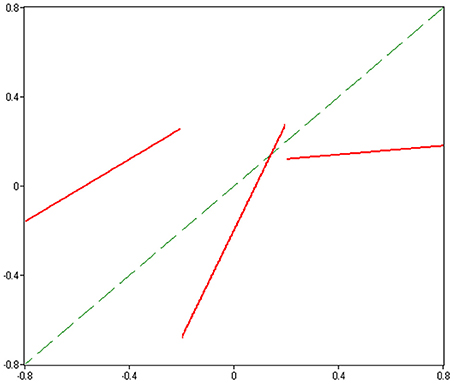
Figure 4. The shape of the map is obtained by using m¹ = −0.2, m³ = 0.3, m⁴ = 0.6, s¹ = 1.4, s³ = −2.3, s⁴ = −1.7, and z = 0.2.

FIGURE 5

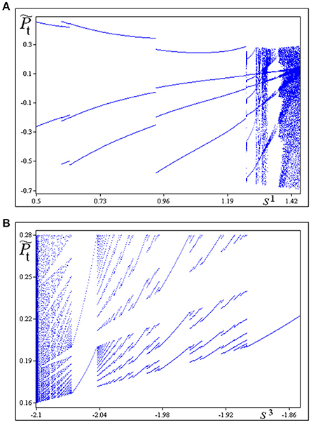
Figure 5. In (A) bifurcation diagram with respect to s¹, while in (B) with respect to s³. The other parameters are the same used for Figure 4.

By performing Monte Carlo simulations the authors replicate stylized facts of financial markets that are quite hard to obtain with a purely deterministic model. For instance, the simulation run depicted in Figure 6 reveals that the model is able to produce bubbles and crashes, excess volatility, fat tails for the distribution of the returns, uncorrelated returns and volatility clustering; typical phenomena observed in many financial markets. For a review of the stylized facts of financial markets see, for instance [5].

FIGURE 6

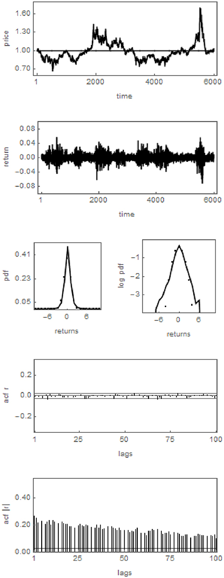
Figure 6. The panels show from top to bottom the evolution of prices, the corresponding returns, the distribution of returns (left panel: usual representation; right panel: log-linear representation), the autocorrelation function of returns and the autocorrelation function of absolute returns, respectively.

4.2. Increasing the Number of Branches

Weihong Huang, one of the two coauthors of the seminal work we moved from, and other collaborators have recently introduced a piecewise-linear framework to replicate the different kinds of crisis that may occur in financial markets. In particular they refer to the so-called sudden, disturbing and smooth crisis⁴. Examples of this line of work include, among others [22] and [23].

They consider a classic market maker mechanism with price movements regulated by the excess demand of chartists fundamentalists:

$\begin{array}{cc}{P}_{t+1}=P_t+a\left(D_t^C+D_t^F\right)& \left(13\right)\end{array}$

The excess demand of fundamentalists is linear and depends upon the difference between the actual price and an exogenously given fundamental value:

$\begin{array}{cc}{D}_t^F=f(F-P_t)& \left(14\right)\end{array}$

where f > 0 is a measure of the reactivity of fundamentalists.

The originality of this model relies on the chartists' trading rule. They are assumed to make a short-term expectation (P^β) for the asset value. Chartists subdivide the price domain into n regimes:

$r_1:\left[{\overline{P}}_0,{\overline{P}}_1\right],r_2:\left[{\overline{P}}_1,{\overline{P}}_2\right],\mathrm{\dots },r_n:\left[{\overline{P}}_{n-1},{\overline{P}}_n\right]$

and the short-term expectation varies according to the regime where the current asset price is located. In particular, the middle value of each regime represents the short-term expectation:

$\begin{array}{cc}{P}^{\beta }=\frac{{\overline{P}}_{j-1}+{\overline{P}}_j}{2}\text{ for }P\in r_j,j=1,2,\mathrm{\dots },n& \left(15\right)\end{array}$

and the trading rule of chartists is:

$\begin{array}{cc}{D}_t^C=c(P_t-P^{\beta })& \left(16\right)\end{array}$

By inserting the trading rules (Equations 14, 16) into the market maker (Equation 13) we get the following piecewise-linear map:

$P_{t+1}=\{\begin{array}{lll}{P}_t+a[f(F-P_t)+c(P_t-\frac{{\overline{P}}_0+{\overline{P}}_1}{2})\hfill & \text{for}\hfill & {\overline{P}}_0\le P_t<{\overline{P}}_1\hfill \\ P_t+a[f(F-P_t)+c(P_t-\frac{{\overline{P}}_1+{\overline{P}}_2}{2})\hfill & \text{for}\hfill & {\overline{P}}_1\le P_t<{\overline{P}}_2\hfill \\ \mathrm{\dots }\hfill & \hfill & \mathrm{\dots }\hfill \\ P_t+a[f(F-P_t)+c(P_t-\frac{{\overline{P}}_{n-1}+{\overline{P}}_n}{2})\hfill & \text{for}\hfill & {\overline{P}}_{n-1}\hfill \\ \le P_t<{\overline{P}}_n\hfill & \hfill & \hfill \end{array}$

An example of the shape of the map is given in Figure 7, where we have considered 10 regimes⁵.

FIGURE 7

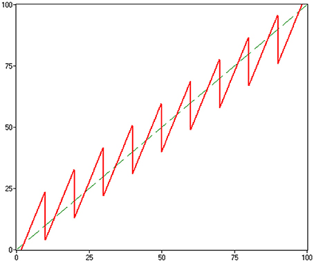
Figure 7. The shape of the map if the price domain is subdivided in interval of length equal to 10. The values of the parameters are: a = 1, f = 0.1, c = 2, and F = 50.

Obviously, the number of regimes is arbitrary. They obtain timeplots similar to the one represented in Figure 8 and they show how all kinds of crisis can be replicated by such a model.

FIGURE 8

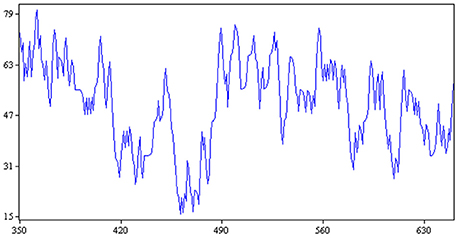
Figure 8. Timeplot obtained with the same values of the parameters of Figure 6 and initial condition P₀ = 54.

5. Conclusions

Agent-based financial market models are quite powerful in explaining the dynamics of financial markets. Since the main building blocks of these models are also based on empirical observations, they may be regarded as quite realistic descriptions of the actual price formation process of financial markets. The goal of our paper is to review some recent work on agent-based models in which the dynamics is driven by piecewise-linear maps. Besides presenting the seminal contribution of Huang and Day [21], we illustrate model extensions in which the trading behavior of the agents is more general and in which the agents' perception of the fundamental value evolves over time. As we have seen, these models are able to produce bubbles and crashes and excess volatility. Buffeted with dynamics noise, these models are even capable of replicating the finer details of the dynamics of financial markets.

Let us finally point out some avenues for future research.

• In our review, we have presented a few mechanisms that can lead to a piecewise-linear map. However, there may be more mechanism around. For instance, the behavior of the market maker hasn't received much attention so far. One may consider, for instance, that the market maker's price adjustment behavior depends on the market's distortion.

• Since piecewise-linear agent-based financial market models offer novel explanations for the emergence of bubbles and crashes and excess volatility, it is very natural to ask whether there are regulatory policies which may tame such kind of dynamics. For instance, one could imagine that there is a central authority who acts as a further player in the models we have presented in our paper, using a linear intervention (demand) function such as $D_t^A=r(F-P_t)$ with r > 0⁶. Unfortunately, not much work exists in this direction.

• Moreover, there are a number of regulatory policies which may itself create piecewise maps, either linear or not. Examples in this direction include, among others, the work on price limiters by He and Westerhoff [55], on short-selling constraints by Anufriev and Tuinstra [56] and on profit taxes by Schmitt and Westerhoff [57]. It seems that the mathematical progress which has been made in the analysis of piecewise-linear models may be used to revisit these models.

• Of course, even the existing models are still not completely understood. Without question, more work is needed to develop a better mathematical handling of them. In this sense we also mention that future work may attack in more detail models with more than two or three branches.

• The models we have presented in our review have in common that the trading rules of the traders formalize their orders and that a market maker adjusts the price of the asset with respect to the sum of these orders. One drawback of such a setup is that the positions of the traders and the market maker may become unreasonable high. In contrast, Brock and Hommes [17] develop a framework in which similar trading rules, derived from mean variance preferences, indicate the positions of traders. Moreover, Brock and Hommes [17] assume market clearing, i.e., the price of the risky asset adjusts such that demand is equal to supply, keeping the positions of the traders bounded. It might be worthwhile to develop the models we have presented here also in that direction.

• Moreover, Brock and Hommes [17] assume that traders switch between different trading rules (or different expectation schemes) according to an evolutionary fitness measure such as past realized profits. The switching rate of the traders depends on their intensity of choice. The higher the intensity of choice, the more sensitive the traders are in selecting the more attractive trading rule. However, if the intensity of choice approaches infinity, all traders simultaneously switch trading rules and the underlying map becomes piecewise defined. It seems to be worthwhile to explore also this aspect in more detail. Although it is an extreme assumption that the intensity of choice goes to infinity (sometimes referred to as the neoclassical limit), piecewise linear maps may allow clear-cut analytical insights in these situations which are otherwise precluded (see [52] for some ideas).

• The models we have presented in this paper are only concerned with the dynamics of a single risky asset. For simple multi-asset market models see e.g., Tramontana et al. [58] and Schmitt and Westerhoff [59]. Moreover, future work should try to extend these models such that they also interact with the real side of the economy. We venture that sharp transitions in the dynamics of financial markets will spill-over to the dynamics of the real economy.

• Recently, Schmitt and Westerhoff [60] derive a rather simple small-scale agent-based model out of a more complex large-scale agent-based model. It would be interesting to do the same for a piecewise-linear agent-based model. As we have seen in this paper, the dynamics of piecewise-linear models lives from the fact that the whole group of a trader type collectively changes its behavior. Having a microfounded model would allow to relax this assumption and to explore how some additional in-group-heterogeneity affects the dynamics. Analytical insights derived from simple piecewise-linear agent-based models maybe helpful to understand the functioning of more complex companion models.

• A few piecewise-linear agent-based financial market models have already been calibrated and demonstrate that they can mimic the dynamics of actual financial markets quite well. However, it is an important task to bring this line of work closer to the data. Since the building blocks of these models consist of linear equations, they may have a straightforward economic interpretation. Some inspiring work in this direction was already done by Day [61], albeit in a macroeconomic context.

To conclude, we hope that our paper stimulates more work in this exciting research direction.

Author Contributions

All authors listed, have made substantial, direct and intellectual contribution to the work, and approved it for publication.

Conflict of Interest Statement

The authors declare that the research was conducted in the absence of any commercial or financial relationships that could be construed as a potential conflict of interest.

The handling Editor declared a past co-authorship with one of the authors, FT, and states that the process nevertheless met the standards of a fair and objective review.

Footnotes

1. ^Obviously it makes sense when D_i and D_i+1 are contiguous.

2. ^Early studies on this topic can be found in Leonov [31, 32] and Mira [33, 34].

3. ^Actually they label them as α-investors and β-investors, but lately they have been more commonly called fundamentalists and chartists, respectively.

4. ^A sudden crisis is a crisis characterized by a sequence of important price drops, from a peak to the bottom. The price drop requires a very short time and the recovery is usually long. An example is the tulip crisis in 1637. A smooth crisis is characterized by a moderate but continuous and persistent price decrease, such as the Japanese crisis of 1990–2007. Finally, the disturning crisis is a sudden crash which follows a period of fluctuations with a negative trend. This kind of crisis is considered the most common and the most dangerous. The 2007–2009 global credit cruch is one of them.

5. ^Actually Huang and Zheng [23] endogenize the speed of adjustment of fundamentalists, but this is behind our purposes.

6. ^For instance, the average relative mispricing visible in the top panel of Figure 6 reduces from 10.80 percent for r = 0 to 3.51 percent for r = 0.01. This example illustrates the potential of such an intervention function. However, the impact of such an intervention function on the model dynamics may, in general, be much more intricate since it affects the slopes of all branches of the underlying map. While some branches of the map may give rise to more stable dynamics, others may not. It is also clear that small changes in the intervention parameter r may have significant effects on the dynamics (they may just turn a steady state stable or unstable). Clearly, this important aspect deserves more attention in future research. For some guidance in this direction see Westerhoff and Franke [54].

References

1. Kindleberger C. Manias, Panics and Crashes: A History of Financial Crises. New York, NY: Wiley (2000).

Google Scholar

2. Reinhart C, Rogoff K. This Time is Different. Princeton, NJ: Princeton University Press (2009).

Google Scholar

3. Shiller R. Irrational Exuberance. Princeton, NJ: Princeton University Press (2015).

Google Scholar

4. Mantegna R, Stanley E. An Introduction to Econophysics. Cambridge: Cambridge University Press (2000).

Google Scholar

5. Cont R. Empirical properties of asset returns: stylized facts and statistical issues. Quant Finan. (2001) 1:223–36. doi: 10.1080/713665670

CrossRef Full Text | Google Scholar

6. Lux T, Ausloos M. Market fluctuations i: scaling, multiscaling, and their possible origins. In: Bunde AKJ, Schellnhuber H, editors. Science of Disaster: Climate Disruptions, Heart Attacks, and Market Crashes. Berlin: Springer-Verlag (2002). p. 373–410.

7. Chiarella C, Dieci R, He XZ. Heterogeneity, market mechanisms, and asset price dynamics. In: Hens T, Schenk-Hoppé K, editors. Handbook of Financial Markets: Dynamics and Evolution. North-Holland: Amsterdam (2009). p. 277–344.

8. Hommes C, Wagener F. Complex evolutionary systems in behavioral finance. In: Hens T, Schenk-Hoppé K, editors. Handbook of Financial Markets: Dynamics and Evolution. North-Holland: Amsterdam (2009). p. 217–276.

9. Lux T. Stochastic behavioural asset-pricing models and the stylized facts. In: Hens T, Schenk-Hoppé K, editors. Handbook of Financial Markets: Dynamics and Evolution. North-Holland: Amsterdam (2009). p. 161–216.

10. Hommes C. The heterogeneous expectations hypothesis: some evidence from the lab. J Econ Dyn Control (2011) 35:1–24. doi: 10.1016/j.jedc.2010.10.003

CrossRef Full Text | Google Scholar

11. Menkhoff L, Taylor M. The obstinate passion of foreign exchange professionals: technical analysis. J Econ Literat. (2007) 45:936–72. doi: 10.1257/jel.45.4.936

CrossRef Full Text | Google Scholar

12. Murphy J. Technical Analysis of Financial Markets. New York, NY: New York Institute of Finance (1999).

13. Graham B, Dodd D. Security Analysis. New York, NY: McGraw-Hill (1951).

Google Scholar

14. Day R, Huang W. Bulls, bears and market sheep. J Econ Behav Organ. (1990) 14:299–329. doi: 10.1016/0167-2681(90)90061-H

CrossRef Full Text | Google Scholar

15. De Grauwe P, Dewachter H, Embrechts M. Exchange Rate Theory – Chaotic Models of Foreign Exchange Markets. Oxford: Blackwell (1993).

Google Scholar

16. Lux T. Herd behaviour, bubbles and crashes. Econ J. (1995) 105:881–96. doi: 10.2307/2235156

CrossRef Full Text | Google Scholar

17. Brock W, Hommes C. Heterogeneous beliefs and routes to chaos in a simple asset pricing model. J Econ Dyn Control (1998) 22:1235–74. doi: 10.1016/S0165-1889(98)00011-6

CrossRef Full Text | Google Scholar

18. Farmer D, Joshi S. The price dynamics of common trading strategies. J Econ Behav Organ. (2002) 49:149–71. doi: 10.1016/S0167-2681(02)00065-3

CrossRef Full Text | Google Scholar

19. Chiarella C, Dieci R, Gardini L. The dynamic interaction of speculation and diversification. Appl Math Finan. (2005) 12:17–52. doi: 10.1080/1350486042000260072

CrossRef Full Text | Google Scholar

20. Franke R, Westerhoff F. Structural stochastic volatility in asset pricing dynamics: estimation and model contest. J Econ Dyn Control (2012) 36:1193–211. doi: 10.1016/j.jedc.2011.10.004

CrossRef Full Text | Google Scholar

21. Huang W, Day, R. Chaotically switching bear and bull markets: the derivation of stock price distributions from behavioral rules. In: Day R, Chen P, editors. Nonlinear Dynamics and Evolutionary Economics. Oxford: Oxford University Press (1993). p. 169–182.

22. Huang W, Zheng H, Chia W. Financial crisis and interacting heterogeneous agents. J Econ Dyn Control (2010) 34:1105–122. doi: 10.1016/j.jedc.2010.01.013

CrossRef Full Text | Google Scholar

23. Huang W, Zheng H. Financial crisis and regime-dependent dynamics. J Econ Behav Organ. (2012) 82:445–61. doi: 10.1016/j.jebo.2012.02.008

CrossRef Full Text | Google Scholar

24. Tramontana F, Westerhoff F, Gardini L. On the complicated price dynamics of a simple one-dimensional discontinuous financial market model with heterogeneous interacting traders. J Econ Behav Organ. (2010a) 74:187–205. doi: 10.1016/j.jebo.2010.02.008

CrossRef Full Text | Google Scholar

25. Tramontana F, Westerhoff F, Gardini L. The bull and bear market model of huang and day: some extensions and new results. J Econ Dyn Control (2013) 37:2351–70. doi: 10.1016/j.jedc.2013.06.005

CrossRef Full Text | Google Scholar

26. Nusse H, Yorke J. Border-collision bifurcations including period two to period three for piecewise smooth systems. Physica D (1992) 57:39–57. doi: 10.1016/0167-2789(92)90087-4

CrossRef Full Text | Google Scholar

27. Nusse H, Yorke J. Border-collision bifurcation for piecewise smooth one-dimensional maps. Int J Bifurcat Chaos (1995) 5:189–207. doi: 10.1142/S0218127495000156

PubMed Abstract | CrossRef Full Text | Google Scholar

28. Maistrenko Y, Maistrenko V, Chua L. Cycles of chaotic intervals in a timedelayed chua's circuit. Int J Bifurcat Chaos (1993) 3:1557–72.

Google Scholar

29. Maistrenko Y, Maistrenko V, Vikul S, Chua L. Bifurcations of attracting cycles from time-delayed chua's circuit. Int J Bifurcat Chaos (1995) 5:653–71.

Google Scholar

30. Maistrenko Y, Maistrenko V, Vikul S. On period-adding sequences of attracting cycles in piecewise linear maps. Chaos Solit Fract. (1998) 9:67–75. doi: 10.1016/S0960-0779(97)00049-0

CrossRef Full Text | Google Scholar

31. Leonov N. Map of the line onto itself. Radiofisica (1959) 2:942–56.

PubMed Abstract

32. Leonov N. Discontinuous map of the straight line. Dokl Acad Nauk SSSR (1962) 143:1038–41.

33. Mira C. Sur les structure des bifurcations des diffeomorphisme du cercle. C R Acad Sci Paris Ser A (1978) 287:883–6.

34. Mira C. Chaotic Dynamics. Singapore: World Scientific (1987). doi: 10.1142/0413

CrossRef Full Text | Google Scholar

35. Avrutin V, Gardini L, Schanz M, Sushko I, Tramontana F. Continuous and Discontinuous Piecewise-Smooth One-Dimensional Maps: Invariant Sets and Bifurcation Structures. Singapore: World Scientific (2016).

36. Banerjee S, Karthik M, Yuan G, Yorke J. Bifurcations in one-dimensional piecewise smooth maps - theory and applications in switching circuits. IEEE Trans Circuits Syst I Fund Theory Appl. (2000a) 47:389–94. doi: 10.1109/81.841921

CrossRef Full Text

37. Banerjee S, Ranjan P, Grebogi C. Bifurcations in 2d piecewise smooth maps - theory and applications in switching circuits. IEEE Trans Circuits Syst I Fund Theory Appl. (2000b) 47:633–64. doi: 10.1109/81.847870

CrossRef Full Text | Google Scholar

38. Feely O, Fournier-Prunaret D, Taralova-Roux I, Fitzgerald D. Nonlinear dynamics of bandpass sigma-delta modulation. An investigation by means of the critical lines tool. Int J Bifurcat Chaos (2000) 10:303–27. doi: 10.1142/S0218127400000207

CrossRef Full Text | Google Scholar

39. Fournier-Prunaret D, Feely O, Taralova-Roux I. Lowpass sigma-delta modulation: an analysis by means of the critical lines tool. Nonlin Anal. (2001) 47:5343–55. doi: 10.1016/S0362-546X(01)00639-3

CrossRef Full Text | Google Scholar

40. Zhusubaliyev Z, Soukhoterin E, Mosekilde E. Quasiperiodicity and torus breakdown in a power electronic dc/dc converter. Math Comput Simul. (2007) 73:364–77. doi: 10.1016/j.matcom.2006.06.021

CrossRef Full Text | Google Scholar

41. Bischi G, Merlone U. Global dynamics in binary choice models with social influence. J Math Soc. (2009) 33:277–302. doi: 10.1080/00222500902979963

CrossRef Full Text | Google Scholar

42. Dal Forno A, Gardini L, Merlone U. Ternary choices in repeated games and border collision bifurcations. Chaos Solit Fract. (2012) 45:294–305. doi: 10.1016/j.chaos.2011.12.003

CrossRef Full Text | Google Scholar

43. Puu T, Sushko I. Business Cycle Dynamics, Models and Tools. New York, NY: Springer-Verlag (2006). doi: 10.1007/3-540-32168-3

CrossRef Full Text | Google Scholar

44. Sushko I, Puu T, Gardini L. The hicksian floor-roof model for two regions linked by interregional trade. Chaos Solit Fract. (2003) 18:593–612. doi: 10.1016/S0960-0779(02)00679-3

CrossRef Full Text | Google Scholar

45. Gardini L, Sushko I, Naimzada A. Growing through chaotic intervals. J Econ Theory (2008) 143:541–57. doi: 10.1016/j.jet.2008.03.005

CrossRef Full Text | Google Scholar

46. Puu T, Sushko I. Oligopoly Dynamics, Models and Tools. New York, NY: Springer-Verlag (2002). doi: 10.1007/978-3-540-24792-0

CrossRef Full Text

47. Tramontana F, Gardini L, Puu T. Duopoly games with alternative technologies. J Econ Dyn Control (2009a) 33:250–65. doi: 10.1016/j.jedc.2008.06.001

CrossRef Full Text

48. Day R. Complex dynamics, market mediation and stock price behavior. North Amer Actuar J. (1997) 1:6–21. doi: 10.1080/10920277.1997.10595622

CrossRef Full Text | Google Scholar

49. Tramontana F, Gardini L, Westerhoff F. Intricate asset price dynamics and one-dimensional discontinuous maps. In: Puu T, Panchuk A, editors. Nonlinear Economic Dynamics. New York, NY: Nova Science Publishers (2010b). p. 43–57.

50. Tramontana F, Gardini L, Westerhoff F. Heterogeneous speculators and asset price dynamics: further results from a one-dimensional discontinuous piecewise-linear map. Comput Econ. (2011) 38:329–47. doi: 10.1007/s10614-011-9284-9

CrossRef Full Text | Google Scholar

51. Tramontana F, Westerhoff F, Gardini L. One-dimensional maps with two discontinuity points and three linear branches: mathematical lessons for understanding the dynamics of financial markets. Decis Econ Finan. (2014) 37:27–51. doi: 10.1007/s10203-013-0145-y

CrossRef Full Text | Google Scholar

52. Tramontana F, Westerhoff F, Gardini L. A simple financial market model with chartists and fundamentalists: market entry levels and discontinuities. Math Comput Simul. (2015) 108:16–40. doi: 10.1016/j.matcom.2013.06.002

CrossRef Full Text | Google Scholar

53. Tramontana F, Westerhoff F. One-dimensional discontinuous piecewise-linear maps and the dynamics of financial markets. In: Bischi GI, Chiarella C, Sushko I, editors. Global Dynamics in Economics and Finance. Essays in Honour of Laura Gardini. Berlin: Springer-Verlag (2013). p. 205–222. doi: 10.1007/978-3-642-29503-4_9

CrossRef Full Text

54. Westerhoff F, Franke R. Agent-based models for economic policy design: two illustrative examples. In: Chen SH, Kaboudan M, Du YR, editors. OUP Handbook on Computational Economics and Finance. Oxford: Oxford University Press (2016).

55. He XZ, Westerhoff F. Commodity markets, price limiters and speculative price dynamics. J Econ Dyn Control (2005) 29:1577–96. doi: 10.1016/j.jedc.2004.09.003

CrossRef Full Text | Google Scholar

56. Anufriev M, Tuinstra J. The impact of short-selling constraints on financial market stability in heterogeneous agents model. J Econ Dyn Control (2013) 37:1523–43. doi: 10.1016/j.jedc.2013.04.015

CrossRef Full Text | Google Scholar

57. Schmitt N, Westerhoff F. Managing rational routes to randomness. J Econ Behav Organ. (2015) 116:157–73. doi: 10.1016/j.jebo.2015.04.018

CrossRef Full Text | Google Scholar

58. Tramontana F, Gardini L, Dieci R, Westerhoff F. The “bull and bear” dynamics in a nonlinear model of interacting markets. Discrete Dyn Nat Soc. (2009b) 2009:310471. doi: 10.1155/2009/310471

CrossRef Full Text | Google Scholar

59. Schmitt N, Westerhoff F. Speculative behavior and the dynamics of interacting stock markets. J Econ Dyn Control (2014) 45:262–88. doi: 10.1016/j.jedc.2014.05.009

CrossRef Full Text | Google Scholar

60. Schmitt N, Westerhoff F. Heterogeneity, spontaneous coordination and extreme events within large-scale and small-scale agent-based financial market models. BERG Working Paper No. 111, University of Bamberg (2016).

Google Scholar

61. Day R. Complex Economic Dynamics. Volume II: An Introduction to Macroeconomic Dynamics. Boston, MA: MIT Press (1999).