Maps with Vanishing Denominator and Their Applications

1. Introduction

In this paper we consider a particular class of maps that are not defined in the whole space. In particular, we summarize the results concerning two-dimensional maps not defined in the whole plane because of the presence of a denominator that can vanish. These maps are called maps with vanishing denominator and the consequences of their features for the global properties of such maps have already been surveyed (see for instance 1 and more recently 2). What differentiates this survey from the others is the focus on the different fields of application of such maps. We will survey applications in Biology and Ecology, besides the well-known application to Economics (already surveyed in 2) and we also show how maps with vanishing denominator may appear in a class of fractional rational maps that may have multiple practical applications. The aim is to stimulate researchers in various fields to check if some particular global feature of their maps can be the consequence of a map with vanishing denominator and to provide some tools to explain them. In fact, as a consequence of the presence of a vanishing denominator, the attractors and/or the basins of attraction of the coexisting locally stable invariant sets may assume quite complicated shapes, making extremely difficult to predict what may occur at the trajectory after a slight change of the initial value or after a variation of a prameter's value. The paper proceeds as follows: in Section 2 we introduce the most important definitions and the main results; Section 3 is devoted to the applications while in Section 4 we make some conclusions.

2. General Definitions and Properties

In the section we recall some preliminary definitions related to maps with vanishing denominator. Definitions and results of this section come from Bischi et al. [3, 4] even if some earlier results can also be found in Mira [5, 6].

Definition 1. A map with vanishing denominator is a map of ℝⁿ with n ≥ 2, that is not defined in the whole space ℝⁿ because at least one of its components contains a denominator which can vanish.

To make simpler the notation we only refer to the case where only one component of the map is characterized by a vanishing denominator. Nevertheless, the results still hold when both the components take the form 0/0. In such a case a map T with vanishing denominator takes the following form

$\begin{array}{ll}T:\{\begin{array}{l}{x}^{\prime }=F(x,y)\hfill \\ y^{\prime }=G(x,y)=\frac{N(x,y)}{D(x,y)}\hfill \end{array}\hfill & (1)\hfill \end{array}$

where the continuously differentiable functions F(x, y), N(x, y) and D(x, y) have not common factors and are defined in the whole plane ℝ². To make the notation simpler we only refer to the case where only one component of the map is characterized by a vanishing denominator. Nevertheless, the results still hold when both the components may take the form 0/0.

Since the G component of the map features a denominator, the following general definition is introduced:

Definition 2. The set of points (δ_s) where the denominator vanishes, that is:

${\delta }_s=\{(x, y)\in {ℝ}^2|D(x, y)=0\}$

is called set of nondefinition of the map T.

The set of nondefinition is usually made up by the union of smooth curves of the plane.

We are interested in studying what occurs with the application of the map T to bounded and smooth arcs γ that are transverse to the set of nondefinition.

First of all we can parametrize the arc as γ(τ), such that γ(0) = (x₀, y₀) denotes the intersection between γ(τ) and δ_s. So we have that D(x₀, y₀) = 0.

Two cases must be considered separately:

– if N(x₀, y₀) ≠ 0 then we have that the image of the arc γ will be characterized by a vertical asymptote in x = F(x₀, y₀), that is:

$\underset{\tau \to 0\pm }{\lim }T(\gamma (\tau ))=(F(x_0,y_0),\infty )$

with ∞ denoting either +∞ or −∞.

– if N(x₀, y₀) = 0 then it is no longer certain that the image of γ will have a vertical asymptote, because in such a case the component G(x, y) of the map takes the form 0/0 and its limit may be finite.

In this last case the point (x₀, y₀) is called “focal point”:

Definition 3. A two-dimensional map T owns a focal point Q = (x₀, y₀) if at least one component of the map takes the form 0/0 in Q, and considering simple smooth arcs γ(τ) with γ(0) = 0, we have that $\underset{\tau \to 0}{\lim }T\left(\gamma \left(\tau \right)\right)$ is finite.

In correspondence with a focal point Q, the image T(γ) is a bounded arc passing through the point:

$\left(F(x_0,y_0),\underset{\tau \to 0}{\lim }G\left(x(\tau ),y(\tau )\right)\right)$

Figure 1 qualitatively represents both cases.

FIGURE 1

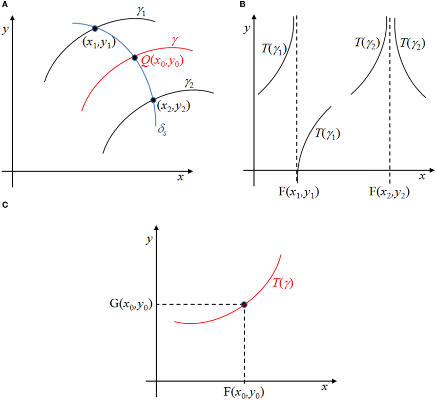
Figure 1. The action of the map T on arcs transverse to the set of nondefinition (A) is different. If N(x, y) does not vanish when the denominator D(x, y) vanishes (or it does but the limit of the ratio is infinite) then the image of the arc is the union of two arcs separated by a vertical asymptote (B). If both N(x, y) and D(x, y) vanish at the intersection and the limit of the ratio is finite, then the image is a continuous arc (C).

Definition 4. The prefocal set δ_Q is the set of all finite values assumed by $\underset{\tau \to 0}{\lim }T\left(\gamma \left(\tau \right)\right)$ taking different arcs γ(τ) through Q.

In the case of the two-dimensional map (1), the equation of the prefocal set is given by x = F(Q).

Focal points are further distinguished into two classes: simple and not simple. In order to understand the difference between them we must introduce the four partial derivatives of N(x, y) and D(x, y):

$\begin{array}{cc}{\overline{N}}_x=\frac{\partial N}{\partial x}(x_0,y_0)& {\overline{N}}_y=\frac{\partial N}{\partial y}(x_0,y_0)\\ {\overline{D}}_x=\frac{\partial D}{\partial x}(x_0,y_0)& {\overline{D}}_y=\frac{\partial D}{\partial y}(x_0,y_0)\end{array}$

Definition 5. A focal point Q = (x₀, y₀) is called simple iff:

${\overline{N}}_x{\overline{D}}_y-{\overline{N}}_y{\overline{D}}_x\ne 0,$

otherwise it is called not simple.

2.1. The Role of the Map

When the focal point is simple there exists a one-to-one correspondence between the slope m of the arc γ in Q and the point (F(Q), y) in which its image T(γ) crosses the prefocal set δ_Q. As a consequence, different arcs γ_j crossing the set of nondefinition in Q with different slopes m_j are mapped by T into bounded arcs T(γ_j) crossing the prefocal set δ_Q in different points (see Figure 2).

FIGURE 2

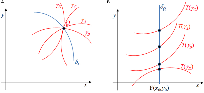
Figure 2. Arcs crossing the focal point with different slopes (A) are mapped into arcs crossing the prefocal set in different points (B).

In particular, let us consider a smooth simple arc γ crossing the set of nondefinition δ_s in Q, represented as:

$\gamma (\tau ):\{\begin{array}{l}x(\tau )=x_0+{\xi }_1\tau +{\xi }_2{\tau }^2+...\hfill \\ y(\tau )=y_0+{\eta }_1\tau +{\eta }_2{\tau }^2+...\hfill \end{array}\tau \ne 0,$

and let us assume the following smooth functions:

$\begin{array}{l}N(x,y)={\overline{N}}_x(x-x_0)+{\overline{N}}_y(y-y_0)+O_2\hfill \\ D(x,y)={\overline{D}}_x(x-x_0)+{\overline{D}}_y(y-y_0)+O_2^{\prime }\hfill \end{array}$

with O₂ and $O_2^{\prime }$ as higher order terms.

Provided that Q is a simple focal point, we have that:

$\underset{\tau \to 0}{\lim }\frac{N(\gamma (\tau ))}{D(\gamma (\tau ))}=\frac{{\overline{N}}_x{\xi }_1+{\overline{N}}_y{\eta }_1}{{\overline{D}}_x{\xi }_1+{\overline{D}}_y{\eta }_1}$

which permits to obtain explicitly the one-to-one correspondence between the slope m of the arc γ through Q and the second coordinate of the point where its image crosses δ_Q:

$m\to \left(F(Q),y(m)\right),\text{ with }y(m)=\frac{{\overline{N}}_x+m{\overline{N}}_y}{{\overline{D}}_x+m{\overline{D}}_y}$

with m = η₁/ξ₁.

2.2. Noninvertible Maps and the Role of the Inverses

Before deepening the role of the inverse (or the inverses) of the map T, we must introduce noninvertible maps. When a map T is noninvertible, then the phase space can be subdivided into open zones Z_k made up by points having k distinct rank-1 preimages. These preimages can be obtained through the application of k inverse maps. So, for any (x, y) belonging to Z_k, there exist k inverses $T_j^{-1}$, j = 1, …, k, such that we can find k distinct points (x_j, y_j), j = 1…, k mapped into (x, y) by the map T [i.e., T(x_j, y_j) = (x, y) and $T_j^{-1}(x,y)=(x_j,y_j)$)]. Following the notation introduced by Gumowski and Mira [7], we call critical set LC (from the French “Ligne Critique”), the locus of points having at least two coincident rank-1 preimages. Merging preimages are located in another set of points called LC₋₁ that is included in the set of points J₀ in which the determinant of the Jacobian matrix of T vanishes:

$L{C}_{-1}\subseteq J_0=\left\{\left(x,y\right)\in {ℝ}^2|\det J(T)=0\right\}$

In fact, in any neighborhood of LC₋₁ we can find at least two distinct points mapped by T into the same point. As a consequence, the map T is not locally invertible in LC₋₁.

The zones Z_k are separated by segments of the critical curve LC = T(LC₋₁).

Dealing with a map with vanishing denominator the role of the inverse or inverses (if the map is invertible or noninvertible, resp.) is particularly important.

If our map T is an invertible map, then a unique focal point Q can be associated to the prefocal curve δ_Q. Whenever a smooth segment of a curve ω moves toward δ_Q, its preimage ${\omega }_{-1}=T^{-1}(\omega )$ approaches the focal point Q. When ω becomes tangent to the prefocal curve, ω₋₁ has a cusp in Q, where two arcs of common slope given by m(y_c) join each other. If the segment ω crosses δ_Q the consequence is that the two portions of the arc intersecting the prefocal curve are both mapped into arcs through the focal point (with different slopes) by the inverse map T⁻¹, forming a loop.

It is also worth to introduce a further definition that we will employ along the rest of the paper.

Definition 6. A basin of attraction ${B}$(A) of an attracting set A is defined as the set of points p whose forward trajectories converge to A, i.e.,

${B}(A)=\{p:M^t(p)\to A,ast\to \infty \}$

where M : ℝⁿ → ℝⁿ.

Let us consider the boundary of a basin of attraction and let us assume that, by varying the value of some parameters, this boundary approaches, has a contact, and then crosses a prefocal curve. As a consequence, the preimage of such a basin boundary, through the action of the inverse T⁻¹, gives rise to the creation of a cusp point in correspondence of the focal point Q (at the contact) and then creates a loop (after the contact, see Figure 3).

FIGURE 3

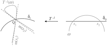
Figure 3. Creation of a lobe.

These loops are called lobes:

Definition 7. A lobe is the particular shape taken by a basin boundary after the bifurcation occurring when the boundary crosses a prefocal curve.

If a noninvertible map is characterized by focal points not located on LC₋₁, then a contact of LC with the border of the basin is related with the contact of two lobes on LC₋₁. The particular structure of the basin originated by such a contact is called crescent (see Figure 4). Crescents may arise also as a consequence of a contact between a lobe and a focal point different from the one from which the lobe has been created. This scenario may occur whenever the focal points of a noninvertible map are located on LC₋₁.

FIGURE 4

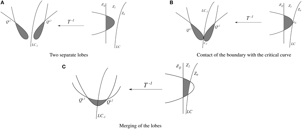
Figure 4. The creation of crescents as the result of merging of lobes. (A) Two separate lobes. (B) Contact of the boundary with the critical curve. (C) Merging of the lobes.

Definition 8. A crescent is a particular shape taken by a basin boundary in noninvertible maps as a consequence of:

– The contact of two lobes on LC₋₁ and is bounded by the two focal points that originated the lobes (when focal points are not located on LC₋₁);

– The contact of a lobe with a focal point different from the one from which it is originated (when focal points are located on LC₋₁).

3. Applications of the Main Results to Different Fields

In this section we provide some examples of applications in several fields of the global results concerning maps with vanishing denominator. We start from a rational map coming from the Bairstow's method that potentially may have a lot of applications. Then we proceed with applications to Economics, Biology and Ecology. The results presented in this section make use of the theoretical results previously discussed and also obtained in the papers by Gardini et al. [8], Bischi and Naimzada [9], Gu and Hao [10], and Gu and Huang [11]. The aim is to stimulate researchers from various fields to study the global properties of their maps with vanishing denominator.

3.1. The Gardini, Bischi and Fournier-Prunaret Model

The work by Gardini et al. [8] considers a class of two-dimensional non-invertible maps, characterized by the existence of a vanishing denominator: therefore the iterative process is not defined in a zero-measure subset of the plane. In particular, the analyzed map is obtained by the application of the Bairstow's method (an iterative numerical algorithm to find roots of polynomials) to a cubic equation. The dynamic behavior and the geometric properties of a two-dimensional map coming from the Bairstow's method are strongly influenced by the fact that a noninvertible map is considered and a fractional rational map has a vanishing denominator. The existence of a vanishing denominator, as we have seen in the previous section, implies that there is a subset of the plane where the map is not defined (the so-called singular set), and such a subset may include points in which also a numerator vanishes, so that the map takes the form 0/0, which are candidate to be focal points.

The two-dimensional map considered by the authors is defined as

$\begin{array}{ll}T:\{\begin{array}{l}u\prime =\frac{u^3+u(v-a+1)+a}{2u^2+v}\hfill \\ v\prime =\frac{v(u^2+a-1)+2au}{2u^2+v}\hfill \end{array}\hfill & (2)\hfill \end{array}$

The function T is defined on the domain ${ℝ}^2\backslash {\delta }_s$, where δ_s is the singular set formed by the points of the parabola

$\begin{array}{ll}{\delta }_s=\{(u,v)\in {ℝ}^2:v=-2u^2\}\hfill & (3)\hfill \end{array}$

Blish and Curry [12] shown that for a < 1/4 the map T has three distinct fixed points given by $R_1=(u_1^{*},v_1^{*})=(1,a)$, $R_2=(u_2^{*},u_3^{*})$, $R_3=(u_3^{*},u_2^{*})$ where

$u_2^{\ast }=\frac{-1+\sqrt{1-4a}}{2},u_3^{\ast }=\frac{-1-\sqrt{1-4a}}{2}$

are the real roots of the quadratic equation u² + u + a = 0.

In order to analyze and explain the qualitative basins structure, we shall make use of the fact that the map T is non-invertible and that it has a vanishing denominator. We recall that a non-invertible map T:(x, y) → (x′, y′) is characterized by the fact that the rank-1 preimages T⁻¹(x′, y′) of a given point (x′, y′) may be more than one. This implies that the plane can be subdivided into regions Z_k, k > 0, whose points have k distinct rank-1 preimages.

As recalled in the Introduction, many global dynamical properties of two-dimensional maps can be explained by the analysis of new kinds of singularities, such as the sets where a denominator of the map (or some of its inverses) vanishes, the points where the map (or some of its inverses) takes the form 0/0 in at least one component, and the prefocal curves. For the map T a situation in which not only the denominator D but also the two numerators N₁ and N₂ of the map T vanish in the point (u₀, v₀) ∈ δ_s, i.e., D(u₀, v₀) = N₁(u₀, v₀) = N₂(u₀, v₀) = 0 always occurs in the point

$Q_1=(1,-2)$

and, for a < 1/4, also in the points

$Q_2=(u_2^{\ast },-2u_2^{\ast }{}^2)Q_3=(u_3^{\ast },-2u_3^{\ast }{}^2).$

The equation of the prefocal set δ_Q1 is given by

$\begin{array}{ll}{\delta }_{Q_1}:v=2u-2+a\hfill & (4)\hfill \end{array}$

Furthermore, for a < 1/4, the equations of the prefocal lines δ_Qi, i = 2, 3, associated with the two additional focal points $Q_i=(u_i^{*},{-2u_i^{*}}^2)$, i = 2, 3, are

$\begin{array}{ll}{\delta }_{Q_i}=v=2u_i^{\ast }u+(u_i^{\ast }+2a-1),i=2,3\hfill & (5)\hfill \end{array}$

As remarked above, in order to describe in detail the basins' boundaries of the map, we consider the set of nondefinition δ_s (and its preimages). In Figure 5A we display, with different colors, the basins of attraction of the three fixed points. Consider the arc $T^{-1}({\delta }_{s,l})$: it crosses the prefocal line δ_Q1 in two points (only the upper one is visible in the figure). Thus, its rank-1 preimage on the right must be a loop issuing from the focal point Q₁, as the authors qualitatively explain in their paper. The same happens for the infinite sequence of preimages having a “parabolic” shape that are located on the left (i.e., in the half-plane u < 0). This generates infinitely many lobes of different basins issuing from the focal point Q₁, as the enlargement of Figure 5B reports.

FIGURE 5

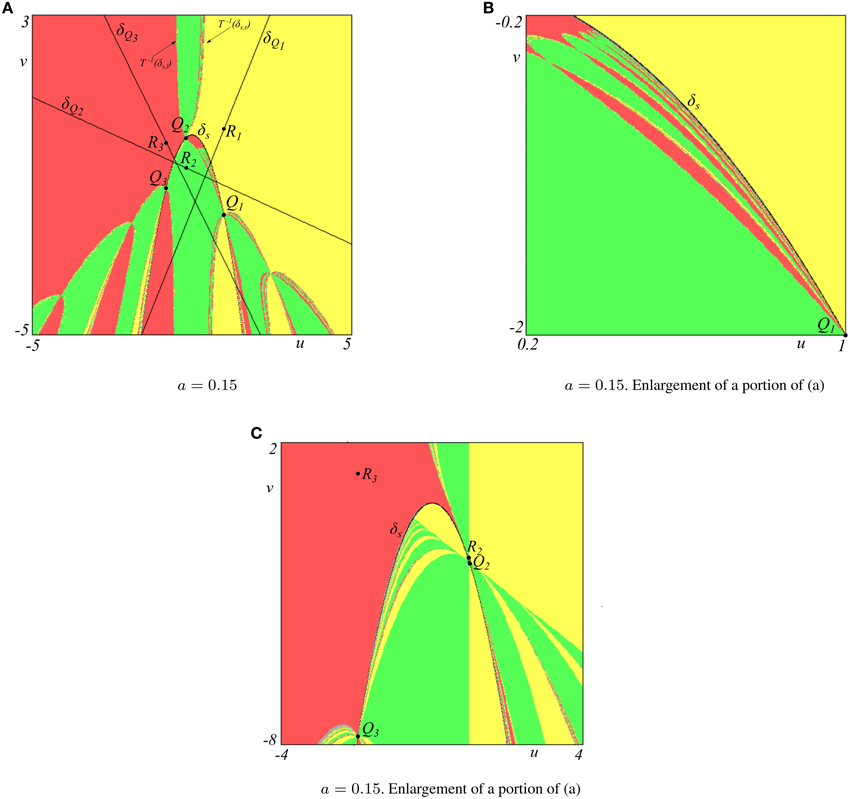
Figure 5. (A) The three basins of attraction of the fixed points are represented with different colors. The yellow region represents the points belonging to the basin of R₁, the green color represents the points belonging to the basin of R₂ while the red color represents the points belonging to the basin of R₃. The points Q₁, Q₂, and Q₃ are the focal points. (B,C) display two enlargements of (A) with infinitely many lobes issuing from the focal points.

Analogously, the preimage $T^{-1}({\delta }_{s,r})$ intersects the prefocal line δ_Q3 in two points, forming an arc, and its rank-1 preimage has a “loop” issuing from the focal point Q₃, and so on for the other curves, constituting a fan, intersecting the prefocal line δ_Q3 in arcs, giving rise to infinitely many lobes of the three basins issuing from the focal point Q₃, shown in Figure 5C.

From Figure 5A it can be seen the different role played by the focal point Q₂ with respect to the other two focal points. In fact Q₂ ∈ Z₀, that is it has no preimage: thus whenever some arc crosses through the prefocal line δ_Q2 its preimage gives rise to an arc through the focal point Q₂ and here the sequence of preimages stops. The property that Q₂ ∈ Z₀ holds for −2 < a < 1/4, while for a < −2 we have Q₂ ∈ Z₂ and Q₁ ∈ Z₀, i.e., the role of these two focal points is switched at a = −2. In fact, as the parameter a is decreased, at the value a = 0 we have Q₂ = (0, 0) ∈ Z₀, which is also a value with a particular symmetric structure in the basins, and then, for a < 0, the focal point Q₂ moves on the right side toward Q₁. At a = −2 we have R₁ = R₂ = Q₁ = Q₂. Then, for a = −2 a “change of role” between the couples R₁, Q₁ and R₂, Q₂ occurs, as now it is Q₁ the focal point in Z₀ (with no preimages) while Q₂ ∈ Z₂ has infinitely many preimages. Figure 6A displays the structure of the basins just before the bifurcation, while in Figure 6B, obtained just after the bifurcation, it is evident that a generic point (u₀, v₀) which belongs to the basin of R₁ for a > −2 belongs to the basin of R₂ for a < −2.

FIGURE 6

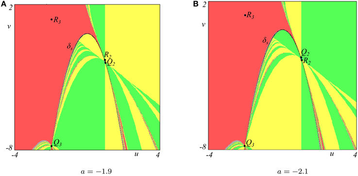
Figure 6. Basins of attraction of the fixed points. (A) a = −1.9, just before the bifurcation occurring at a = −2. (B) a = −2.1, just after the bifurcation occurring at a = −2.

3.2. The Bischi and Naimzada Model

Bischi and Naimzada [9] studied a nonlinear model with learning where agents are endowed with a fading memory (i.e., they take into consideration a weighted average of the past values with exponentially decreasing weights). In this model agents form expectations about a particular market price by using past prices information. The delimitation of the boundary that separates the set of initial conditions that generate trajectories converging to the equilibrium price (the Rational Expectations Equilibrium, REE) from the set of initial conditions that generate unbounded trajectories is the main goal of their work. The particular basin's structure they found is a direct consequence of the presence of a vanishing denominator in the two-dimensional dynamical system, whose dynamic properties were studied in Bischi and Gardini [13, 14]. The model with fading memory used to analyze the dynamics of the price (z_t) is described by the two-dimensional map

$\begin{array}{ll}T:\{\begin{array}{l}z\prime =\frac{\rho Wz+\beta z^2+\delta }{1+\rho W}\hfill \\ W\prime =1+\rho W\hfill \end{array}\hfill & (6)\hfill \end{array}$

where the variable W is used to model the dynamics of fading memory of economic agents. Notice that the model requires positive values of W for being economic meaningful, as it is related to the parameter ρ ∈ [0, 1] which, in turn, regulates the memory of the learning mechanism. The map (6) is a rational map which is not defined in the whole plane, because the denominator of the first component vanishes on the line of equation (set of nondefinition)

${\delta }_s:W=-\frac{1}{\rho }$

The presence of a vanishing denominator influences the basin structure of the underlying economic model, making more complicated to predict the effects of a change in the parameters' values or in the initial conditions.

The first component of Equation (6) assumes the form 0/0 in two points

$Q_1=\left(\frac{1-\sqrt{1-4\beta \delta }}{2\beta };-\frac{1}{\rho }\right)Q_2=\left(\frac{1+\sqrt{1-4\beta \delta }}{2\beta };-\frac{1}{\rho }\right)$

From such focal points, fans of basins boundaries arise giving peculiar finger-shaped structures, i.e., the lobes. Both focal points are characterized by the same prefocal line

${\delta }_Q:W=0$

Figure 7A, obtained with ρ = 0.6, δ = 3 and β = −1.8, clearly shows that when an invariant set, such as a basin boundary, crosses the prefocal line, two lobes emerge simultaneously from the focal points. In particular, the basin's boundary of the fixed point p* is formed by the vertical segment ω, given by the portion of the line of equation z = Q₁ and its preimages ω₋₁, ω₋₂ and ω₋₃. The yellow area represents the set of points that generates trajectories converging to the fixed point while the gray-shaded area represents the set of points that gives diverging trajectories. For this set of parameters there are two lobes, bounded by the curves ω₋₃, issuing from the focal points Q₁ and Q₂. By reducing the value of β (β ≈ −2.118) the dynamics converge to a cycle of period 2, whose basin is depicted in cyan, and the lobes are tangent to the prefocal line (see Figure 7B) and other secondary lobes emerge from the focal points (see the enlargement in Figure 7C). Hence the basin boundary also includes higher rank preimages ω_−k, k > 2, of the line ω, which have loops that bound lobes issuing from the focal points Q₁ and Q₂. As the parameter β is further decreased, the lobes cross the prefocal line and the structure of the basin may become more complicated, as Figure 8 displays, where two different attractors are shown, namely a 3-cycle (Figure 8A) and a 3-pieces chaotic attractor (Figure 8B). This complicated structure is due to bifurcations occurring when ω_−k−1, belonging to the set T^−k−1(ω), becomes tangent to the prefocal line.

FIGURE 7

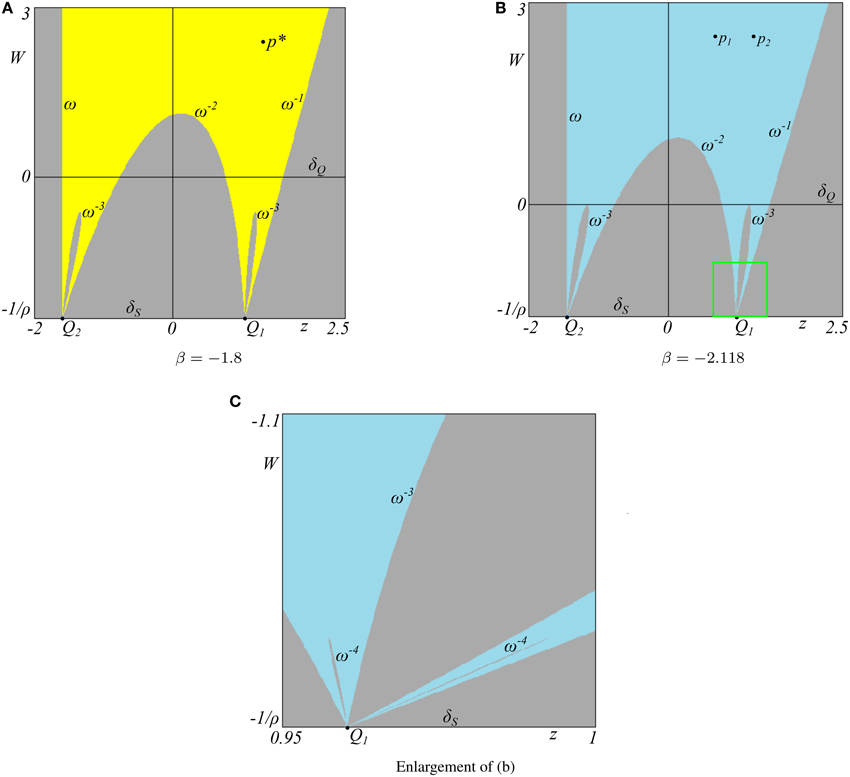
Figure 7. Phase space (z, W) of the map T and relative basins of attraction. The yellow basin denotes convergence to the fixed point (A) while the cyan basin denotes convergence to the 2-cycle (B). In (C) two further lobes issue from the focal point Q₁. Other parameter values are ρ = 0.6, δ = 3.

FIGURE 8

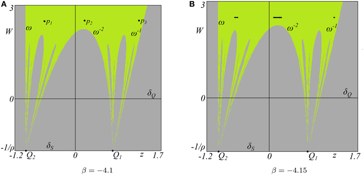
Figure 8. Phase space (z, W) of the map T and relative basins of attraction. In (A) the green basin denotes convergence to the 3-cycle while in (B) the green region refers to convergence to the chaotic attractor. Other parameter values are ρ = 0.6, δ = 3.

It is fundamental to underscore that without the global study of the map, involving the understanding of the origin of the complications derived from the presence of a vanishing denominator, it is almost impossible to completely foresee the effects of the parameters' variations.

3.3. The Gu and Hao Model

In 2007 Gu and Hao studied a simple two-dimensional map related to a discrete model of population generation [10]. A vanishing denominator is present in the inverse of the map, giving rise to the non-classical singularities surveyed in this paper: a set of nondefinition, a focal point and a prefocal line. The equation under study was the following dc-biased delayed regulation model

$\begin{array}{ll}v(t+1)=Av(t)(1-v(t-1))+E\hfill & (7)\hfill \end{array}$

where v(t) represents state of the nervous circuits, E indicates the dc-bias which is the effect of noise on the nervous circuits. Gu and Hao consider the model expressed by Equation (7) as a delayed regulation model with an external interference, v(t) is the k-th generation population density, A > 1 is the intrinsic or the maximum growth rate, and the parameter E can be associated to the external interference with an ecological population system. E can be considered as the immigrator part of populations from the outside or the one put in by human beings if E > 0, or as the part preyed by the external species if E < 0.

The model expressed by Equation (7) can be turned into a two-dimensional system by introducing the delayed variable u(t) = v(t−1) and, accordingly, the time evolution of the discrete dynamical system is obtained by the iteration of the two-dimensional map:

$\begin{array}{ll}M:\{\begin{array}{l}x\prime =y\hfill \\ y\prime =Ay(1-x)+E\hfill \end{array}\hfill & (8)\hfill \end{array}$

The map M has two real fixed points $P_{\pm }=(x_{\pm }^{*},x_{\pm }^{*})$ when $E>E_f=-{(A-1)}^2/4A$, where

$x_{\pm }^{\ast }=\frac{A-1\pm \sqrt{{(A-1)}^2+4AE}}{2A}$

P₋ is always an unstable saddle point while P₊ is stable for E > E_f Since M({y = 0}) = (0, E), the line y = 0 is focalized by the map M into a single point. Thus, it follows the map M has an inverse on the plane except on the line y = 0 (i.e., x′ = 0 according to the first Equation of 8) with the denominator, and such that Q = (0, E) is its focal point with the x-axis as a corresponding prefocal line δ_Q. In fact, the inverse of M is:

$\begin{array}{ll}{M}^{-1}:\{\begin{array}{l}x=1-\frac{y\prime -E}{Ax\prime }\hfill \\ y=x\prime \hfill \end{array}\hfill & (9)\hfill \end{array}$

For the map (9), the set of nondefinition δ_s coinciding with the locus of points in which the denominator of the first component of Equation (9) vanishes is given by:

${\delta }_s=\{(x\prime ,y\prime )\in {ℝ}^2:x\prime =0\}$

As we now, in the presence of a focal point the shape of the basins of attraction may be strongly influenced by it. For the parameter values A = 2.1 and E = −0.04, the fixed point $P_{+}=(x_{+}^{*},x_{+}^{*})$ is an unstable focus and an attractive closed invariant curve surrounds it. In Figure 9A the basin of attraction of the invariant curve is represented by the yellow region while the gray region represents the basin of infinity, i.e., the set of points that generate diverging trajectories. As A = 2.1 and E = 0.06995 the focal point Q becomes a saddle point of the map M. In fact, the invariant closed curve becomes the unstable manifold of Q due to the contact with Q, and the x-axis belongs to the stable manifold of Q (notice the equality M({y = 0}) = Q). When an invariant closed curve meets tangentially with the x-axis (i.e., with the prefocal line of the inverse M⁻¹ given by Equation 9), as shown in Figure 9B, it changes from a smooth curve to a non-smooth curve with a cusp at the focal point Q of the inverse (Equation 9). When the curve contacts transversely with the prefocal line of the inverse M⁻¹ (see Figure 9C obtained with A = 2.1 and E = 0.14), its rank-1 preimage under M⁻¹ forms a loop with a knot in Q by intersecting itself. It is noteworthy to mention that here the attractor is chaotic because the unstable manifold of a saddle point Q contacts transversely with its stable manifold (i.e., x-axis). This example reveals how the emergence of loops is not only related to the boundaries of some basin of attraction but it can also shape the whole aspect of an invariant set such as a chaotic attractor.

FIGURE 9

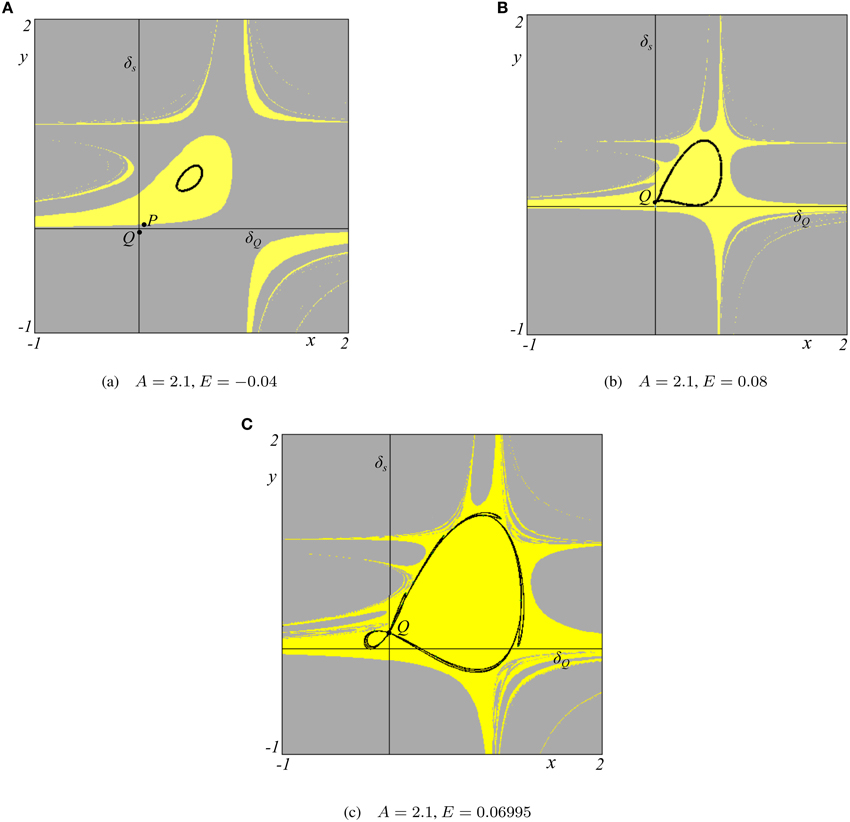
Figure 9. Basin of attraction (yellow color) and attractors for the model with external interference. The gray region represents the basin of unfeasible trajectories, namely all trajectories starting from the region converge to infinity. Point Q represents the focal point while P is the fixed point of the map. In (A) the basin of attraction of a closed invariant curve is represented. In (B) the invariant closed curve contacts tangentially with the prefocal line of the inverse M⁻¹ and in (C) the chaotic attractor is characterized by a knot of infinitely many curves that shrink into the focal point Q.

3.4. The Gu and Huang Model

Gu and Huang [11] considers a discrete predator-prey ecosystem and study the global properties of persistence in a biological model. The general aim of the authors is to show how the global dynamics can be analyzed by the study of some global bifurcations that change the structure of the domains of feasible trajectories as some parameters of the model are varied.

Let us briefly recall the main features of the model they consider. The discrete dynamical system under study is obtained by the iteration of the two-dimensional map

$\begin{array}{ll}T:\{\begin{array}{l}x\prime =Ax(1-x-y)\hfill \\ y\prime =Bxy\hfill \end{array}\hfill & (10)\hfill \end{array}$

where x represents the prey population and y the predator.

The map features three fixed points: Q = (0, 0) and P = ((A−1)/A, 0) located on the x-axis and the other E = (1/B, 1−1/B−1/A) is the only positive fixed point. One important feature of map (10) is that the y-axis is invariant, that is, T({x = 0}) = (0, 0) ∈ {x = 0}. It is immediate to see that the y-axis x = 0 is mapped into the point Q = (0, 0). This means that the predator species would be extinct because of the short food supply if the prey vanish. The coordinate axis x belongs to the invariant unstable manifold W^u of the saddle fixed point Q, since T(x, 0) = (x′, 0). Hence, the dynamics described by the map along the x-axis are governed by the one dimensional map x′ = f(x), where f is the restriction of T to the x-axis, and it is given by f(x) = Ax(1−x). From a biological point of view, this can be interpreted by the fact that the time evolution of prey, in the occurrence of the predator, the invader of prey, being extinct, is according to the logistic law.

Map T is a noninvertible map: in fact, a point (x′, y′) has two distinct preimages if Δ(x′, y′) = 1 − 4(x′/A+y′/B) > 0. Since T(x = 0) = (0, 0), we expect that the map T has at least one inverse with the denominator, and such that Q = (0, 0) is a focal point with the y-axis as a corresponding prefocal line δ_O. In fact, the inverses

$\begin{array}{ll}{T}_1^{-1}:\{\begin{array}{l}x=\frac{1}{2}(1+\sqrt{\Delta (x\prime ,y\prime )})\hfill \\ y=\frac{2y\prime }{B(1+\sqrt{\Delta (x\prime ,y\prime )})}\hfill \end{array}\hfill & (11)\hfill \end{array}$

and

$\begin{array}{ll}{T}_2^{-1}:\{\begin{array}{l}x=\frac{1}{2}(1-\sqrt{\Delta (x\prime ,y\prime )})\hfill \\ y=\frac{2y\prime }{B(1-\sqrt{\Delta (x\prime ,y\prime )})}\hfill \end{array}\hfill & (12)\hfill \end{array}$

are such that $T_2^{-1}$ has a focal point in Q = (0, 0) with the y-axis as a prefocal line. The set of nondefinition δ_s of the inverse $T_2^{-1}$ is given by

$\begin{array}{cc}{\delta }_s=\left\{(x\prime ,y\prime )\in {ℝ}^2: \frac{x\prime }{A}+\frac{y\prime }{B}=0\right\}& \left(13\right)\end{array}$

which coincides with the locus of points in which at least one (here the second component of $T_2^{-1}$) denominator vanishes. In general, the two-dimensional recurrence sequence obtained by the iteration of $T_2^{-1}$ is well defined provided that the initial condition belongs to the set

$E={ℝ}^2\backslash {\displaystyle \underset{k=0}{\overset{\infty }{\cup }}{T}^k}({\delta }_s)$

In fact, the points of the singular set must be excluded from the set of initial conditions that generate well defined sequences by the iteration of map $T_2^{-1}$, so that $T_2^{-1}:E\to E$.

In dynamical system theory, it is well known that if a singularity, as a cycle of any period, belongs to the boundary of some attracting set, then the whole stable set of the cycle also belongs to the boundary itself. Indeed, whenever this condition related to a cycle is not satisfied, it follows that some peculiarity exists, occurring at some bifurcation values. However, in the case of the singular sets described in the present model, such as straight lines mapped into one point, this property may be persistently not true.

For the map under scrutiny, it is easy to see that the y-axis x = 0 is mapped into the point Q = (0, 0). In this case, the knot Q is also the focal point of $T_2^{-1}$. In this example, we can find intervals of parameter values in which the focal point Q belongs to the boundary ∂B of a basin of attraction (of some attracting set in the positive quadrant of the phase plane). In Figure 10 we observe that the point Q belongs to the immediate basin of the attractor. The boundary ∂B exhibits a fractal structure, and infinitely many arcs of the boundary approach Q. Thus, Q is a limit point of arcs of the frontier, and it belongs to the frontier. However, it is not true that all the points which are mapped in Q by the map M, also belong to the frontier ∂B. In fact, it is immediate to see that there are several points of the line x = 0 which are not on the frontier of the basin. Thus:

$Q\in \partial B\nRightarrow T^{-1}(Q)\in B$

More precisely, we notice that Q is a singular fixed point of T because it is not a fixed point of the two inverses of T (for which it is a focal point). This may clarify the peculiar dynamic behavior at that point, shown in Figure 10.

FIGURE 10

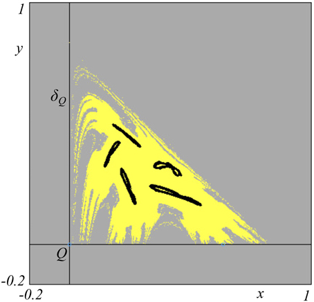
Figure 10. A cyclic chaotic attractor for the map T and its related basin of attraction (yellow color). The focal point Q is on the basin boundary, but the whole singular line δ_Q is not on the boundary. The gray region refers to unfeasible trajectories. Parameter values are: A = 4.22, B = 3.

4. Conclusions

Rational maps with vanishing denominator may appear in all applied fields. Usually these maps are characterized by global properties extremely complicated, especially if the map is noninvertible. In this paper we have not only surveyed the most important results concerning two-dimensional maps with vanishing denominator but we have also emphasized that they have been already applied in various contexts (from Economics to Biology and Ecology) to provide a deeper understanding on the formations of particular configurations of basins of attractions. We hope that researchers coming from all fields will include the global study of their maps with vanishing denominator by using the results and the procedures shown in this paper.

Author Contributions

All authors listed, have made substantial, direct and intellectual contribution to the work, and approved it for publication.

Conflict of Interest Statement

The authors declare that the research was conducted in the absence of any commercial or financial relationships that could be construed as a potential conflict of interest.

The handling Editor declared a past co-authorship with one of the authors, FT, and states that the process nevertheless met the standards of a fair and objective review.

References

1. Bischi GI, Gardini L, Mira C. Maps with a vanishing denominator. A survey of some results. Nonlin Anal Theory Methods Appl. (2001) 47:2171–85. doi: 10.1016/S0362-546X(01)00343-1

CrossRef Full Text | Google Scholar

2. Tramontana F. Maps with vanishing denominator explained through applications in Economics. J Phys Conf Ser. (2016) 692:012006. doi: 10.1088/1742-6596/692/1/012006

CrossRef Full Text | Google Scholar

3. Bischi GI, Gardini L, Mira C. Plane maps with denominator I: some generic properties. Int J Bifurcat Chaos (1999) 9:119–53. doi: 10.1142/S0218127499000079

CrossRef Full Text | Google Scholar

4. Bischi GI, Gardini L, Mira C. Plane maps with denominator. Part II: noninvertible maps with simple focal points. Int J Bifurcat Chaos (2003) 13:2253–77. doi: 10.1142/S021812740300793X

CrossRef Full Text | Google Scholar

5. Mira C. Singularités nonclassiques d'une récurrence et d'une équation différentielle d'ordre deux. Comptes Rendus Acad Sci Paris Ser I (1981) 292:146–51.

6. Mira C. Some properties of two-dimensional (Z₀ − Z₂) maps not defined in the whole plane. Grazer Math Berichte (1999) 339:261–78.

7. Gumowski I, Mira C. Recurrences and Discrete Dynamic Systems. Lecture Notes in Mathematics. Berlin: Springer Verlag (1980). doi: 10.1007/BFb0089135

CrossRef Full Text | Google Scholar

8. Gardini L, Bischi GI, Fournier-Prunaret D. Basin boundaries and focal points in a map coming from Bairstow's method. Chaos Interdiscip J Nonlin Sci. (1999) 9:367–80.

PubMed Abstract | Google Scholar

9. Bischi GI, Naimzada A. Global analysis of a nonlinear model with learning. Econ Notes Banca Monte Paschi Siena (1997) 26:445–76.

10. Gu EG, Hao YD. On the global analysis of dynamics in a delayed regulation model with an external interference. Chaos Solit Fract. (2007) 34:1272–84. doi: 10.1016/j.chaos.2006.05.079

CrossRef Full Text | Google Scholar

11. Gu EG, Huang Y. Global bifurcations of domains of feasible trajectories: an analysis of a discrete predator-prey model. Int J Bifurcat Chaos (2006) 16:2601–13. doi: 10.1142/S0218127406016288

CrossRef Full Text | Google Scholar

12. Blish SL, Curry JH. On the geometry of factorization algorithms. Lect Appl Math. (1990) 26:47.

Google Scholar

13. Bischi GI, Gardini L. Basin fractalization due to focal points in a class of triangular maps. Int J Bifurcat Chaos (1997) 7:1555–77. doi: 10.1142/S0218127497001229

CrossRef Full Text | Google Scholar

14. Bischi GI, Gardini L. Focal points and basin fractalization in two classes of rational maps. In: Iteration Theory (ECIT '96) (Urbino), Volume 339 of Grazer Mathematische Berichte. Graz: Karl-Franzens-Univercity (1999). p. 61–83.