Minimizing Compositions of Functions Using Proximity Algorithms with Application in Image Deblurring

1. Introduction

In this paper, we study minimization problems of the form

$\begin{array}{ll}min\left\{f_1(A_{1}x)+f_2(A_{2}x):x\in {ℝ}^n\right\},& (1)\end{array}$

where A_i are m_i × n matrices and the functions $f_i:{ℝ}^{m_i}\to (-\infty ,+\infty ]$ are proper, lower semi-continuous and convex, for i = 1 and 2. We assume that the proximity operators of f_i, i = 1, 2 have closed-form or can be efficiently computed numerically. The formulation (1) admits a wide variety of applications including image deblurring, machine learning, and compressive sensing. A large family of instances of Equation (1) arises in the area of regularized minimization, where f₁(A₁x) serves as a fidelity term while f₂(A₂x) serves as a regularization term. Concrete examples of Equation (1) in the context of image processing will be given later. Hence, it is practically important to develop efficient numerical algorithms for solving model (1).

The formulation (1), which can be noticed after reformulation, is intrinsically a composite minimization problem. Set m = m₁ +m₂. Indeed, by defining a mapping A:ℝⁿ → ℝ^m at x ∈ ℝⁿ by $Ax=(A_{1}x,A_{2}x)\in {ℝ}^{m_1}\times {ℝ}^{m_2}$ and a function f:ℝ^m → (−∞, +∞] at $w=(u,v)\in {ℝ}^{m_1}\times {ℝ}^{m_2}$ by

$\begin{array}{ll}f(w)=f_1(u)+f_2(v),& (2)\end{array}$

we are able to rewrite the formulation (1) as the following composite minimization problem

$\begin{array}{ll}min\left\{f(Ax):x\in {ℝ}^n\right\}.& (3)\end{array}$

We say a function f : ℝ^m → (−∞, +∞] is block separable if this function f takes a form of Equation (2).

An efficient scheme proposed in Zhang et al. [1] can be applied to solve Equation (3) by introducing an auxiliary variable and converting it into a linearly constrained minimization problem. Introducing variable w = Ax yields an equivalent problem of Equation (3):

$\begin{array}{ll}min\left\{f(w):Ax-w=0,x\in {ℝ}^n,w\in {ℝ}^m\right\}.& (4)\end{array}$

In general, the aforementioned scheme in Zhang et al. [1] solves

$\begin{array}{ll}min\left\{f(w)+g(x):Ax-w=0,x\in {ℝ}^n,w\in {ℝ}^m\right\}.& (5)\end{array}$

via

$\{\begin{array}{l}{w}^{k+1}=\text{argmin }\left\{\begin{array}{l}f(w)-\langle {\lambda }^k,A{x}^k-w\rangle +\frac{\beta }{2}\Vert A{x}^k-w{\Vert }_2^2\\ +\frac{1}{2}\Vert w-w^k{\Vert }_{Q_1}^2:w\in {ℝ}^m\end{array}\right\}\\ x^{k+1}=\text{argmin }\left\{\begin{array}{l}g(x)-\langle {\lambda }^k,Ax-w^{k+1}\rangle +\frac{\beta }{2}\Vert Ax\\ -w^{k+1}{\Vert }_2^2\frac{1}{2}\Vert x-x^k{\Vert }_{Q_2}^2\end{array}\right\},\\ {\lambda }^{k+1}={\lambda }^k-\gamma (A{x}^{k+1}-w^{k+1})\hfill & (6)\end{array}$

where Q₁ is positive definite, Q₂ is semi-positive definite and β, γ > 0. The scheme (6) has explicit form if the Q₁, Q₂ are chosen appropriately and the proximity operators of f, g have closed form. This feature of scheme (6) makes it efficiently implemented. Recently, some similar algorithms are reported in Chen et al. [2] and Deng and Yin [3].

However, applying Equation (6) directly to solve Equation (4) and therefore solve Equation (1) still have drawbacks. As a matter of fact, the variable w embeds two parts, say w = (u; v), with A₁x−u = 0, A₂x−v = 0. Under the choice of Q₁ such that w^k+1 in the first step of Equation (6) has explicit form, it yields two mutually independent, parallel steps in the computation of u^k+1 and v^k+1. In another word, the new results of u^k+1 has not been used in the computation of v^k+1 if u^k+1 is computed ahead of v^k+1. A relatively strict condition is imposed on the parameters brought into in the matrices Q₁, Q₂. These drawbacks prevents the scheme (6) from converging fast.

The composition of the objective function of Equation (3) is decoupled in its dual formulation. Indeed, the dual formulation of model (3) has a form of

$\begin{array}{ll}min\left\{f^{*}(w):A^{\top }w=0,w\in {ℝ}^m\right\}.& (7)\end{array}$

where f* represents the Fenchel conjugate of f whose definition will be given in the next section. A solution of Equation (3) and a solution of Equation (7) can be derived from a stationary point of the Lagrangian function of Equation (7). Augmented Lagrangian methods [4–8] are commonly adopted for searching stationary points of the Lagrangian function of Equation (7). The convergence of an augmented Lagrangian method is guaranteed as long as the subproblem, which is usually involved in the augmented Lagrangian method, is solved to an increasingly highly accuracy at every iteration [8]. Therefore, solving the subproblem may become costly.

Correspondingly, the dual formulation of model (1) has a form of

$\begin{array}{ll}min\{f_1^{*}(u)+f_2^{*}(v):A_1^{\top }u+A_2^{\top }v=0,u\in {ℝ}^{m_1},v\in {ℝ}^{m_2}\},& (8)\end{array}$

From the notation point of view, the formulation (8) generalizes the formulation (5) without considering the conjugate, matrix transpose. To find a stationary point of the Lagrangian function of Equation (8) and therefore find solutions of Equations (1) and (8), the well-known ADMM (alternating direction method of multiplier) can be applied. The ADMM allows block-wise Gauss-Seidel acceleration among the variables u, v in solving the subproblems involved in the iterations. This illustrates some advantage of ADMM over the scheme (6) since no Gauss-Seidel acceleration occurs among the variable u, v when scheme (6) is applied to solve Equation (1). But as in Augmented Lagrange Method, solving the subproblems could be costly in ADMM.

Both the advantage and disadvantage of ADMM and scheme (6) motivates us to develop efficient and fast algorithms to solve the problems (1) and (3). Firstly of all, we provides a characterization of solutions of general problem (3) and its dual formulation (7) from the sub-differential point of view and develop proximal type algorithms from the characterization. We shall show the proposed algorithms have explicit form under the assumption that the proximity operators of f has closed form. Further, if the function f exhibits some appealing structures, we are able to derive an accelerated variant algorithm. Indeed, we show that if the function f is separable and problem (3) becomes (1), we are able to relax the parameters introduced in the algorithm and use block-wise Gaussian-Seidel acceleration. We shall show that this variant algorithm is a type of alternating direction method but exhibits some advantage over the classical ADMM (alternating direction method of multiplier).

This paper is organized in the following manner. In Section 2, we provide a characterization of solutions of the primal problem (3) and show that a stationary point of the Lagrangian function of Equation (7) yields a solution of Equation (3). We further develop a proximity operator based algorithm based on the characterization of solutions. In Section 3, we propose an accelerated variant algorithm if the function f is well-structured (i.e., f is separable). A unified convergence analysis of both algorithms is provided in this section. In Section 4, we discuss the connection of the proposed algorithms to CP (Chambolle and Pock's primal-dual) method, Augmented Lagrangian method and Alternating Direction Method of Multipliers. In Section 5, We identify the L2-TV and L1-TV models as special cases of the general problem (3) and demonstrate that the proximity operators of the corresponding functions can be efficiently computed in the proposed algorithms. in section 6, we apply the proposed algorithms to solve L2-TV and L1-TV image deblurring problems. The performance of the proposed algorithms is shown and comparison of proposed algorithms with CP [9] and scheme (6) is fulfilled. The conclusions on the proposed algorithms are given in the last section.

2. Dual Formulation: Algorithm

In this section, we shall see that a saddle point of the Lagrangian function of Equation (7) will yield a solution of Equation (3) and a solution of Equation (7). We identify the saddle point of the Lagrangian function of Equation (7) as a solution of a fixed-point equation in terms of proximity operator and propose an iterative scheme to solve this fixed-point equation. A connection of the resulting iterative scheme with the one given in Zhang et al. [1] is pointed out.

We begin with introducing our notation and recalling some background from convex analysis. For a vector x in the d-dimensional Euclidean space ℝ^d, we use x_i to denote the ith component of a vector x ∈ ℝ^d for i = 1, 2, …, d. We define $\langle x,y\rangle : =\sum _{i=1}^d{x}_i{y}_i$, for x, y ∈ ℝ^d the standard inner product in ℝ^d. The ℓ₂-norm induced by the inner product in ℝ^d is defined as $\left|\right|·|{|}_2:=\sqrt{\langle ·,·\rangle }$. For the Hilbert space ℝ^d, the class of all lower semicontinuous convex functions $\psi :{ℝ}^d\to \overline{ℝ}: =(-\infty ,+\infty ]$ such that dom ψ: = {x ∈ ℝ^d : ψ(x) < +∞} ≠ Ø is denoted by ${\Gamma }_0({ℝ}^d)$. In this paper, we always assume that $f_1\in {\Gamma }_0({ℝ}^{m_1})$, $f_2\in {\Gamma }_0({ℝ}^{m_2})$, and $f\in {\Gamma }_0({ℝ}^m)$, where the functions f₁ and f₂ are in Equation (1) and f in Equation (3).

We shall provide necessary and sufficient conditions for a solution to the model (3). To this end, we first recall the definition of sub-differential and definition of Fenchel conjugate. The subdifferential of $\psi \in {\Gamma }_0({ℝ}^d)$ is defined as the set-valued operator ∂ψ : x ∈ ℝ^d ↦ {y ∈ ℝ^d : ψ(z) ≥ ψ(x) + 〈y, z − x〉 for all z ∈ ℝ^d}. For a function ψ : ℝ^d → [−∞, +∞], the Fenchel conjugate of ψ at x ∈ ℝ^d is ψ*(x): = sup{〈y, x〉 − ψ(y) : y ∈ ℝ^d}.

The characterization of a solution to the model (3) in terms of sub-differential is given in the following.

Proposition 2.1. $\widehat{x}\in {ℝ}^n$ is a solution to the model (3) iff there exists a ŵ ∈ ℝ^m such that the following hold

$\begin{array}{ll}{A}^{\top }\hat{w}=0,A\hat{x}\in \partial f^{*}(\hat{w}).& (9)\end{array}$

PROOF. Suppose $\widehat{x}$ is a solution to Equation (3). By Fermat's rule, $0\in A^{\top }\partial f(A\widehat{x})$. There exists a $ŵ\in \partial f(A\widehat{x})$ such that 0 = A^⊤ŵ. Since $f\in {\Gamma }_0(R^m)$, $\hat{w}\in \partial f(A\hat{x})$ implies $A\hat{x}\in \partial f^{*}(\hat{w})$ by Proposition 11.3 in [10]. The Equation (10) follows.

The above reasoning is reversible. That is, if there is a $ŵ\in \partial f(A\widehat{x})$ such that Equation (9) holds, then $\widehat{x}$ is a solution to model (3).                           □

In the meantime, Equation (9) also characterizes the KKT conditions for the linear constraint minimization problem

$\begin{array}{l}min\left\{f^{*}(w):A^{\top }w=0,w\in {ℝ}^m\right\}\end{array}$

in a way that $\widehat{x}$ acts as the Lagrange multipliers of the Lagrangian function f*(w) − 〈x, A^⊤w〉.

The Equation (9) in Proposition 2.1 provides a necessary and sufficient condition characterization for a solution to model (3). Based on this Proposition, we shall provide a fixed point equation characterization of a solution to model (3) based on proximity operator. The proximity operator of ψ is defined by ${prox}_{\psi }(x): =\text{argmin}\left\{\frac{1}{2}||u-x|{|}^2+\psi (u):u\in {ℝ}^d\right\}$. The sub-differential and the proximity operator are closely related. Indeed, if $\psi \in {\Gamma }_0({ℝ}^d)$ and λ > 0, then

$\begin{array}{ll}y\in \partial \psi (x)\iff x={prox}_{\lambda \psi }(x+\lambda y).& (10)\end{array}$

Proposition 2.2. $\widehat{x}\in {ℝ}^n$ is a solution to the model (3) iff for any positive numbers α > 0, β > 0, γ > 0, there exists an ŵ ∈ ℝ^m such that the following hold

$\{\begin{array}{l}\widehat{w}={\text{prox}}_{\alpha f^{\ast }}\left(\widehat{w}+\alpha A\widehat{x}\right).\hfill \\ \widehat{x}=\widehat{x}-\gamma A^{\top }\widehat{w}\hfill & ,(11)\end{array}$

or equivalently,

$\{\begin{array}{l}\widehat{w}={\text{prox}}_{\alpha f^{\ast }}\left(\widehat{w}+\alpha A\left(\widehat{x}-\beta A^{\top }\widehat{w}\right)\right).\hfill \\ \widehat{x}=\widehat{x}-\gamma A^{\top }\widehat{w}\hfill & .(12)\end{array}$

PROOF. It follows from proposition 2.1 and Equation (10).      □

Intuitively, the fixed-point Equation (11) yield the following simple iteration scheme

$\{\begin{array}{l}{w}^{k+1}={\text{prox}}_{\alpha f^{\ast }}\left(w^k+\alpha A{x}^k\right),\hfill \\ x^{k+1}=x^k-\gamma A^{\top }{w}^{k+1}.\hfill & (13)\end{array}$

which is in nature the classical Arrow-Hurwicz algorithm [11] for a stationary point of Lagrange function L(w, x) = f*(w) − 〈x, A^⊤w〉. Although the Arrow-Hurwicz algorithm exhibits appealing simplicity feature, its convergence is only established under the assumption that f* is strictly convex [12]. But the assumption on the strict convexity is usually not satisfied.

A modification of the Arrow-Hurwitz algorithm based on the fixed point Equation (12) yields

$\{\begin{array}{l}{w}^{k+1}={\text{prox}}_{\alpha f^{\ast }}\left(w^k+\alpha A\left(x^k-\beta A^{\top }{w}^k\right)\right),\hfill \\ x^{k+1}=x^k-\gamma A^{\top }{w}^{k+1}.\hfill & (14)\end{array}$

We shall show that this modification allow us to achieve convergence for general convex function f*. Further, we are able to develop Gauss-Seidel acceleration if the function f is separable.

The key to the iterative scheme (14) is to compute the proximity operator of the f* in the first step. We point it out that ${prox}_{\alpha f^{*}}$ can be easily computed, if necessary, by using the Moreau's decomposition [13, 14] $I={prox}_{\lambda f^{*}}+\lambda {prox}_{\frac{1}{\lambda }f}○\left(\frac{1}{\lambda }I\right)$ as long as the proximity operator of its Fenchel conjugate of f can be computed easily, and vice-versa.

We adapt the scheme (14) for model (3) to model (1). Specifically, we have

$\begin{array}{ll}f(w)=f_1(u)+f_2(v)\text{ and }A=\left[\begin{array}{c}{A}_1\\ A_2\end{array}\right],\hfill & (15)\end{array}$

where $w=(u,v)\in {ℝ}^{m_1}\times {ℝ}^{m_2}$, $f_1\in {\Gamma }_0({ℝ}^{m_1})$, $f_2\in {\Gamma }_0({ℝ}^{m_1})$, A₁ is an m₁ × n matrix, and A₂ is an m₂ × n matrix. It can be directly verified that for $w=(u,v)\in {ℝ}^{m_1}\times {ℝ}^{m_2}$

$f^{\ast }(w)=f_1^{\ast }(u)+f_2^{\ast }(v)\text{ and }{\text{prox}}_{\alpha f^{\ast }}(w)=\left[\begin{array}{c}{\text{prox}}_{\alpha f_1^{\ast }}(u)\\ {\text{prox}}_{\alpha f_2^{\ast }}(v)\end{array}\right].$

Hence, an adaptation of the iterative scheme (14) for model (1) is presented in Algorithm 1.

ALGORITHM 1

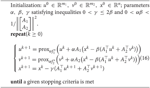
Algorithm 1. Dual Algorithm for Model (1).

3. Parameters Relaxation and Gauss-Seidel Method for Algorithm 1 and Its Convergence Analysis

In this section, Algorithm 1 is modified from two aspects. First, the parameter α will be relaxed such that it is different for updating u^k+1 and v^k+1. Second, the block Gauss-Seidel technique is applied in the sense that the updated result u^k+1 will be immediately used in computing v^k+1. As a consequence, we have a new algorithm, as a variant of Algorithm 1, which is depicted in Algorithm 2.

ALGORITHM 2

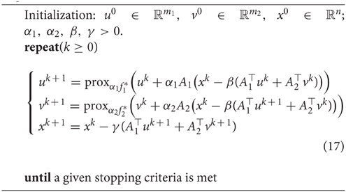
Algorithm 2. Gauss-Seidel Method for Model (1).

Next, we describe the general forms of the schemes (14) and (17) based on which the convergence analysis of the two algorithms will be derived. By the definition of proximity operator, the first step of iterative scheme (14) can be equivalently rephrased as

$\begin{array}{ll}{w}^{k+1}=argmin\left\{\begin{array}{c}{f}^{*}(w)+\frac{1}{2\alpha }||w\hfill \\ -(w^k+\alpha A(x^k-\beta A^{\top }{w}^k))|{|}_2^2:w\in {ℝ}^m\hfill \end{array}\right\}.\hfill & (18)\end{array}$

rearranging the objective function in Equation (18) and ignoring some constant, the optimization problem of Equation (18) is equivalent to

$\begin{array}{ll}\begin{array}{c}{w}^{k+1}=argmin\left\{\begin{array}{c}{f}^{*}(w)-\langle x^k,A^{\top }w\rangle +\frac{\beta }{2}||A^{\top }w|{|}_2^2+\frac{1}{2}\\ \langle (\frac{1}{\alpha }I-\beta A{A}^{\top })(w-w^k),w-w^k\rangle :\hfill \\ w\in {ℝ}^m\hfill \end{array}\right\}.\hfill \end{array}& (19)\end{array}$

Under the condition $0<\alpha \beta <\frac{1}{\left|\right|A|{|}^2}$, where ||A|| is the largest singular value of A, the matrix $\frac{1}{\alpha }I-\beta A{A}^{\top }$ is symmetric, positive definite. As a result, the iterative scheme (14) can be cast into the following iterative scheme given in Zhang et al. [1]:

$\{\begin{array}{l}{w}^{k+1}=\text{argmin }\left\{\begin{array}{l}{f}^{\ast }(w)-\langle x^k,A^{\top }w\rangle +\frac{\beta }{2}\Vert A^{\top }w{\Vert }_2^2\\ +\frac{1}{2}\Vert w-w^k{\Vert }_Q^2:w\in {ℝ}^m\end{array}\right\},\hfill \\ x^{k+1}=x^k-\gamma A^{\top }{w}^{k+1}\hfill & (20)\end{array}$

where the Q−norm || · ||_Q is defined as $\sqrt{\langle Q·,·\rangle }$ for a positive definite symmetric matrix Q.

Similarly, the iterative scheme (17) in Algorithm 2 can be cast as a special case of the following scheme

$\{\begin{array}{l}{u}^{k+1}=\text{argmin}\{f_1^{\ast }(u)-\langle x^k,A_1^{\top }u+A_2^{\top }{v}^k\rangle +\frac{\beta }{2}\Vert A_1^{\top }u\hfill \\ +A_2^{\top }{v}^k{\Vert }_2^2+\frac{1}{2}\Vert u-u^k{\Vert }_{Q_1}^2:u\in {ℝ}^{m_1}\}\hfill \\ v^{k+1}=\text{argmin}\{f_2^{\ast }(v)-\langle x^k,A_1^{\top }{u}^{k+1}+A_2^{\top }v\rangle \text{ ,}\hfill \\ +\frac{\beta }{2}\Vert A_1^{\top }{u}^{k+1}+A_2^{\top }v{\Vert }_2^2+\frac{1}{2}\Vert v-v^k{\Vert }_{Q_2}^2:v\in {ℝ}^{m_2}\}\hfill \\ x^{k+1}=x^k-\gamma (A_1^{\top }{u}^{k+1}+A_2^{\top }{v}^{k+1})\hfill & (21)\end{array}$

where both Q₁ and Q₂ are symmetric and positive definite matrices. Indeed, by choosing $Q_1=\frac{1}{{\alpha }_1}I-\beta A_1{A}_1^{\top },Q_2=\frac{1}{{\alpha }_2}I-\beta A_2{A}_2^{\top }$ with $0<{\alpha }_1\beta <\frac{1}{\left|\right|A_1|{|}^2}$ and $0<{\alpha }_2\beta <\frac{1}{\left|\right|A_2|{|}^2}$, the matrices Q₁, Q₂ are symmetric, positive definite and scheme (21) reduces to (17) in Algorithm 2. Recall that the parameters α, β in Algorithm 1 need satisfy $0<\alpha \beta <\frac{1}{\left|\right|A|{|}^2}$, where A is chosen as Equation (15). It can be noticed that $max\left\{\left|\right|A_1|{|}^2,|\left|A_2\right|{|}^2\right\}\le \left|\right|A|{|}^2$, which implies $min\left\{\frac{1}{\left|\right|A_1|{|}^2},\frac{1}{\left|\right|A_2|{|}^2}\right\}\ge \frac{1}{\left|\right|A|{|}^2}$. Hence, more flexibility exhibits for the choice of α₁, α₂, β in Algorithm 2 than for the choice of α, β in Algorithm 1.

We remark that the iterative scheme (21) generalizes the iterative scheme (22)

$\{\begin{array}{l}{u}^{k+1}=\text{argmin}\{f_1^{\ast }(u)-\langle x^k,A_1^{\top }u-v^k\rangle +\frac{\beta }{2}\Vert A_1^{\top }u-v^k{\Vert }_2^2\hfill \\ +\frac{1}{2}\Vert u-u^k{\Vert }_{Q_1}^2:u\in {ℝ}^{m_1}\}\hfill \\ v^{k+1}=\text{argmin}\{f_2^{\ast }(v)-\langle x^k,A_1^{\top }{u}^{k+1}\hfill \\ -v\rangle +\frac{\beta }{2}\Vert A_1^{\top }{u}^{k+1}-v{\Vert }_2^2+\frac{1}{2}\Vert v-v^k{\Vert }_{Q_2}^2:v\in {ℝ}^{m_2}\}\hfill \\ x^{k+1}=x^k-\gamma (A_1^{\top }{u}^{k+1}-v^{k+1})\hfill & (22)\end{array}$

whose form is equivalent to Equation (6) by specifying the variables, functions and matrices appropriately. Indeed, when A₂ is specified as −I, the iterative scheme (21) reduces to (22). Unlike [1], the iterative scheme (21) is derived from the dual formulation instead of primal problems. In addition, the generality of matrix A₂ in iterative scheme (21) generalizes the matrix −I in scheme (6).

The rest of this section is devoted to a unified convergence analysis of the two iterative schemes (20) and (21), from which Algorithm 1 and Algorithm 2 can be derived. The convergence of these two schemes is analyzed in the following manner: we first prove the convergence of schemes (21) and obtain the convergence of scheme (20) as an immediate result.

For convenient exposition, Equation (9) for the special case Equation (15) is rewritten as

$\begin{array}{ll}{A}_1^{\top }û+A_2^{\top }\widehat{v}=0,A_1\widehat{x}\in \partial f_1^{*}(û),\text{\hspace{1em}and\hspace{1em}}{A}_2\widehat{x}\in \partial f_2^{*}(\widehat{v}).& (23)\end{array}$

We will show that for any initial seed $(u^0,v^0,x^0)\in {ℝ}^{m_1}\times {ℝ}^{m_2}\times {ℝ}^n$ and a positive parameter γ the sequence ({(u^k, v^k, x^k):k ∈ ℕ}) converges to a triple $(û,\widehat{v},\widehat{x})\in {ℝ}^{m_1}\times {ℝ}^{m_2}\times {ℝ}^n$ satisfying Equation (23).

First of all, we look at the characterization of u^k+1, v^k+1 involved in the two subproblems in Equation (21). Using Fermat's rule for the two subproblems, we are able to get

$\{\begin{array}{l}{A}_1{x}^k-\beta A_1(A_1^{\top }{u}^{k+1}+A_2^{\top }{v}^k)-Q_1(u^{k+1}-u^k)\in \partial f_1^{\ast }(u^{k+1}),\hfill \\ A_1{x}^k-\beta A_1(A_1^{\top }{u}^{k+1}+A_2^{\top }{v}^k)-Q_2(u^{k+1}-u^k)\in \partial f_2^{\ast }(v^{k+1})\hfill \end{array}.$

Let

$\{\begin{array}{l}{r}^{k+1}: =A_1{x}^k-\beta A_1(A_1^{\top }{u}^{k+1}+A_2^{\top }{v}^k)-Q_1(u^{k+1}-u^k),\hfill \\ t^{k+1}: =A_2{x}^k-\beta A_2(A_1^{\top }{u}^{k+1}+A_2^{\top }{v}^{k+1})-Q_2(v^{k+1}-v^k)\hfill & .(24)\end{array}$

Then $r^{k+1}\in f_1^{*}(u^{k+1}),t^{k+1}\in f_2^{*}(v^{k+1})$. If the sequence ({(u^k, v^k, x^k) : k ∈ ℕ}) converges to a triple $(û,\widehat{v},\widehat{x})\in {ℝ}^{m_1}\times {ℝ}^{m_2}\times {ℝ}^n$ satisfying Equation (23), we observe $r^{k+1}\to A_1\widehat{x},t^{k+1}\to A_2\widehat{x}$ as k → ∞. For convenience, we also introduce the following notations

$\begin{array}{l}\widehat{\rho }:=\left[\begin{array}{c}\widehat{u}\\ \widehat{v}\\ \widehat{\widehat{x}}\end{array}\right],{\rho }^k:=\left[\begin{array}{c}{u}^k\\ v^k\\ x^k\end{array}\right],P:=\left[\begin{array}{ccc}{Q}_1& & \\ & Q_2& \\ & & \frac{1}{\gamma }I\end{array}\right],r:=A_1\widehat{x},\hfill \\ t:=A_2\widehat{x}\hfill \\ u_e^k:=u^k-\widehat{u},v_e^k:=v^k-\widehat{v},x_e^k:=x^k-\widehat{x},\hfill \\ r_e^{k+1}:=r^{k+1}-r,t_e^{k+1}:=t^{k+1}-t,{\rho }_e^k:={\rho }^k-\widehat{\rho }.\hfill \end{array}$

Next, we shall establish a relationship between a triple $(û,\widehat{v},\widehat{x})$ and the sequence {(u^k, v^k, x^k):k ∈ ℕ} generated by the iterative scheme (21).

Lemma 3.1. Let Q₁ and Q₂ be two positive definite symmetric matrices, let the triple $(û,\widehat{v},\widehat{x})\in {ℝ}^{m_1}\times {ℝ}^{m_2}\times {ℝ}^n$satisfy Equation (23), and let {(u^k, v^k, x^k) : k ∈ ℕ} be the sequence generated by scheme (21).

Then the following equation holds:

$\begin{array}{ll}(||{\rho }_e^{k+1}|{|}_P^2+\beta ||A_2^{\top }{v}_e^{k+1}|{|}^2)-(||{\rho }_e^k|{|}_P^2+\beta ||A_2^{\top }{v}_e^k|{|}^2)=y^k,& (25)\end{array}$

where

$\begin{array}{l}{y}^k=-||u^{k+1}-u^k|{|}_{Q_1}^2-2\langle r_e^{k+1},u_e^{k+1}\rangle -||v^{k+1}-v^k|{|}_{Q_2}^2\hfill \\ -2\langle t_e^{k+1},v_e^{k+1}\rangle -(\beta -\gamma )||A_1^{\top }{u}^{k+1}+A_2^{\top }{v}^{k+1}|{|}^2\hfill \\ -\beta ||A_1^{\top }{u}^{k+1}+A_2^{\top }{v}^k|{|}^2.\hfill \end{array}$

PROOF. It follows from the definitions of r, r^k, t, and t^k, the iteration scheme (21) and the characterization of saddle points Equation (23) that

$\{\begin{array}{l}{r}_e^{k+1}-A_1{x}_e^k+\beta A_1(A_1^{\top }{u}_e^{k+1}+A_2^{\top }{v}_e^k)\hfill \\ +Q_1(u^{k+1}-u^k)=0,\hfill \\ t_e^{k+1}-A_2{x}_e^k+\beta A_2(A_1^{\top }{u}_e^{k+1}+A_2^{\top }{v}_e^{k+1})\hfill \\ +Q_2(v^{k+1}-v^k)=0,\hfill \\ x_e^{k+1}=x_e^k-\gamma (A_1^{\top }{u}_e^{k+1}+A_2^{\top }{v}_e^{k+1}).\hfill & (26)\end{array}$

By taking the inner product with $2u_e^{k+1}$ on the both sides of the first equality of Equation (26) and rearranging the terms and using the identity $\left|\right|u_e^k|{|}_{Q_1}^2=||u^{k+1}-u^k|{|}_{Q_1}^2+\left|\right|u_e^{k+1}|{|}_{Q_1}^2-2\langle Q_1(u^{k+1}-u^k),u_e^{k+1}\rangle$, we obtain

$\begin{array}{l}(||u_e^{k+1}|{|}_{Q_1}^2-||u_e^k|{|}_{Q_1}^2)=-||u^{k+1}-u^k|{|}_{Q_1}^2-2\langle r_e^{k+1},u_e^{k+1}\rangle \\ -2\beta \langle A_1^{\top }{u}_e^{k+1},A_1^{\top }{u}_e^{k+1}+A_2^{\top }{v}_e^k\rangle \\ +2\langle A_1^{\top }{u}_e^{k+1},x_e^k\rangle ,\end{array}$

Likewise, by taking the inner product with $2v_e^{k+1}$ and $2x_e^k$ on the both sides of the second and third Equations of (26), we obtain

$\begin{array}{l}(||v_e^{k+1}|{|}_{Q_2}^2-||v_e^k|{|}_{Q_2}^2)=-||v^{k+1}-v^k|{|}_{Q_2}^2-2\langle t_e^{k+1},v_e^{k+1}\rangle \\ -2\beta \langle A_2^{\top }{v}_e^{k+1},A_1^{\top }{u}_e^{k+1}+A_2^{\top }{v}_e^{k+1}\rangle \\ +2\langle A_2^{\top }{v}_e^{k+1},x_e^k\rangle ,\end{array}$

and

$\begin{array}{l}\frac{1}{\gamma }(||x_e^{k+1}|{|}_2^2-||x_e^k|{|}_2^2)=\gamma ||A_1^{\top }{u}_e^{k+1}+A_2^{\top }{v}_e^{k+1}|{|}^2\\ -2\langle x_e^k,A_1^{\top }{u}_e^{k+1}+A_2^{\top }{v}_e^{k+1}\rangle ,\end{array}$

respectively. By adding up the above three equations and using the identity $\left|\right|{\rho }^k-\widehat{\rho }|{|}_P^2=||u^k-û|{|}_{Q_1}^2+\left|\right|v^k-\widehat{v}|{|}_{Q_2}^2+\frac{1}{\gamma }||x^k-\widehat{x}|{|}_2^2$ and the fact $A_1^{\top }û+A_2^{\top }\widehat{v}=0$, we get Equation (25). This completes the proof of the result.                         □

To show that the convergence of sequence {(u^k, v^k, x^k):k ∈ ℕ} generated by the iterative scheme (21), we need two properties of the subdifferential. The first one is the monotonicity of the subdifferantial. The subdifferential a function $\psi \in {\Gamma }_0({ℝ}^d)$ as a set-valued function is monotone (see [15]) in the sense that for any u and v in the domain of ψ

$\begin{array}{l}\langle \tilde{u}-\tilde{v},u-v\rangle \ge 0,\text{\hspace{1em}for all\hspace{1em}}\tilde{u}\in \partial \psi (u),\tilde{v}\in \partial \psi (v).\end{array}$

Another useful property of the sub-differential is presented in the following lemma.

Lemma 3.2. Let ψ be in ${\Gamma }_0({ℝ}^d)$ and let {(x^k, y^k) : k ∈ ℕ} be a sequence with y^k ∈ ∂ψ(x^k). Suppose that x^k → x and y^k → y as k → ∞. Then y ∈ ∂ψ(x).

PROOF. By the definition of sub-differential, the inequality ψ(z) ≥ ψ(x^k) + 〈y^k, z − x^k〉 holds all z ∈ ℝ^d and k ∈ ℕ. By taking limit inferior to both sides of the above inequality, it follows that $\psi (z)\ge {\text{lim inf}}_{k\to \infty }(\psi (x^k)+\langle y^k,z-x^k\rangle )$. By virtue of the lower semi-continuity of ψ, i.e., ${\text{lim inf}}_{k\to \infty }\psi (x^k)\ge \psi (x)$, and the fact of 〈y^k, z − x^k〉 → 〈y, z − x〉, we obtain that ψ(z) ≥ ψ(x) + 〈y, z − x〉, for all z ∈ ℝ^d. That is, y ∈ ∂ψ(x).                       □

With these preparations, we are ready to prove the convergence of the sequence {(u^k, v^k, x^k) : k ∈ ℕ} generated by the iterative scheme (21).

Theorem 3.3. Let Q₁ and Q₂ be two positive definite symmetric matrices and let {(u^k, v^k, x^k) : k ∈ ℕ} be the sequence generated by scheme (21). If 0 < γ ≤ β, then the sequence {(u^k, v^k, x^k) : k ∈ ℕ} converges to a triple $(û,\widehat{v},\widehat{x})$ satisfying Equation (23).

PROOF. To show {(u^k, v^k, x^k) : k ∈ ℕ} converges to a triple $(û,\widehat{v},\widehat{x})$ satisfying Equation (23), we first show {(u^k, v^k, x^k) : k ∈ ℕ} is bounded and therefore has a convergent subsequence, then show that this convergent subsequence converges to a triple $(û,\widehat{v},\widehat{x})$ satisfying Equation (23) and finally show the entire sequence {(u^k, v^k, x^k) : k ∈ ℕ} converges to this triple $(û,\widehat{v},\widehat{x})$.

Let the symbols ρ, ρ^k, ${\rho }_e^k$, P, r, r^k, $r_e^k$, t, t^k, $t_e^k$, and y^k be the same as before. Equations (23) and (24) and the monotonicity of subdifferential yield

$\begin{array}{ll}\langle r_e^{k+1},u_e^{k+1}\rangle \ge 0\text{\hspace{1em}and\hspace{1em}}\langle t_e^{k+1},v_e^{k+1}\rangle \ge 0.& (27)\end{array}$

Therefore, when 0 < γ ≤ β, the values of y^k are non-positive. Thus, from Equation (25) we know that the sequence $\left\{\left|\right|{\rho }_e^k|{|}_P^2+\beta |\left|A_2^{\top }{v}_e^k\right|{|}_2^2:k\in \mathbb{N}\right\}$ is decreasing and convergent. This implies the boundedness of the sequence $\left\{\left|\right|{\rho }^k-\rho |{|}_P:k\in \mathbb{N}\right\}$ which further yield the boundedness of the sequence {(u^k, v^k, x^k) : k ∈ ℕ}. Therefore, there exists a convergent subsequence $\left\{(u^{k_i},v^{k_i},x^{k_i}):i\in \mathbb{N}\right\}$ such that for some vector $(\tilde{u},\tilde{v},\tilde{x})\in {ℝ}^{m_1}\times {ℝ}^{m_2}\times {ℝ}^n$

$\begin{array}{ll}(u^{k_i},v^{k_i},x^{k_i})\to (\tilde{u},\tilde{v},\tilde{x})& (28)\end{array}$

as i goes to infinity.

We shall show that $(\tilde{u},\tilde{v},\tilde{x})$ satisfies Equation (23), that is, $A_1^{\top }\tilde{u}+A_2^{\top }\tilde{v}=0$, $A_1\tilde{x}\in \partial f_1^{*}(\tilde{u})$, and $A_2\tilde{x}\in \partial f_2^{*}(\tilde{v})$. Summing Equation (25) for k from 1 to infinity, we conclude that

$\begin{array}{l}{\displaystyle \sum _{k=1}^{\infty }(\Vert u^{k+1}-u^k{\Vert }_{Q_1}^2+\Vert v^{k+1}-v^k{\Vert }_{Q_2}^2+(\beta -\gamma )\Vert A_1^{\top }{u}^{k+1}}\hfill \\ +A_2^{\top }{v}^{k+1}{\Vert }_2^2)\le \Vert {\rho }_e^1{\Vert }_P^2+\beta \Vert A_2^{\top }{v}_e^1{\Vert }_2^2.\hfill & (29)\end{array}$

The convergence of three series in inequality Equation (29) yields that as k goes to infinity

$\begin{array}{l}{u}^{k+1}-u^k\to 0,v^{k+1}-v^k\to 0,A_1^{\top }{u}^{k+1}+A_2^{\top }{v}^{k+1}\to 0,\end{array}$

which particularly indicate

$\begin{array}{ll}{u}^{k_i+1}-u^{k_i}\to 0,v^{k_i+1}-v^{k_i}\to 0,A_1^{\top }{u}^{k_i+1}+A_2^{\top }{v}^{k_i+1}\to 0,& (30)\end{array}$

as i goes to infinity. By Equations (28) and (30), we have that

$\begin{array}{ll}{\displaystyle \underset{i\to \infty }{lim}}{u}^{k_i+1}=\tilde{u},{\displaystyle \underset{i\to \infty }{lim}}{v}^{k_i+1}=\tilde{v},& (31)\end{array}$

and

$\begin{array}{ll}{A}_1^{\top }\tilde{u}+A_2^{\top }\tilde{v}={\displaystyle \underset{i\to \infty }{lim}}\left(A_i^{\top }{u}^{k_i+1}+A_2^{\top }{v}^{k_i+1}\right)=0.& (32)\end{array}$

Equations (28), (30) and (32) together with the definitions of r^k and t^k yield

$\begin{array}{ll}{\displaystyle \underset{i\to \infty }{lim}}{r}^{k_i+1}=A_1\tilde{x}\text{\hspace{1em}and\hspace{1em}}{\displaystyle \underset{i\to \infty }{lim}}{t}^{k_i+1}=A_2\tilde{x}.& (33)\end{array}$

Recall that $r^{k_i+1}\in \partial f_1^{*}(u^{k_i+1}),t^{k_i+1}\in \partial f_2^{*}(v^{k_i+1})$ and Equations (31) and (33). We obtain from Lemma 3.2 that $A_1\tilde{x}\in \partial f_1^{*}(\tilde{u})$ and $A_2\tilde{x}\in \partial f_2^{*}(\tilde{v})$. Hence, the vector $(\tilde{u},\tilde{v},\tilde{x})$ satisfies Equation (28).

Now, let us take $(û,\widehat{v},\widehat{x})=(\tilde{u},\tilde{v},\tilde{x})$. Then from Equation (28) we have that

$\begin{array}{l}{\displaystyle \underset{i\to \infty }{lim}}\left(||{\rho }^{k_i}-\widehat{\rho }|{|}_P^2+\beta ||A_2^{\top }(v^{k_i}-\widehat{\widehat{v}})|{|}^2\right)=0.\end{array}$

The monotonicity and convergence of the sequence $\left\{\left|\right|{\rho }^k-\widehat{\rho }|{|}_P^2+\beta |\left|A_2^{\top }(v^k-\widehat{v})\right|{|}_2^2:k\in \mathbb{N}\right\}$ imply that

$\begin{array}{l}{\displaystyle \underset{k\to \infty }{lim}}\left(||{\rho }^k-\widehat{\rho }|{|}_P^2+\beta ||A_2^{\top }(v^k-\widehat{v})|{|}_2^2\right)=0.\end{array}$

Thus, the sequence {(u^k, v^k, x^k) : k ∈ ℕ} converges to $(\tilde{u},\tilde{v},\tilde{x})$ satisfying Equation (23). This completes the proof of this theorem.                   □

Next, we will show that we can specify scheme (20) as a special case of scheme (21) and therefore the convergence of scheme (20) follows automatically. To this end, we consider the two schemes (20), (21) are mutually independent and functions or matrices in the two schemes are not related hereafter.

To cast scheme (20) as scheme (21), we let

$\begin{array}{ll}u=w,f_1^{*}=f^{*},f_2^{*}=0,A_1=A,A_2=0,Q_1=Q& (34)\end{array}$

in scheme (21). For such the choice of those quantities, we are able to rewrite scheme (21) as

$\{\begin{array}{l}{w}^{k+1}=\text{argmin}\{f^{\ast }(w)-\langle x^k,A^{\top }w\rangle +\frac{\beta }{2}\Vert A^{\top }w{\Vert }_2^2\hfill \\ +\frac{1}{2}\Vert u-u^k{\Vert }_Q^2\}\hfill \\ v^{k+1}=\text{argmin}\{-\langle x^k,A^{\top }{w}^{k+1}\rangle +\frac{\beta }{2}\Vert A^{\top }{w}^{k+1}{\Vert }_2^2,\hfill \\ +\frac{1}{2}\Vert v-v^k{\Vert }_{Q_2}^2\}\hfill \\ x^{k+1}=x^k-\gamma (A^{\top }{w}^{k+1})\hfill & (35)\end{array}$

from which one can notice that sequence {v^k : k ∈ ℕ} is a constant vector sequence. Ignoring the trivial step involving v^k+1, scheme (35) becomes scheme (20).

Lemma 3.4. Let Q be a positive definite symmetric matrix, let the pair $(ŵ,\widehat{x})\in {ℝ}^m\times {ℝ}^n$ satisfy Equation (9), and let {(w^k, x^k) : k ∈ ℕ} be the sequence generated by scheme (20). Set

$\begin{array}{l}s:=A\widehat{x},s^{k+1}:=A{x}^k-\beta A{A}^{\top }{w}^{k+1}-Q(w^{k+1}-w^k),\\ \widehat{\rho }:=\left[\begin{array}{c}\widehat{w}\\ \widehat{x}\end{array}\right],{\rho }^k:=\left[\begin{array}{c}{w}^k\\ x^k\end{array}\right],andP:=\left[\begin{array}{cc}Q& \\ & \frac{1}{\gamma }I\end{array}\right].\end{array}$

Then

$\begin{array}{l}||{\rho }^{k+1}-\widehat{\rho }|{|}_P^2-||{\rho }^k-\widehat{\rho }|{|}_P^2=-||w^{k+1}-w^k|{|}_Q\hfill \\ -2\langle s^{k+1}-s,w^{k+1}-ŵ\rangle \hfill \\ -(2\beta -\gamma )||A^{\top }(w^{k+1}-ŵ)|{|}_2^2.\hfill & (36)\end{array}$

PROOF. This is an immediate result of Lemma 3.1 by specifying corresponding quantities as in Equation (34) and noticing that v^k+1 = v^k for such the choice of those quantities.            □

With Lemma 3.4, we can prove our result on the convergence of the sequence {(w^k, x^k) : k ∈ ℕ} generated by scheme (20).

Theorem 3.5. Let Q be a positive definite symmetric matrix and let {(w^k, x^k) : k ∈ ℕ} be the sequence generated by scheme (20). If 0 < γ ≤ 2β then the sequence {(w^k, x^k) : k ∈ ℕ} converges to a pair $(ŵ,\widehat{x})$ satisfying Equation (9).

PROOF. It follows the proof of Theorem 3.3 by specifying corresponding quantities in scheme (21) as in (34) and using Lemma 3.4.                 □

We remark that authors in Zhang et al. [1] only shown convergent subsequence of {(w^k, x^k) : k ∈ ℕ} converges to a pair $(ŵ,\widehat{x})$ satisfying Equation (9). But as shown by Theorem 3.5, the entire sequence {(w^k, x^k) : k ∈ ℕ} converges to the same point, which strengthens the result in Zhang et al. [1].

4. Connections to Existing Algorithms

In this section, we point out the connections of our proposed algorithms to several well-known methods. Specifically, we would explore the connection of the proposed algorithms to Chambolle and Pock's Primal-Dual method, Augmented Lagrangian Method, Alternating Direction Method of Multipliers, and Generalized ADM.

4.1. Connection to Chambolle and Pock's Algorithm

First of all, let us review Chambolle and Pock's (CP) method [9] for solving the following optimization problem

$\begin{array}{ll}min\left\{f(Ax)+g(x):x\in {ℝ}^n\right\},& (37)\end{array}$

where $f\in {\Gamma }_0({ℝ}^m)$, $g\in {\Gamma }_0({ℝ}^n)$, and A is a matrix of size m × n. We assume that model (37) has a minimizer. The CP method proposed in Chambolle and Pock [9] for model (37) can be written as

$\{\begin{array}{l}{w}^{k+1}={\text{prox}}_{\sigma f^{\ast }}(w^k+\sigma A{\overline{x}}^k),\hfill \\ x^{k+1}={\text{prox}}_{\tau g}(x^k-\tau A^{\top }{w}^{k+1}),\hfill \\ {\overline{x}}^{k+1}=2x^{k+1}-x^k.\hfill & (38)\end{array}$

For any initial guess $(x^0,{\stackrel{-}{x}}^0,w^0)\in {ℝ}^n\times {ℝ}^n\times {ℝ}^m$, the sequence {(x^k, w^k) : k ∈ ℕ} converges as long as 0 < στ < ||A||⁻².

In particular, when we set g = 0, a direct computation shows that prox_τg is the identity operator for any τ > 0. Set α = σ and β = 2τ. Accordingly, the general CP method in Equation (38) becomes

$\{\begin{array}{l}{w}^{k+1}={\text{prox}}_{\alpha f^{\ast }}\left(w^k+\alpha A\left(x^{k-1}-\beta A^{\top }{w}^k\right)\right),\hfill \\ x^{k+1}=x^k-\frac{\beta }{2}{A}^{\top }{w}^{k+1}.\hfill & (39)\end{array}$

On the other hand, when we set g = 0, model (37) reduces to model (3). Our algorithm for model (3) is presented in scheme (14).

Therefore, by comparing the CP method and the scheme (14) for model (3), we can see that the CP method uses x^k−1 while the scheme (14) uses x^k in the computation of w^k+1. Further, the step size of the CP method for updating x^k+1 is fixed as $\frac{\beta }{2}$ while it can be any number in (0, 2β] for the scheme (14). Although, the relation 0 < αβ < 2||A||⁻² is required for the CP method while the relation 0 < αβ < ||A||⁻² is needed for the scheme (14), for a fixed α, we can choose the step size for the scheme (14) twice bigger than that for the CP method.

4.2. Connection to Augmented Lagrangian Methods

As we already know that the scheme (14) model (3) is derived from the scheme (20) with a proper chosen Q. The scheme (20) is used to solve the constrained dual optimization problem (7).

In the literature of nonlinear programming [16], augmented Lagrangian methods (ALMs) are often used to convert a constrained optimization problem to an unconstrained one by adding the objective function a penalty term associated with the constraints. For model (7), the augmented Lagrangian method is as follows:

$\{\begin{array}{l}{w}^{k+1}=\text{argmin}\{f^{\ast }(w)-\langle x^k,A^{\top }w\rangle +\frac{\beta }{2}\Vert A^{\top }w{\Vert }_2^2:w\in {ℝ}^m\},\\ x^{k+1}=x^k-\beta A^{\top }{w}^{k+1}.& (40)\end{array}$

We can see that the scheme (20) reduces to the ALM Equation (40) if we choose Q = 0 and γ = β in Equation (20). Even though we can assume that the proximity operator of f has a closed form, there is lack of an effective way to update w^k+1 in Equation (40) when A is not the identity matrix. However, the vector w^k+1 in the scheme (20) can be effectively updated once a proper Q is chosen. This essentially illustrates that Algorithm 1 is superior to the ALM from the numerical implementation point of view.

4.3. Connection to Alternating Direction Method of Multipliers

By specializing the dual formulation (7) of model (7) to model (1), we have that

$\begin{array}{ll}min\left\{{\displaystyle f_1^{*}}(u)+f_2^{*}(v):A_1^{\top }u+A_2^{\top }v=0,u\in {ℝ}^{m_1},v\in {ℝ}^{m_2}\right\}.& (41)\end{array}$

The alternating direction method of multipliers (ADMM) for dual problem (41) reads as

$\{\begin{array}{l}{u}^{k+1}=\text{argmin}\{f_1^{\ast }(u)+f_2^{\ast }(v^k)-\langle x^k,A_1^{\top }u+A_2^{\top }{v}^k\rangle \hfill \\ +\frac{\beta }{2}\Vert A_1^{\top }u+A_2^{\top }{v}^k{\Vert }_2^2:u\in {ℝ}^{m_1}\}\hfill \\ v^{k+1}=\text{argmin}\{f_1^{\ast }(u^{k+1})+f_2^{\ast }(v)-\langle x^k,A_1^{\top }{u}^{k+1}+A_2^{\top }v\rangle .\hfill \\ +\frac{\beta }{2}\Vert A_1^{\top }{u}^{k+1}+A_2^{\top }v{\Vert }_2^2:v\in {ℝ}^{m_2}\}\hfill \\ x^{k+1}=x^k-\beta (A_1^{\top }{u}^{k+1}+A_2^{\top }{v}^{k+1})\hfill & (42)\end{array}$

We can see that the scheme (21) reduces to the above ADMM method if we set Q₁ = 0, Q₂ = 0, and γ = β in Equation (21). Similar to what we have observed for the ALM method, solving the two optimization problems in Equation (42) is still challenging in general when both A₁ and A₂ are not the identity matrix. However, the vectors u^k+1 and v^k+1 in the scheme (21) can be effectively updated once Q₁ and Q₂ are properly chosen. Hence our Algorithm 2 is superior to the ADMM from the numerical implementation point of view.

4.4. Connection to Generalized Alternating Direction Method

Finally, we comment that the generalized ADM proposed in Deng and Yin [3] can be applied for solving the optimization problem (41) and the resulting algorithm is exactly the same as Algorithm 2. However, the motivations behind [3] and our current paper are completely different. The generalized ADM in Deng and Yin [3] was developed based on the augmented Lagrangian function of the objective function of Equation (41) and the work in there focused on linear convergence rate of the corresponding algorithm. In our current work, we formulated the optimization problem (8) as a constrained optimization problem (8) and recognized the solution of Equation (8) as a solution of a fixed-point equation (see Proposition 2.2) from which Algorithm 2 was naturally derived.

5. Applications to Image Deblurring

In this section, we first identity two well-known image deblurring models, namely L2-TV and L1-TV, as special cases of the general model (1). We then give details on how Algorithms 1 and 2 are applied. In particular, we present the explicit expressions of the proximity operators of $f_1^{*}$ and $f_2^{*}$. Since the total variation (TV) is involved in the both image deblurring models, we begin with presenting the discrete setting for total variation.

For convenience of exposition, we assume that an image considered in this paper has a size of $\sqrt{n}\times \sqrt{n}$. The image is treated as a vector in ℝⁿ in such a way that the ij-th pixel of the image corresponds to the $(i+(j-1)\sqrt{n})$-th component of the vector in ℝⁿ. The total variation of the image x can be expressed as the composite function of a convex function ψ : ℝ²ⁿ → ℝ and a 2n × n matrix B. To define the matrix B, we need a $\sqrt{n}\times \sqrt{n}$ difference matrix D as follows:

$D:=\left[\begin{array}{cccc}0& & & \\ -1& 1& & \\ & \ddots & \ddots & \\ & & -1& 1\end{array}\right].$

The matrix D will be used to “differentiate” a row or a column of an image matrix. Through the matrix Kronecker product ⊗, we define the 2n × n matrix B by

$\begin{array}{ll}B:=[\begin{array}{c}I\otimes D\\ D\otimes I\end{array}],& (43)\end{array}$

where I is the $\sqrt{n}\times \sqrt{n}$ identity matrix. The matrix B will be used to “differentiate” the entire image matrix. The norm of B is $\left|\right|B|{|}^2=8{sin}^2\frac{(\sqrt{n}-1)\pi }{2\sqrt{n}}$ (see [17]).

We define ψ : ℝ²ⁿ → ℝ is at y ∈ ℝ²ⁿ as

$\begin{array}{ll}\psi (y):={\displaystyle \sum _{i=1}^n}\left|\right|{\left[y_i,y_{n+i}\right]}^{\top }|{|}_2,& (44)\end{array}$

Based on the definition of the 2n × n matrix B and the convex function ψ, the total variation of an image x can be denoted by ψ(Bx) for (isotropic) total variation, i.e.,

$\begin{array}{ll}||x|{|}_{TV}: =\psi (Bx).& (45)\end{array}$

5.1. The L2-TV Image Deblurring Model

The L2-TV image deblurring model is usually used for the recovery of an unknown image x ∈ ℝⁿ from an observable data b ∈ ℝⁿ modeled by

$\begin{array}{ll}b=Kx+\mathrm{\text{white noise}}& (46)\end{array}$

where K is a blurring matrix of size n × n. The L2-TV image deblurring model has the form of

$\begin{array}{ll}\text{min}\left\{\frac{1}{2}\Vert Kx-b{\Vert }_2^2+\mu \Vert x{\Vert }_{\text{TV}}:x\in {ℝ}^n\right\},& (47)\end{array}$

where μ is a regularization parameter.

Now, let us set

$\begin{array}{l}{m}_1=n,m_2=2n,f_1:=\frac{1}{2}||·-b|{|}_2^2,f_2:=\mu \psi ,\hfill \\ A_1:=K,\text{\hspace{1em}and\hspace{1em}}{A}_2:=B,\hfill \end{array}$

where K and b are from Equation (46), ψ is given by Equation (44), and B is defined by Equation (43). Then the L2-TV image deblurring mode (47) can be viewed as a special case of model (1). Therefore, both Algorithms 1 and 2 can be applied for the L2-TV model. Further, we give the explicit forms of the proximity operators ${prox}_{\alpha f_1^{*}}$ and ${prox}_{\alpha f_2^{*}}$ for any positive number α. Actually, using Moreau decomposition and the definition of the proximity operator, we have that for $u\in {ℝ}^{m_1}$

$\begin{array}{l}{prox}_{\alpha f_1^{*}}(u)=\frac{1}{1+\alpha }u-\frac{\alpha }{1+\alpha }b.\end{array}$

For $v\in {ℝ}^{m_2}$, we write $z={prox}_{\alpha f_2^{*}}(v)$. Then for i = 1, 2, …, n, we have that

$\begin{array}{ll}\left[z_i,z_{n+i}\right]=min\left\{||\left[v_i,v_{n+i}\right]|{|}_2,\alpha \right\}\frac{\left[v_i,v_{n+i}\right]}{||\left[v_i,v_{n+i}\right]|{|}_2}.& (48)\end{array}$

5.2. The L1-TV Image Deblurring Model

The L1-TV image deblurring model is usually used for the recovery of an unknown image x ∈ ℝⁿ from an impulsive noise corrupted observable data b ∈ ℝⁿ modeled by

$b_i=\{\begin{array}{ll}0,\hfill & \text{with a probability }p/2;\hfill \\ 255,\hfill & \text{with a probability }p/2;\hfill \\ {(Kx)}_i,\hfill & \text{with a probability }1-p.\hfill & (49)\end{array}$

where K is a blurring matrix of size n × n, p is the noise level, and the index i runs from 1 to n. The L1-TV image deblurring model has the form of

$\begin{array}{ll}min\left\{||Kx-b|{|}_1+\mu ||x|{|}_{TV}:x\in {ℝ}^n\right\},& (50)\end{array}$

where μ is again the regularization parameter.

Now, let us set

$\begin{array}{l}{m}_1=n,m_2=2n,f_1:=||·-b|{|}_1,f_2:=\mu \psi ,\hfill \\ A_1:=K,\text{\hspace{1em}and\hspace{1em}}{A}_2:=B,\hfill \end{array}$

where K and b are from Equation (49), ψ is given by Equation (44), and B is defined by Equation (43). Then the L1-TV image deblurring mode Equation (50) can be viewed as a special case of model (1). Therefore, both Algorithms 1 and 2 can be applied for the L1-TV model. Further, the proximity operator ${prox}_{\alpha f_2^{*}}$ has been given via Equation (48). We jus need to present the proximity operator ${prox}_{\alpha f_1^{*}}$. Actually, we have that for $u\in {ℝ}^{m_1}$

${({\text{prox}}_{\alpha f_1^{\ast }}(u))}_i=\{\begin{array}{ll}\text{sign}(u_i-\alpha b_i),\hfill & \text{if}|u_i-\alpha b_i|\ge 1;\hfill \\ u_i-\alpha b_i,\hfill & \text{otherwise,}\hfill \end{array}$

where i = 1, 2, …, n.

In summary, for both the L2-TV and L1-TV image deblurring models, the associated proximity operators ${prox}_{\alpha f_1^{*}}$ and ${prox}_{\alpha f_2^{*}}$ have closed forms. As a consequence, the sequence {(u^k, v^k, x^k) : k ∈ ℕ} generated by Algorithms 1 and 2 can be efficiently computed.

6. Numerical Experiments

In this section, numerical experiments for image deblurring are carried out to demonstrate the performance of our proposed Algorithms 1 and 2 for the 256 × 256 test images “Cameraman,” “Peppers,” “Goldhill,” and 512 × 512 test image “Lena.” The Chambolle-Pock (CP) algorithm and scheme (6) are compared to our algorithms for the L2-TV and L1-TV image deblurring models. In the following, we quote scheme (6) as ZBO algorithm. Each algorithm is carried out until the stopping criterion ||x^k+1 − x^k||²/||x^k||² ≤ Tol is satisfied, where Tol representing the tolerance, is chosen to be 10⁻⁶. The quality of the recovered images from each algorithm is evaluated by the peak-signal- to-noise ratio (PSNR), which is defined as $PSNR: =20{log}_{10}\frac{255n}{\left|\right|\tilde{x}-x|{|}_2}$, where x ∈ ℝⁿ is the original image and $\tilde{x}$ represents the recovered image. The evolution curve of the function values with respect to iteration will be also adopted to evaluate the performance of algorithms.

In our simulations, blurring matrices K in models (46) and (49) are generated by a rotationally symmetric Gaussian lowpass filter of size “hsize” with standard deviation “sigma” from the MATLAB script fspecial('gaussian', hsize, sigma). Such matrix K is referred to as the (hsize, sigma)-GBM. We remark that the norm of K is always 1, i.e.,

$\begin{array}{ll}||K||=1.& (51)\end{array}$

The (15, 10)-GBM and (21, 10)-GBM are used to generate blurred images in our experiments. All experiments are performed in Matlab 7.11 on Dell Desktop Inspiron 620 with Intel Core i3 CPU @3.30G, 4GB RAM on Windows 7 Home Premium operating system.

6.1. Parameter Settings

Prior to applying Algorithms 1 and 2, and the CP method to the L2-TV model and the L1-TV model for image deblurring problems blurred by (hsize, sigma)-GBMs, the parameters arising from these algorithms need to be determined. Convergence analysis of the algorithms specifies the relation between these parameters. Therefore, once one parameter is fixed, the others can be described by this fixed one. To this end, we fix the value of the parameter β in each above algorithm and then figure out the values of the others.

Let K be a rotationally symmetric Gaussian lowpass filter generated blurring matrix in the L2-TV model and the L1-TV model and let B be the difference matrix defined by Equation (43). We know that ||K|| = 1 by Equation (51) and $\left|\right|B\left|\right|<\sqrt{8}$. To compute the pixel values under the operation of K and B near the boundary of images, we choose to use “symmetric” type for the boundary extension. Correspondingly, we can compute that ${\Vert \left[\begin{array}{c}K\\ B\end{array}\right]\Vert }^2<8$

For Algorithm 1, we set the parameters α and γ as follows:

$\begin{array}{l}\alpha : =\frac{1}{8\beta }\text{\hspace{1em}and\hspace{1em}}\gamma : =2\beta .(52)\end{array}$

For Algorithm 2, we set the parameters α₁, α₂, and γ as follows:

$\begin{array}{ll}{\alpha }_1: =\frac{0.999}{\beta },{\alpha }_2: =\frac{1}{8\beta },\text{\hspace{1em}and\hspace{1em}}\gamma : =\beta .& (53)\end{array}$

For the CP method (see Equation 39), we set

$\begin{array}{ll}\alpha : =\frac{1}{4\beta }.& (54)\end{array}$

With the choices of the parameters given for the algorithms, the convergence of Algorithm 1, Algorithm 2, and the CP method are guaranteed by Theorem 3.5, Theorem 3.3, and a result from Chambolle and Pock [9], respectively. The parameter β in each algorithm is chosen in a way that it would produce better recovered images in terms of PSNR value with the given stopping criterion.

An additional set of parameters for Algorithm 2 will be used as well. They are

$\begin{array}{ll}{\alpha }_1: =\frac{0.999}{\beta },{\alpha }_2: =\frac{1}{8\beta },\text{\hspace{1em}and\hspace{1em}}\gamma : =2\beta .& (55)\end{array}$

By comparing these parameters with those in Equation (53), the parameters α₁ and α₂ are kept unchanged, but the parameter γ in Equation (55) is twice bigger than that in Equation (53). By Theorem 3.3, although the convergence analysis for Algorithm 2 with the parameters given by Equation (55) is missing currently, our numerical experiments presented in the rest of the paper indicate that Algorithm 2 converges and usually produces better recovered images than that with the parameters given by Equation (53) in terms of the CPU times consumed.

6.2. Numerical Results for the L2-TV Image Deblurring

In problems of image deblurring with the L2-TV model, a noisy image is obtained by blurring an ideal image with a (hsize, sigma)-GBM followed by adding white Gaussian noise. Two blurring matrices, namely (21, 10)-GBM and (15, 10)-GBM, are used in our experiments.

For the blurring matrix (21, 10)-GBM, the white noise with mean zero and the standard deviation 1 is added to blurred images. We set the regularization parameter μ = 0.02 in the L2-TV model (47). We choose β = 50 for Algorithm 2, β = 25 for Algorithm 1, β = 50 for the CP method, and β = 0.005 for ZBO method. With these settings, numerical results for four test images “Cameraman,” “Lena,” “Peppers,” and “Goldhill” are reported in Table 1 in terms of numbers of iterations, the CPU times, and the PSNR values. The evolutions of function values for the images of “Peppers” and “Lena” with the L2-TV model are shown in Figure 1. The corresponding curves for the images of “Peppers,” and “Goldhill” are similar to that of “Peppers,” therefore are omitted here. As shown in the Table, Algorithm 2 performs best in terms of computational cost (total iterations and CPU time) and PSNR. Also, as shown in Figure 1 the sequence of function values generated by Algorithm 2 approaches the minimum value fastest, followed by sequences from Algorithm 1 and then by that from CP and ZBO. For the two versions of Algorithm 2, the one with Equation (55) performs slightly better in terms of computational cost and PSNR. The performance of CP and ZBO methods is quite similar in terms of iterations, CPU time, PSNR and evolution of function values. Indeed, the iterations and PSNR in Table 1 are consistent for CP and ZBO methods and the evolution curves of function values for CP and ZBO methods overlap together. We comment that comparable PSNRs and function value can be achieved in Algorithm 1, CP method and ZBO method as in Algorithm 2 if more iteration or computational time is allowed.

TABLE 1

Table 1. Numerical results for the L2-TV model for images blurred by the (21, 10)-GBM.

FIGURE 1

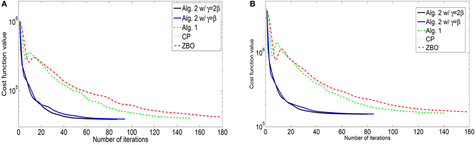
Figure 1. Evolutions of function values of the L2-TV model for images of (A) “Cameraman” and (B) “Lena”.

For the blurring matrix (15, 10)-GBM, the white noise with mean zero and the standard deviation 5 is added to blurred images. We set the regularization parameter μ = 0.2 in the L2-TV model (47). We choose β = 10 for Algorithm 2, β = 5 for Algorithm 1, β = 10 for the CP method, and β = 0.025 for ZBO method. With these settings, numerical results for four test images are reported in Table 2 in terms of numbers of iterations, the CPU times, and the PSNR values. For each image, the PSNR values from each algorithm are comparable. But Algorithm 2 performs better than Algorithm 1, CP and ZBO in terms of computational cost. The evolutions of function values for the images of “Peppers” and “Lena” are shown in Figure 2. The sequence of function values from Algorithm 2 approaches faster to the minimum function value than that from CP and ZBO method. The performance of the two versions of Algorithm 2 is similar. Like in the setting (21, 10)-GBM, the performance of CP and ZBO methods is similar.

TABLE 2

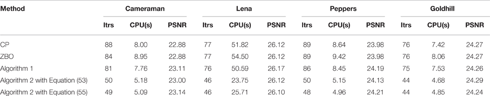
Table 2. Numerical results for the L2-TV model for images blurred by the (15, 10)-GBM.

FIGURE 2

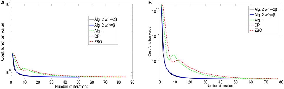
Figure 2. Evolutions of function values of the L2-TV model for images of (A) “Cameraman” and (B) “Lena”.

6.3. Numerical Results for The L1-TV Image Deblurring

In problems of image deblurring with the L1-TV model, a noisy image is obtained by blurring an ideal image with a (hsize, sigma)-GBM followed by adding impulsive noise. Two blurring matrices, namely (21, 10)-GBM and (15, 10)-GBM, are used again in our experiments.

For the blurring matrix (21, 10)-GBM, the impulsive noise with noise level p = 0.3 is added to blurred images. We set the regularization parameter μ = 0.01 in the L1-TV model (50). we set β = 100 for Algorithm 2, β = 50 for Algorithm 1, β = 100 for the CP method, and β = 0.0025 for ZBO method. With these settings, numerical results for four test images “Cameraman,” “Lena,” “Peppers,” and “Goldhill” are reported in Table 3 in terms of numbers of iterations, the CPU times, and the PSNR values. Algorithm 2 yields higher PSNR value but consumes less CPU time than Algorithm 1, CP and ZBO methods. The evolution curves of function values with respect to iteration for the images of “Cameraman” and “Lena” are shown in Figure 3. It can be noticed that sequence of function values generated by Algorithm 2 approaches the minimum value fastest. Regarding the two version of Algorithm 2, the one with setting Equation (55) performs better. We point out that the evolution curves for CP and ZBO overlap with each other. Further, visual quality of the deblurred images of “Cameraman” and “Lena” is shown in Figure 4 for each algorithm. The visual improvement by Algorithm 2 over CP and the ZBO can be seen by the deblurred images.

TABLE 3

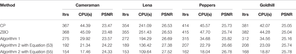
Table 3. Numerical results for the L1-TV model for images blurred by the (21, 10)-GBM.

FIGURE 3

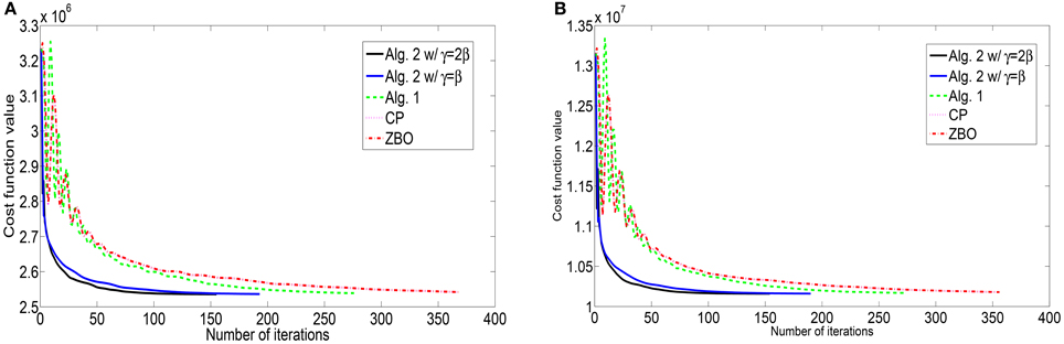
Figure 3. Evolutions of function values of the L1-TV model for images of (A) “Cameraman” and (B) “Lena”.

FIGURE 4

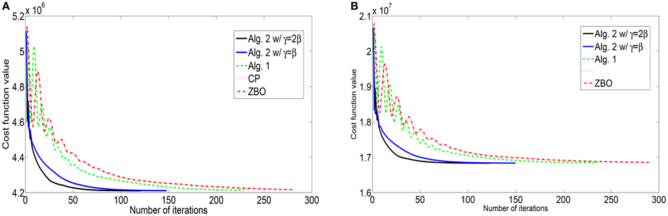
Figure 4. Evolutions of function values of the L1-TV model for images of (A) “Cameraman” and (B) “Lena”.

For the blurring matrix (15, 10)-GBM, the impulsive noise with noise level p = 0.5 is added to blurred images. We set the regularization parameter μ = 0.02 in the L1-TV model (50). we set β = 50 for Algorithm 2, β = 25 for Algorithm 1, β = 50 for the CP method, and β = 0.005 for ZBO method. With these settings, numerical results for four test images “Cameraman,” “Lena,” “Peppers,” and “Goldhill” are reported in Table 4 in terms of numbers of iterations, the CPU times, and the PSNR values. The evolution curves of function values with respect to iteration for the images of “Cameraman” and “Lena” are shown in Figure 5. Visual quality of the deblurred “Cameraman” and “Lena” images is shown in Figure 6 for each algorithm. It is the same as above that Algorithm 2 performs the best.

TABLE 4

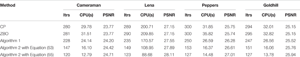
Table 4. Numerical results for the L1-TV model for images blurred by the (15, 10)-GBM.

FIGURE 5

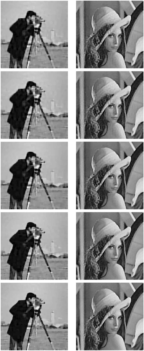
Figure 5. Recovered images of “Cameraman” and “Lena” (from top row to bottom row) with the L1-TV model for images blurred by the (21, 10)-GBM and corrupted by impulsive noise of level p = 0.3. Row 1: the CP; Row 2: ZBO; Row 3: Algorithm 1; Row 4: Algorithm 2 with Equation (53); Row 5: Algorithm 2 with Equation (55).

FIGURE 6

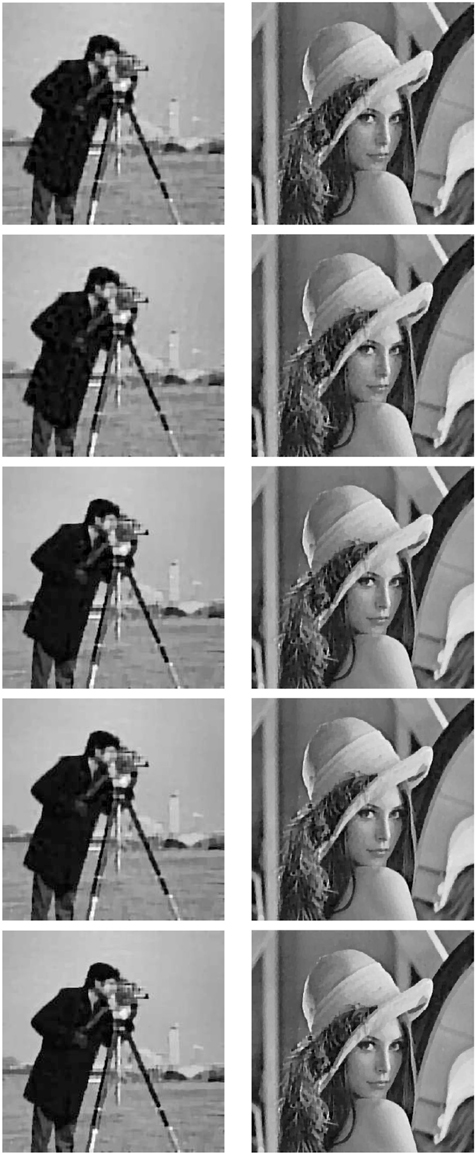
Figure 6. Recovered images of “Cameraman” and “Lena” (from top row to bottom row) with the L1-TV model for images blurred by the (15, 10)-GBM and corrupted by impulsive noise of level p = 0.5. Row 1: the CP; Row 2: the ZBO; Row 3: Algorithm 1; Row 4: Algorithm 2 with Equation (53); Row 5: Algorithm 2 with Equation (55).

7. Conclusion

We propose algorithms to solve a general problem that includes L2-TV and L1-TV image deblurring problems. Algorithm with Block Gauss-Seidel acceleration is also derived for the two term composite minimization Equation (1). The key feature of the proposed algorithms is their ability to yield closed form in each step of iterations. Convergence analysis of the proposed algorithms can be guaranteed under appropriate conditions. Numerical experiments show that the proposed algorithms has computational advantage over CP method and ZBO algorithm.

Author Contributions

All authors listed, have made substantial, direct and intellectual contribution to the work, and approved it for publication.

Funding

The research was supported by the US National Science Foundation under grant DMS-1522332.

Disclaimer

Any opinions, findings and conclusions or recommendations expressed in this material are those of the author(s) and do not necessarily reflect the views of AFRL.

Conflict of Interest Statement

The authors declare that the research was conducted in the absence of any commercial or financial relationships that could be construed as a potential conflict of interest.

References

1. Zhang X, Burger M, Osher S. A unified primal-dual algorithm framework based on Bregman iteration. J Sci Comput. (2011) 46:20–46. doi: 10.1007/s10915-010-9408-8

CrossRef Full Text | Google Scholar

2. Chen P, Huang J, Zhang X. A primal-dual fixed point algorithm for convex separable minimization with applications to image restoration. Inverse Problems (2013) 29:025011. doi: 10.1088/0266-5611/29/2/025011

CrossRef Full Text | Google Scholar

3. Deng W, Yin W. On the global and linear convergence of the generalized alternating direction method of multipliers. J Sci Comput. (2016) 66:889–916. doi: 10.1007/s10915-015-0048-x

CrossRef Full Text | Google Scholar

4. Gabay D, Mercier B. A dual algorithm for the solution of nonlinear variational problems via finite-element approximations. Comput Math Appl. (1976) 2:17–40. doi: 10.1016/0898-1221(76)90003-1

CrossRef Full Text | Google Scholar

5. Glonwinski R, Tallec PL. Augumented Lagrangians and Operator Splitting Methods in Nonlinear Mechanics. Philadephia, PA: SIAM (1989). doi: 10.1137/1.9781611970838

CrossRef Full Text | Google Scholar

6. Hestenes MR. Multiplier and gradient methods. J Optim Theory Appl. (1969) 4:303–20. doi: 10.1007/BF00927673

CrossRef Full Text | Google Scholar

7. Powell MJD. A method for nonlinear constraints in minimization problems. In: Fletcher R, editor, Optimization. New York, NY: Academic Press (1969). p. 283–98.

Google Scholar

8. Rockafeller RT. The multiplier method of Hestenes and Powell applied to convex programming. J Optim Theory Appl. (1973) 12:555–62. doi: 10.1007/BF00934777

CrossRef Full Text | Google Scholar

9. Chambolle A, Pock T. A first-order primal-dual algorithm for convex problems with applications to imaging. J Mat Imaging Vision (2011) 40:120–45. doi: 10.1007/s10851-010-0251-1

CrossRef Full Text | Google Scholar

10. Rockafellar RT, Wets R-JB. Variational Analysis. New York, NY: Springer (1998).

Google Scholar

11. Arrow KJ, Harwicz L, Uzawa H. Studies in Linear and Non-linear Programming. Stanford Mathematical Studies in the Social Science, II. Stanford, CA: Stanford University Press (1958).

12. Esser E, Zhang X, Chan TF. A general framework for a class of first order primal-dual algorithms for convex optimization in imaging science. SIAM J Imaging Sci. (2010) 3:1015–46. doi: 10.1137/09076934X

CrossRef Full Text | Google Scholar

13. Moreau JJ. Fonctions convexes duales et points proximaux dans un espace hilbertien. CR Acad Sci Paris Sér A Math. (1962) 255:1897–2899.

14. Moreau JJ. Proximité et dualité dans un espace hilbertien. Bull Soc Math France (1965) 93:273–99.

Google Scholar

15. Rockafellar RT. Convex Analysis. Princeton, NJ: Princeton University Press (1970).

Google Scholar

16. Bertsekas D. Nonlinear Programming. Belmont, MA: Athena Scientific (2003).

Google Scholar

17. Micchelli CA, Shen L, Xu Y. Proximity algorithms for image models: denoising. Inverse Problems (2011) 27:30. doi: 10.1088/0266-5611/27/4/045009

CrossRef Full Text | Google Scholar