A Review of R-packages for Random-Intercept Probit Regression in Small Clusters

1. Introduction

In behavioral and social sciences, researchers are frequently confronted with clustered or correlated data structures. Such hierarchical data sets for example arise from educational studies, in which students are measured within classrooms, or from longitudinal studies, in which measurements are repeatedly taken within individuals. In these examples, two levels can be distinguished within the data: measurements or level-1 units (e.g., students or time points), and clusters or level-2 units (e.g., classes or individuals). These lower level units are correlated, as outcome measures arising from students with the same teacher, or measurements within an individual, will be more alike than data arising from students with different teachers, or measurements from different individuals. As such, an analysis that ignores these dependencies may yield underestimated standard errors, while inappropriate aggregation across levels may result in biased coefficients [1, 2].

Over the course of decades, several frameworks that can deal with such lower-level correlation have been developed. One such framework entails mixed effect models, which model both the ordinary regression parameters common to all clusters (i.e., the fixed effects), as well as any cluster-specific parameters (i.e., the random effects). Using a parametric approach, two different types can be distinguished: Linear Mixed Models (LMMs) when the outcome is normally distributed, and Generalized Linear Mixed Models (GLMMs) when it is not. A second framework that allows the analysis of multilevel outcomes consists of Structural Equation Models (SEM). Structural Equation Models can be split up into two main classes: “classic” SEM, which is restricted to balanced data, and multilevel SEM, which is able to deal with unbalanced data structures by relying on likelihood-based or Bayesian approaches. Generally, SEM supersects its GLMM counterpart, as the former is able to additionally include latent measures (and measurement error) and assess mediation, in one big model. Discounting these two assets, however, recent literature proves that SEM is completely equivalent to its GLMM counterpart when considering balanced data (e.g., when considering equal cluster sizes in a random intercept model) [3–5].

As clustered Gaussian outcomes have already been discussed thoroughly in the LMM and SEM literature [4–10], we will focus on GLMM- and SEM-methods for non-normal outcome data. More specifically, we will target binary data from small clusters, with a particular focus on clusters of size two, as such settings have proven difficult for the available GLMM methodologies [11, 12]. Clusters of size two are frequently encountered in practice, e.g., when studying dyads [13], in ophthalmology data [14], in twin studies [15], or when analyzing measurements from a 2-period - 2-treatment crossover study [16].

Focusing on the two aforementioned frameworks, current literature on the analysis of clustered binary outcomes reveals two major limitations: clusters of size two were either not considered [17–20], or they were, but limited to only one of both frameworks [21–24]. Here, we compare several estimation procedures within both GLMM- and SEM-frameworks for modeling this type of data, by considering the performance of relevant R-packages. By limiting our comparison to implementations from the statistical environment R (version 3.2.3., [25]), we rely on estimation techniques that are easily accessible to all practitioners (this software is freely available, while at the same time enjoying a wide range of open-source packages). Additionally, we choose to only focus on R-packages which stand on themselves and are not dependent on external software. We do, however, check several of the R-based implementations against others such as implementations in SAS^® software (version 9.4 [26])¹, the MPLUS^® program (version 7 [27]) or the JAGS implementation (version 4.1.0. [28]), as to verify the independence of conclusions on the software used.

In the following sections, we first introduce a motivating example. After this we elaborate on the GLMM and SEM frameworks in general, so that the various estimation methods capable of analyzing the example can be enumerated. Next, we illustrate these methods on our example data. To facilitate the practitioner's decision on which method is most appropriate in which setting, we subsequently conduct a simulation study. Based on our findings we provide recommendations, and end with a discussion.

2. An Example

As a motivating example, we consider data from a randomized study executed by Vandeweghe et al., in preparation in two Flemish nursery schools. As healthy eating habits are important to achieve healthy growth and development in young children, Vandeweghe et al., in preparation focus on strategies to improve the liking of vegetables in preschool children: a child given a tangible or non-tangible reward after tasting should be motivated to taste again. To this end, Vandeweghe et al., in preparation incorporated four possible intervention plans: encouragement toward eating chicory, an active reward after consumption, repeated exposure of the vegetable, and a control group. The binary variable “vegetable liking” (like/ok vs. dislike) was measured during three phases: once during a pre-test (to test their inherent liking of chicory), once during a post-test, and once during a follow-up test. When we only consider the pre- and post-test, we end up with two measurements for each child, while additionally including the follow-up measurements will increase this number to three. So irrespective of whether or not the follow-up measurement is included, the authors end up with a small cluster size.

For illustrative purposes, we will only consider the results from a single school, so that the data structure simplifies to a simple two-level setting where a binary outcome is assessed repeatedly within within each child. Additionally, we will only contrast the “encouragement” vs. the “control” group, as to simplify interpretation and results. The sample size of this reduced data set consists of 37 children (only retaining the complete cases), of which 21 were assigned to the control group and 16 to the encouragement group.

To test whether encouragement increases the liking of chicory, we consider the following random-intercept probit regression model:

$\begin{array}{cc}P(y_{ij}=1\mid x_{ij},b_j)=\Phi ({\beta }_0+{\beta }_1{x}_{ij}+b_j)& \left(1\right)\end{array}$

with index i referring to the measurement moment (i = 0, 1 or 2 for pre-, post- and follow-up test, respectively), index j to the individual (j = 1, …, 37), and with Φ representing the cumulative normal distribution. Additionally, a random intercept b_j, which is assumed to follow a normal distribution, is included in model (1) to capture the correlation between measures taken from the same toddlers. In this model, the outcome variable Y_ij represents Liking (Liking equals zero when child j dislikes the vegetable at time i and one it is liked/tolerated), while the predictor x_ij represents Encouragement (x_ij equals one when child j is encouraged at time i, and zero when it is not). To capture the effect of Encouragement within a single parameter, we have opted to model the intervention as a time-dependent covariate, rather than a between-subject effect interacting with time. This assumption is reasonable here, given the absence of group differences at the pre-test, the non-existence of a time effect in the control group, and a similar effect of Encouragement during the post-test and follow-up (see Figure 1).

FIGURE 1

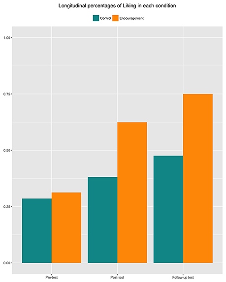
Figure 1. Percentages of vegetable liking in 37 preschool children, for the tree measurement moments (pre-test, post-test, and follow-up) and two reward systems (control vs. encouragement).

With model (1) defined, the research question of whether or not a reward system will increase the liking of chicory will amount to testing the null hypothesis H₀:β₁ = 0. When this null hypothesis is rejected, we will conclude that the reward system significantly increases (when β > 0) the probability of liking the vegetable. But how do we estimate and test the fixed effects and random intercept variance? Since there are myriad options and recommendations in current literature, and some of these may not yield satisfactory results for binary outcomes in such small clusters, we will introduce and compare several possibilities. As mentioned in the introduction, these estimation methods stem from both the GLMM- and SEM-frameworks; to this end, the next section provides an introduction of both frameworks, a short note on their equivalence, and an explanation of the difficulties that accompany marginalizing the GLMM-likelihood function over the random effects distribution.

3. Methods

3.1. Generalized Linear Mixed Models

Generalized linear mixed models (GLMMs) are basically extensions of Generalized Linear Models (GLMs) [29], which allow for correlated observations through the inclusion of random effects. Such effects can be interpreted as unobserved heterogeneity at the upper level, consequently inducing dependence among lower-level units from the same cluster.

Let x_ij and y_ij denote the ith measurement from cluster j, for the predictor and the binary outcome respectively (where i = 1, .., I and j = 1, …, J). Note that since we primarily focus on clusters of size two, we will set I to 2. Moreover, as I = 2 limits the identification of random effects, we will consider GLMMs with a random intercept only. In a fully parametric framework, this particular GLMM is typically formulated as:

$\begin{array}{cc}E(Y_{ij}|x_{ij},b_j)=g^{-1}({\beta }_0+{\beta }_1{x}_{ij}+b_j)\text{ with}{b}_j~N(0,\tau )& \left(2\right)\end{array}$

where g⁻¹(·) represents a known inverse link function, β₀ represents the intercept, β₁ the effect of the predictor x_ij, and b_j the cluster-specific random intercept. In this paper, we only consider probit regression models, where the standard normal cumulative distribution Φ(·) is defined as the inverse link function g⁻¹(·) [or equivalently the link function g(·) is defined as probit(·)]. Our reasoning behind this is that probit-regression applies to all estimation procedures we investigate, in contrast to the logit link. Converting Equation (2) to a random intercept probit-regression model yields us:

$\begin{array}{cc}P(y_{ij}=1\mid x_{ij},b_j)=\Phi ({\beta }_0+{\beta }_1{x}_{ij}+b_j)& \left(3\right)\end{array}$

In order to obtain estimates for β₀, β₁ and τ, the marginal likelihood function is typically maximized. For a random-intercept GLMM, this function is obtained by integrating out the cluster-specific random effect, and can be written as:

$\begin{array}{cc}l(\beta ,\tau |y_{ij})={\displaystyle \prod _{j=1}^J{\displaystyle {\int }_{-\infty }^{+\infty }{\displaystyle \prod _{i=1}^{I}f(y_{ij}|\beta ,b_j)\varphi (b_j|\tau )d{b}_j}}}& \left(4\right)\end{array}$

where f denotes the density function of the outcomes and ϕ the density of the random intercept (which is assumed to be normal here).

Unfortunately, statistical inference based on maximizing Equation (4) is hampered, because integrating out the random effects from the joint density of responses and random effects is, except for a few cases, analytically intractable. To tackle this, several techniques have been proposed, which can be divided into two main classes: likelihood-based methods and Bayesian approaches.

3.1.1. Estimation Through Likelihood-Based Approximation Methods

One way to tackle the intractability of integrating out the random effects of the GLMM likelihood function, is to either approximate the integrand or to approximate the integral itself. We briefly introduce three such methods below, and refer the interested reader to Tuerlinckx et al. [30] for more details.

Technically speaking, the Laplace approximation [31] approximates the integrand by a quadratic Taylor expansion. This results in a closed-form expression of the marginal likelihood, which can be maximized to obtain the maximum likelihood estimates of the fixed effects and random effect variances. In R, the implementation based on this approximation is available within the function glmer, from the package lme4 [32].

The Penalized Quasi-Likelihood method (PQL) [11, 33, 34] also approximates the integrand; more intuitively put, PQL approximates the GLMM with a linear mixed model. This is achieved by considering a Taylor expansion of the response function and by subsequently rewriting this expression in terms of an adjusted dependent variable on which estimation procedures for LMM can be implemented. Consequently, the algorithm cycles between parameter estimation by linear mixed modeling, and updating the adjusted dependent variable until convergence. This approach can be implemented using the function glmmPQL from the R-package MASS [35].

Finally, a tractable marginal likelihood can also be obtained by approximating the integral itself with a finite sum. In regular Gauss-Hermite (GH) Quadrature (e.g., [36]), this summation occurs over a fixed set of nodes, while Adaptive Gaussian Quadrature (AGQ) [37] uses a different set of nodes for each cluster. As such, when applying AGQ, fewer nodes are necessary to achieve equal accuracy as compared to the regular GH quadrature. AGQ estimation in R is also possible within the glmer function from lme4.

The detailed R-code on how to implement these three likelihood-based methods for a binary multilevel probit-model, can be found in the Supplementary Material (see Appendix - Likelihood-based methods). To check the R-implementation of AGQ against other software, we use the NLMIXED procedure within SAS^® [26].

3.1.2. Estimation Through Bayesian Methods

A second strategy that tackles the intractability of the GLMM likelihood function, pursues a Bayesian approach where Markov Chain Monte Carlo (MCMC) methods are used to obtain a posterior distribution of the parameters. MCMC methods simulate the likelihood rather than computing it, by calculating the sample average of independently simulated realizations of the integrand. As such, MCMC is thought to provide a more robust approach to marginalizing the random effects [18, 38].

In R, the MCMCglmm function from the package MCMCglmm [39] is available for such an approach. Technically, latent variables are updated in block by means of the Metropolis-Hastings algorithm [40–42], while the fixed parameters are Gibbs sampled within such a single block [43].

MCMC methods are known to be computationally intensive and sometimes have a hard time in reaching convergence. To this end, hybrid models based on an Integrated Nested Laplace Approximation (INLA) of the posterior marginals for latent Gaussian models [44] were proposed. In short, the INLA approach provides fast Bayesian inference by using accurate Laplace approximations for the marginal posterior density of the hyperparameter τ, and for the full conditional posterior marginal densities of the fixed and random effects. The final posterior marginals of the model parameters can then be computed through numerical integration, where the integration points are defaultly obtained by estimating the curvature of the approximation for the marginal posterior of the hyperparameter density [44]. Not surprisingly, these hybrids have shown a steep decline in the computational burden of MCMC algorithms, while at the same time converging more easily. In R, such an approach is implemented in the function inla from the package R-inla.

The detailed R-code of both implementations, as well as their prior specifications, can be found in the Supplementary Material (see Appendix - Bayesian methods). To check the R-based MCMC-implementation against other software, we rely on the he JAGS program [28] through the use of the R-package rjags [45]. It has been suggested by Betancourt and Girolami [46] that a non-centered parameterization of the hierarchal model works best when data are sparse, while a centered parameterization prevails when the data strongly identifies the parameters. However, we observed quite similar results stemming from the two parameterizations in our settings (results not shown).

3.2. Structural Equation Models

Although at first sight GLMM and SEM may seem like two completely different modeling frameworks, it is now well established that SEM can also be relied on to model balanced multilevel data structures. For an excellent overview of SEM, we refer the interested reader to Skrondal and Rabe-Hesketh [47]. In order to account for clustered observations, SEM lets its latent factors represent the random effects from their respective multilevel models [48, 49]. This results in a “conventional” SEM which is analytically equivalent to the corresponding multilevel model, under a broad set of conditions [4]; we illustrate this for model (2).

SEM consists of two modeling parts: a measurement model and a structural part [47]. The former defines unobserved variables in terms of observed variables measured with error, so that the latent variables can be interpreted as the “true” underlying variables (which might be correlated). The structural model on the other hand, links the different latent variables together. When focusing on random intercept models (read: with only one latent variable) with an explanatory variable in clusters of size two, both modeling-parts can be written as:

$\begin{array}{cc}\begin{array}{l}{y}_j=\nu +\Lambda {\eta }_j+K{x}_j+{ϵ}_j\\ {\eta }_j={\zeta }_j\end{array}& \left(5\right)\end{array}$

where y_j represents the responses within cluster j, ν = (ν ν) the vector of intercepts, η_j a latent variable with its matrix of factor loadings Λ = (1 1)^T, x_j = (x_1j x_2j)^T represents the explanatory variable, with K its matrix of regression coefficients, and ϵ_j = (ϵ_1j ϵ_2j)^T the vector of normally distributed measurement errors. In the structural part of the model, ζ_j represents a random disturbance term ~ N(0, τ). Note that in accordance to Equation (2), we assume the effect of x to be fixed within- as well as between clusters. Because of this, K reduces to $\left(\begin{array}{cc}k& 0\\ 0& k\end{array}\right)$. Alternatively, we can write the above equations in reduced form, resulting in:

$\begin{array}{cc}\begin{array}{l}{y}_j=\nu +K{x}_j+\Lambda {\zeta }_j+{ϵ}_j\\ =\nu +K{x}_j+{\zeta }_j+{ϵ}_j\end{array}& \left(6\right)\end{array}$

where ζ_j = (ζ_j ζ_j)^T.

Traditionally, estimation methods in SEM are based on the assumption that the observed responses are measured on a continuous scale. In order to reconcile SEM with binary outcomes, the Latent Response Variable approach was introduced, where a dichotomous Y is considered a crude approximation of an underlying continuous variable Y*. Y* is not directly observed (hence a latent response variable), and is written in terms of a linear predictor. When we separate the two observations within each cluster to eliminate matrix notations, we obtain:

$\begin{array}{cc}\{\begin{array}{ll}{y}_{1j}^{*}\hfill & =\nu +k{x}_{1j}+{\zeta }_j+{ϵ}_{1j}\hfill \\ y_{2j}^{*}\hfill & =\nu +k{x}_{2j}+{\zeta }_j+{ϵ}_{2j}\hfill \end{array}& \left(7\right)\end{array}$

where ϵ_1j and ϵ_2j are i.d.d. residuals of the latent response variables ~ N(0, θ). Because Y* exhibits an arbitrary mean and variance, a link between Y and Y* needs to be established through variance constraints. Since the variance of Y* conditional on x_ij is τ + θ, there are two possible ways to constrain this variance [50]. First, Generalized Linear Models standardly fix the residual variance θ to one. In contrast to this theta parameterization, identification can also be achieved by standardizing the latent variable Y* itself: the delta parameterization fixes the the sum of τ and θ to one. This parameterization is traditionally used in the SEM-literature.

The relationship between the binary and latent continuous variable is then: Y = 1⇔Y* > κ. Fixing the threshold κ at 0 (for model identifiability, either the threshold or the intercept in Equation (7) needs to be constrained), and assuming that $Y_{ij}^{*}~N(0,1)$ (i.e., making use of the delta parametrization so that ζ_j ~ N(0, τ_δ) and ϵ_ij ~ N(0, 1 − τ_δ)), it follows that:

$\begin{array}{cc}\begin{array}{l}E[Y_{ij}|x_{ij},{\zeta }_j]=P(\nu +k{x}_{ij}+{\zeta }_j+{ϵ}_{ij}>0|x_{ij},{\zeta }_j)\\ =P({ϵ}_{ij}<\nu +k{x}_{ij}+{\zeta }_j|x_{ij},{\zeta }_j)\\ =P(\frac{{ϵ}_{ij}}{\sqrt{1-{\tau }_{\delta }}}<\frac{\nu +k{x}_{ij}+{\zeta }_j}{\sqrt{1-{\tau }_{\delta }}}|x_{ij},{\zeta }_j)\\ =\Phi (\frac{\nu }{\sqrt{1-{\tau }_{\delta }}}+\frac{k{x}_{ij}}{\sqrt{1-{\tau }_{\delta }}}+\frac{{\zeta }_j}{\sqrt{1-{\tau }_{\delta }}})\end{array}& \left(8\right)\end{array}$

which reduces to the random intercept probit-model from Equation (3), where $\frac{\nu }{\sqrt{1-{\tau }_{\delta }}}$, $\frac{k}{\sqrt{1-{\tau }_{\delta }}}$ and $\frac{{\zeta }_j}{\sqrt{1-{\tau }_{\delta }}}$ are equivalent to β₀, β₁, and b_j, respectively.

3.2.1. Estimation in SEM

Within the SEM-framework, there are two common estimation approaches for modeling binary outcomes: maximum likelihood (ML) estimation and weighted least squares (WLS) [47]. In contrast to WLS, ML estimation for binary outcomes is not widely available in SEM software. Being a “full information” method, ML is more regularly employed in item response theory [51]. In contrast, as WLS-based methods adopt a multiple-step estimation procedure in which only first- and second-order information from the data is used, they are referred to as a “limited information” approach (see [52] for a review). In SEM, WLS is employed to differentially weigh the residuals resulting from the observed vs. the model-implied sample statistics by their full asymptotic covariance matrix W.

Since WLS requires extremely large samples for accurate estimation of the weight matrix W, more contemporary approaches were developed to improve small sample performance. One such version entails diagonally weighted least squares (DWLS), which utilizes a diagonal weight matrix instead of a full one [53, 54] (note that statistical inference in DWLS still relies on the full weight matrix, even when a diagonal matrix is used during estimation). Following Muthén et al. [54], who have shown DWLS to be statistically and computationally efficient in large samples, more recent studies have proven that DWLS is also more stable than WLS in small samples [51, 55, 56]. Note that WLS and DWLS estimation is limited to probit-regression models and therefore exclude logit-models from our current review study.

SEM relying on DWLS can be implemented through the sem- function from the package lavaan [57]. The detailed R-code of this implementation can be found in the Supplementary Material (see Appendix - SEM methods). To check the lavaan package against other implementations, we will verify our results with DWLS estimation in MPLUS^® software [27] through the use of the R-package MplusAutomation [58].

4. Analysis of the Example

We illustrate the above six approaches by applying them to our example. To assess the impact of cluster size, we consider the fit of model (1) when solely looking at the pre- and post-test (i.e., cluster size two) vs. all three time points together (i.e., cluster size three). The estimated parameters for the fixed effects (and their standard errors), alongside the estimated random intercept variance for each of the estimation approaches are summarized in Table 1.

TABLE 1

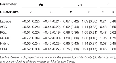
Table 1. The estimates (and (robust) standard errors) from the six approaches for the intercept β₀, the slope parameter β₁ and the random intercept variance τ.

We observe that for both cluster sizes all methods perform rather similar in their estimation of β₀, except for a higher estimate produced by MCMC. The estimates for β₁ show more variation, especially within clusters of size two (again with an outlying MCMC-estimate). For the random intercept variance τ, we see that the MCMC estimate is somewhat larger than the others, while the estimates from the Laplace approximation and the hybrid approach are at the lower end of this spectrum. In terms of computing times, most approaches performed equivalently, with the Laplace approximation providing the fastest analysis, closely followed by AGQ, SEM and PQL. The MCMC approach took about ten times as long as the aforementioned approaches, while the hybrid approach only increased the computing time threefold.

Now the question becomes: which of these estimation methods is most reliable here? In order to find out, we conduct an extensive simulation study in the next section.

5. Simulation Study

In our simulation study we compare the performance of the six above-described estimation methods in different settings. For this, random binary outcome variables from small clusters are generated under a random intercept probit-regression model (see Supplemantary Material - Data Generating Mechanism). More specifically, we assume an underlying latent variable $Y_{ij}^{*}$, such that Y_ij = 1 if $Y_{ij}^{*}>0$:

$\begin{array}{cc}P(Y_{ij}=1|x_{ij},b_j)=P(Y_{ij}^{\ast }>0|x_{ij},b_j)& \left(9\right)\end{array}$

$\begin{array}{cc}\begin{array}{l}=P({\beta }_0+{\beta }_1{x}_{ij}+b_j+{ϵ}_{ij}>0),\\ b_j~N(0,\tau )\text{and}{ϵ}_{ij}~N(0,1)\end{array}& \left(10\right)\end{array}$

First of all, we consider different cluster sizes: we will look at clusters of size two, three and five. Second, we also consider a different numbers of clusters. Since, Loeys et al. [59] reported that sample sizes in studies using the Actor-Partner- Interdependence-Model [60] within dyads typically ranged from 30 to 300 pairs, we consider sample sizes n of 25, 50, 100, and 300. Third, we also examine different intracluster correlations (icc) for the latent response variable. As the latent icc_l is defined as the proportion of between-group vs. total variance in Y* ($ic{c}_l=\frac{Var(b_j)}{Var(Y_{ij}^{*})}=\frac{\tau }{\tau +1}$), a latent icc_l of 0.10, 0.30, and 0.50 corresponds to a random intercept variance of 0.11, 0.43, and 1.00, respectively. Fourth, we consider rare as well as more abundant outcomes, with an overall event rate of 10 and 50%, respectively. Since the marginal expected value of the outcome E(Y) equals $\Phi (\frac{{\beta }_0}{\sqrt{1.25+\tau }})$, an outcome prevalence of 50% implies that β₀ must be set to zero. Equivalently, when fixing β₀ to −1.50, −1.66, and −1.92 for a random intercept variance τ = 0.11, 0.43, and 1, respectively, an outcome prevalence of 10% is obtained². In all simulations, β₁ is fixed to 1. Finally, four types of covariates are compared: we consider a predictor that only varies between clusters, vs. one that varies within clusters; and a Gaussian distributed predictor ~ N(0, 0.25), vs. a zero-centered Bernoulli x with success rate 0.5.

In total, 2000 simulations are generated for the 3 × 4 × 3 × 2 × 4 combinations of clusters size (3), sample size (4), intracluster correlation (3), outcome prevalence (2) and type of predictor (4). The above-introduced methods are compared over these 288 settings in terms of convergence, relative bias, mean squared error (MSE) and coverage. The relative bias is defined as the averaged difference between the estimated (e.g., $\widehat{\beta }$) and true parameter values (e.g., β), divided by the latter (so that the relative bias $=\frac{\beta -\widehat{\beta }}{\beta }$); as such, a relative bias enclosing zero will indicate an accurate estimator. A relative bias measure was chosen over an absolute one, as the accuracy of some procedures tends to depend on the magnitude of the parameter values [63]. The MSE is estimated by summing the empirical variance and the squared bias of the estimates, simultaneously assessing bias and efficiency: the lower the MSE, the more accurate and precise the estimator. The coverage is defined as the proportion of the 95%-confidence intervals that encompass their true parameter value, where coverage rates nearing 95% represent nominal coverages of the intervals. For the likelihood-based and SEM approaches, Wald confidence intervals are used, while the Bayesian approaches rely on the quantile-based 95% posterior credible intervals. Note that coverage rates for τ are not provided, as not all estimation procedures provide this interval. Lastly, in order to conclude model convergence, several criteria must be met: first, whenever fixed effect estimates exceed an absolute value of ten, or the random effect estimate exceeds 25, the fit is classified as “no convergence.” We decided on this as parameters in a probit-regression exceeding an absolute value of five are extremely unlikely for the given covariate distribution and effect sizes. Secondly, convergence has also failed when a model fit does not yield estimators or standard errors. In addition, for MCMCglmm we specified that both chains must reach convergence as assessed by Geweke diagnostics; only when this statistic is smaller than two, convergence is concluded. To ensure a fair comparison between methods, we only present results for simulation runs in which all six methods converged.

6. Results

Below, we discuss the results of the simulation study for clusters of size two with a Gaussian predictor in detail.

6.1. Convergence

Generally, convergence improves as the number of clusters and the outcome prevalence increase, and as the icc_l decreases (see Figure 2). In contrast, convergence is rather unaffected by the level of the predictor, except for PQL which tends to show more convergence difficulties for a within-cluster x. The Laplace approximation also shows a slight decline in convergence for rare outcomes combined with a within-cluster predictor. Note that for 300 clusters most approaches reach 100% convergence, except for MCMC (as in Ten Have and Localio [21]) and at times the Laplace approximation. For rare outcomes in small samples (n = 25), however, the hybrid approach and SEM (see e.g., [51, 64]) often perform worse than MCMC. Overall, AGQ shows least difficulty in reaching convergence.

FIGURE 2

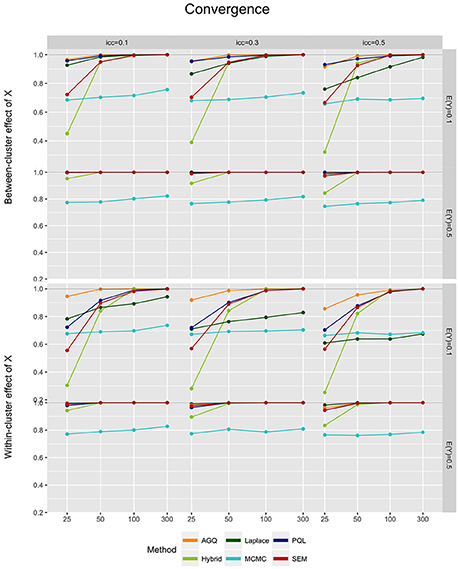
Figure 2. Model convergence of the six approaches, for different measurement levels of X (within- or between clusters), outcome prevalence (0.1 and 0.5), icc_l (0.1, 0.3, and 0.5), and sample size (25, 50, 100, and 300).

6.2. Relative Bias

First, for the fixed effect estimators we typically observe that the relative bias decreases as the number of clusters increases (see Figure 3). The Laplace approximation and PQL contradict this, however: for rare outcomes the relative bias tends to increase with n. Second, we see that an increase in the icc_l tends to shift the relative bias downwards. This implies an improvement in the performance of MCMC (in contrast to Ten Have and Localio [21]), but not of most other methods [65–68]. As such, we observe that MCMC performs worse than most methods, but that this difference attenuates as the icc_l increases. Third, the relative bias is generally smaller for a 0.5 outcome prevalence, compared to rare events; this is most clear for the hybrid approach, but is also visible in AQG (see [69]). For an outcome prevalence of 0.5, the bias in the β₀-estimators even becomes negligible for all methods. For β₁, however, the MCMC method actually performs worse in small samples when E(Y) = 0.5, compared to 0.1. Fourth, different measurement levels of the predictor do not much sway the bias, except for PQL; this method reveals slightly more bias for low event rates when the predictor is measured within- rather than between-clusters. Overall, SEM provides the least biased estimators for the fixed effects, closely followed by AGQ.

FIGURE 3

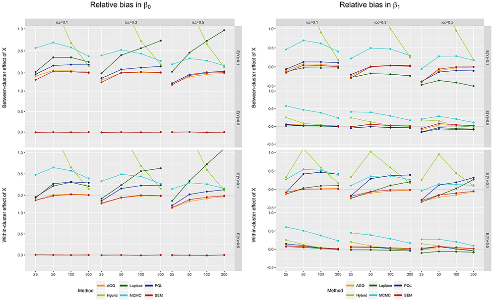
Figure 3. Relative bias in β₀ (left) and β₁ (right) for the six approaches, for different measurement levels of X (within- or between clusters), outcome prevalence (0.1 and 0.5), icc_l (0.1, 0.3, and 0.5), and sample size (25, 50, 100, and 300). These results stem from simulation runs where all methods converged.

For the variance of the random effect, better estimators are typically found in larger samples (see left part of Figure 4, also see Hox [68]). Similar to the fixed effect estimators, the Laplace approximation and PQL pose an exception to this rule, by inverting this relation for rare outcomes (see [70]). As such, the conclusions of Capanu et al. [20], stating that the hybrid approach outperforms the Laplace approximation by reducing bias in τ, do hold here, but only for large n. We also observe that as the icc_l decreases, bias in the estimates for τ increases in all methods. Finally, a slightly negative bias in the AGQ- and SEM-estimates for τ is observed when the outcome is rare and n small [2]. This negative bias, however, attenuates as the number of clusters is increased [70]. Overall, SEM yields the least biased estimators for the random intercept variance when the outcome prevalence is rare, while AGQ performs best when E(Y) = 0.5.

FIGURE 4

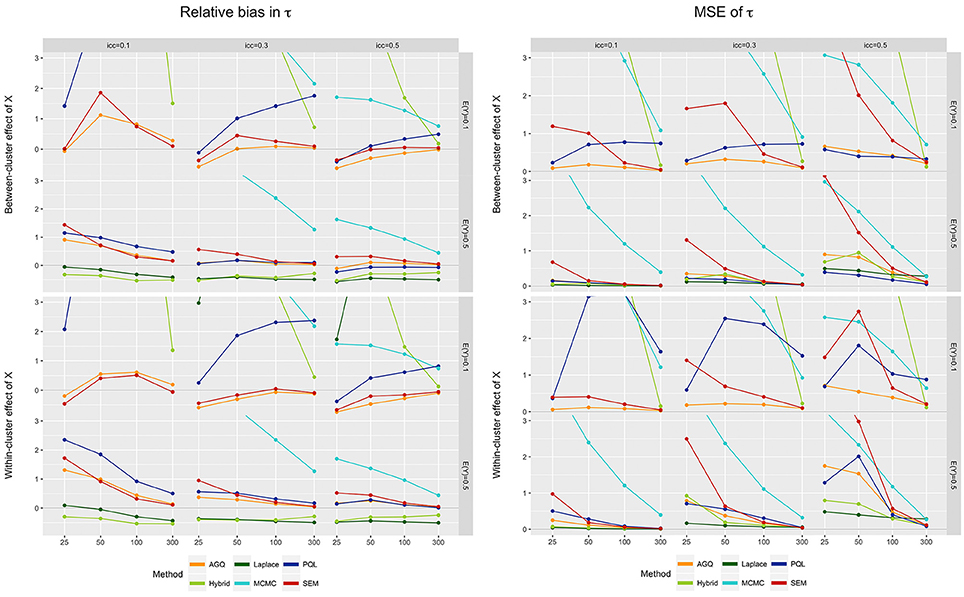
Figure 4. Relative bias (left) and MSE (right) of τ for the six approaches, for different measurement levels of X (within- or between clusters), outcome prevalences (0.1 and 0.5), icc_l (0.1, 0.3, and 0.5), and sample sizes (25, 50, 100, and 300). These results stem from simulation runs where all methods converged.

6.3. MSE

For both β₀ and β₁, the MSE is often higher for rare outcomes, compared to a 0.5 prevalence (see Figure 5). Additionally, the MSE drops as the sample size grows, and as the icc_l decreases. The Laplace estimator for β₀ again contradicts these trends: for rare events, the MSE increases with sample size and icc_l. As before, the measurement level of x does not much alter performance, except in PQL where a within-cluster predictor slightly increases the MSE. For both fixed effects, MCMC often yields the highest MSE when the prevalence equals 0.5, while the hybrid approach regularly performs worst for a prevalence of 0.1. In general, the Laplace approximation yields the lowest MSE when E(Y) = 0.5, but performs much worse when the outcome is rare. Overall, AGQ (closely followed by SEM) performs best in terms of MSE.

FIGURE 5

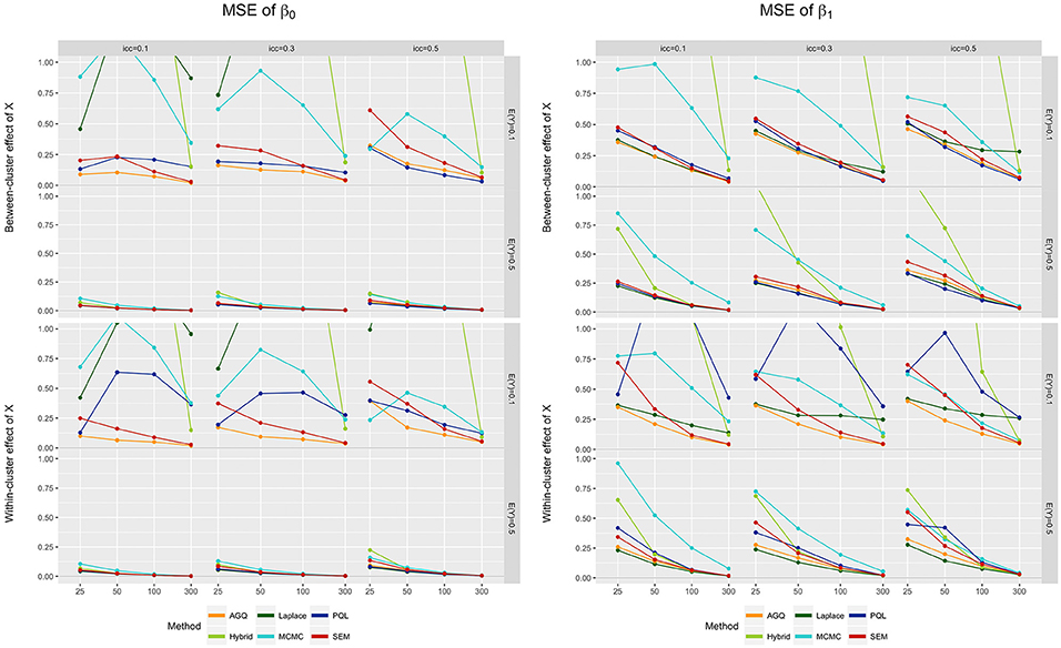
Figure 5. MSE of β₀ (left) and β₁ (right) for the six approaches, for different measurement levels of X (within- or between clusters), outcome prevalences (0.1 and 0.5), different icc_l (0.1, 0.3, and 0.5), and sample sizes (25, 50, 100, and 300). These results stem from simulation runs where all methods converged.

For the random intercept variance τ, we observe a decrease in MSE as the sample size increases, and as the icc_l decreases (see right part of Figure 4). The latter conclusion does not hold for MCMC as here the MSE tends to decrease with rising icc_l. Again, PQL performs slightly worse for a within-cluster predictor. In general, the Laplace approximation yields the lowest MSE for 0.5 prevalences, but performs worst when the outcome is rare. Overall, AGQ performs best in terms of MSE, better than SEM, especially in smaller samples.

6.4. Coverage

For both fixed effect estimators, coverage of their 95% confidence intervals is typically better when the outcome prevalence is 0.5 (see Figure 6). Also, an increasing icc_l usually worsens coverage, except for MCMC (where coverage improves with increasing icc [21]). The impact of the icc_l on coverage has also been observed by Zhang et al. [63], who found nominal coverages for AGQ and the Laplace approximation for low random intercept variances (i.e., low icc), but more liberal ones as τ increases (i.e., high icc). Generally, SEM and AGQ provide the best coverage rates [70], with SEM taking the upper hand for the coverage of β₀, and AGQ for β₁ with a low to medium icc.

FIGURE 6

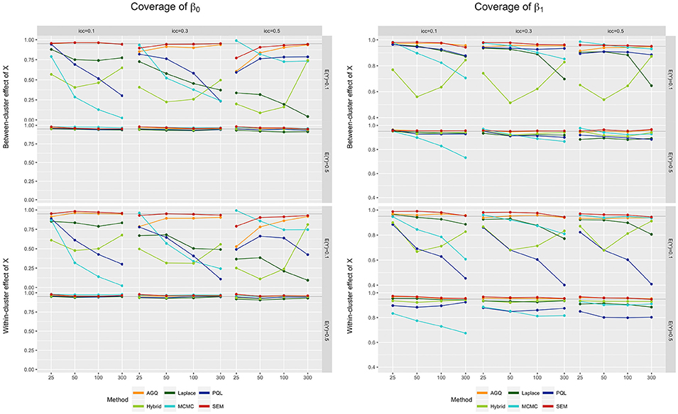
Figure 6. Coverage of β0 (left) and β₁ (right) for the six approaches, for different measurement levels of X (within- or between clusters), outcome prevalences (0.1 and 0.5), icc_l (0.1, 0.3, and 0.5), and sample sizes (25, 50, 100, and 300). These results stem from simulation runs where all methods converged.

6.5. Summary of the Other Simulation Settings

Until now, we only discussed the results of the simulation study for clusters of size two with a Gaussian predictor. The results for other settings are available in the Supplementary Material and are briefly discussed in the next paragraphs.

When looking at a binary predictor instead of a Gaussian one, our conclusions remain more or less the same. One exception is that most methods experience a steep decline in convergence for smaller sample sizes, when the predictor is binary compared to continous. This is most apparent in SEM, where lower convergence rates are due to empty cell combinations of outcome and predictor. In SEM, this produces a warning, which we interpreted as an error (as in MPLUS), since such runs yield unreliable results.

As the cluster size increases from two to three or five, we observe a general increase in performance in all methods except SEM. This approach now no longer yields the lowest bias, with AGQ gradually taking over. As such, increasing cluster size favors AGQ in terms of precision, as well as in terms of relative bias.

6.6. MPLUS, JAGS, and SAS

MPLUS and lavaan performed quite similarly throughout our settings, although there were some minor differences (results shown in the Supplementary Material). While MPLUS version 7 slightly dominates in terms of convergence and coverage, lavaan takes the upper hand for the relative bias and the MSE. These differences are trivial, however, and most likely due to lavaan incorporating a slightly higher number of iterations in reaching convergence.

When comparing JAGS to MCMCglmm, we observe some important differences in performance; for most settings, JAGS 4.1.0. outperforms MCMCglmm, except when a small n is combined with a medium to large icc_l (see Supplementary Material). Note that although JAGS performs slightly better in most settings, its computing times are also significantly higher.

In contrast to Zhang et al. [63], who found a superior performance of SAS NLMIXED compared to R's glmer-function, we found that glmer performed equally well or even slightly better in terms of convergence rates, relative bias, and coverage (using SAS version 9.4). When the outcome prevalence is 0.5 and for some rare events settings, glmer also provided a slightly lower MSE.

7. Discussion

In this paper, we provided an overview of several R-packages based on different estimation techniques, as to fit random-intercept probit regression models. More specifically, we focused on techniques capable of modeling binary outcomes in small clusters. Additionally, we presented an extensive simulation study in which we assessed the impact of various data features on a number of performance criteria. In summary, we found that some of our results confirmed findings from previous studies, while others have (to the best of our knowledge) not been observed before:

Interestingly, both SEM and AGQ performed considerably well for paired data. Though both approaches disclosed some sensitivity to sample size, they manifested remarkable robustness when varying the icc, the event rate, and the measurement level of the predictor. As such, these methods can be considered the most stable over all settings in terms of relative bias, for the fixed effect regression coefficients as well as the random intercept variance. While AGQ performs slightly better than SEM in terms of convergence and MSE, SEM performs slightly better when considering the relative bias. As SEM relies on robust standard errors, it yields higher MSE's, but also provides robustness against model misspecification (which was not investigated here). For the coverage, we observed that SEM performs slightly better for β0, while AGQ tentatively gains the upper hand for β₁. As the cluster size increases, however, AGQ takes over and becomes most reliable in terms of bias and precision.

Since the Laplace approximation is known to be precise only for normally distributed data or for non-normal data in large clusters [30], we observed an expected poor performance of this approximation in our settings [23]. PQL also exhibits an inferior performance for low icc's and a low outcome prevalence, while additionally revealing disconcerting performance issues for a within-cluster measured predictor. Finally, the two Bayesian approaches performed below par in terms of most criteria considered.

Let us once again consider our motivating example with a within-cluster measured predictor, a sample size of 37, an outcome prevalence of 0.4, and a medium to large latent icc. When we apply our conclusions to these settings, we can state that SEM will yield the most trustworthy estimates when the cluster size is two, while AGQ will take over as a measurement is added. MCMC will yield the most biased estimates in both cases (as can be clearly seen in Table 1).

Several limitations can still be ascribed to this paper. First, we restricted our comparisons to estimation techniques available in R-packages. As such, several improvements regarding the estimation methods discussed, could not be explored. For example, while the glmmPQL function employed in this paper is based on Breslow and Clayton [11]'s PQL version, a second-order Taylor expansion [71] might provide a more precise linear approximation (this is referred to as PQL-2, in contrast to the first order version PQL-1). Be that as it may, not all the evidence speaks in favor of PQL-2: even though it yields less bias than PQL-1 when analyzing binary outcomes, Rodriguez [72] found that the estimates for both fixed and random effects were still attenuated for PQL-2. Furthermore, PQL-2 was found to be less efficient and somewhat less likely to converge [72]. Second, certain choices were made with respect to several estimation techniques, such as the number of quadrature points used in the AGQ-procedure. However, acting upon the recommendation of 8 nodes for each random effect [17], we argue that surpassing the ten quadrature points considered, would carry but little impact in our random intercept model. Also, the repercussions of our choices on prior specification in the Bayesian framework deserves a more thorough examination, as different priors may lead to somewhat different findings. Third, the performance results presented here may not be intrinsic to their respective estimation techniques, but instead due to decisions made during implementation. As we demonstrated for MCMCglmm when comparing it to JAGS, its disappointing performance is most likely due to a suboptimal implementation, and not an inherent treat of the MCMC estimation procedure. Fourth, some scholars [73] have recommended the evaluation of different estimation methods and their dependence on different data features, by applying ANOVA-models rather than graphical summaries. Treating the different settings (sample size, icc, level of the predictor, the event rate, and their two-way interactions) as factors, did not provide us much insight since almost all variables (as well as their interactions) were found to be highly significant. Fifth, in our simulation study we only considered complete data; in the presence of missing data, however, DWLS estimation in SEM will exclude clusters with one or more missing outcomes, resulting in a complete case analysis. This exclusion stands in contrast to maximum likelihood and Bayesian approaches from the GLMM-framework, as they consider all available outcomes when there is missingness present. Consequently, the GLMM-framework will not introduce any (additional) bias under the missing at random assumption, while DWLS-estimation requires the more stringent assumption of data missing completely at random. Sixth, we do not focus on measurement imprecision in this study and assume that all observed variables are measured without error. Of course, as Westfall and Yarkoni [74] recently pointed out, this rather optimistic view might pose inferential invalidity when this assumption fails. In light of this, it is important to note that SEM can deal with such measurement error, in contrast to GLMM-based approaches.

With the results, as well as the limitations of the current paper in mind, some potential angles for future research might be worth considering. As we explicitly focused on conditional models, we deliberately excluded marginal approaches such as Generalized Estimating Equations (GEE), because such a comparison is impeded by the fact that marginal and conditional effects differ for binary outcomes. Whereas, multilevel models allow for the separation of variability at different levels by modeling the cluster-specific expectation in terms of the explanatory variables, GEE only focuses on the respective marginal expectations. Previous research [75] has revealed excellent small sample performance of GEE in terms of bias, when analyzing binary data in clusters of size two. Also, it might we worth considering a pairwise maximum likelihood (PML) approach, as PML estimators have the desired properties of being normally distributed, asymptotically unbiased and consistent [76]. This estimation method breaks up the likelihood into little pieces and consequently maximizes a composite likelihood of weighted events. PML in R is currently unable to cope with predictors, but this will most likely be possible in the near future. And finally, as pointed out by one of the reviewers, Hamiltonian Monte Carlo (used in Stan software, Carpenter et al. [77]) may be a more efficient sampler compared to a Metropolis-Hastings (i.e., MCMCglmm) or a Gibbs sampler (i.e., JAGS). To this end, exploring the performance of the Stan software might prove worthwhile when further focusing on Bayesian analysis.

Author Contributions

HJ performed the analysis of the example, conducted the simulation studies, and wrote the paper. TL participated in the writing and reviewing of the paper, alongside checking the analyses and simulations. YR critically reviewed and proof-read the entire manuscript.

Conflict of Interest Statement

The authors declare that the research was conducted in the absence of any commercial or financial relationships that could be construed as a potential conflict of interest.

Acknowledgments

This work was carried out using the Stevin Supercomputer Infrastructure at Ghent University provided by the VSC (Flemish Supercomputer Centre), funded by Ghent University, the Hercules Foundation and the Flemish Government - department EWI.

Supplementary Material

The Supplementary Material for this article can be found online at: https://www.frontiersin.org/article/10.3389/fams.2016.00018

Footnotes

1. ^SAS and all other SAS Institute Inc. product or service names are registered trademarks or trademarks of SAS Institute Inc. in the USA and other countries. ^® indicates USA registration.

2. ^Note that the observed icc_o is dependent on the intercept β₀, the random intercept variance τ, and the latent icc_l through the following formula [61]: $ic{c}_o=\frac{{\Phi }_2(\frac{{\beta }_0}{\sqrt{(\tau +1)(1+2\tau )}},\frac{{\beta }_0}{\sqrt{\tau +1}},ic{c}_l)-{\Phi }_1{(\frac{{\beta }_0}{\sqrt{\tau +1}})}^2}{{\Phi }_1(\frac{{\beta }_0}{\sqrt{\tau +1}})(1-{\Phi }_1(\frac{{\beta }_0}{\sqrt{\tau +1}}))}$. In this equation, Φ₁ represents the cumulative standard normal distribution, and Φ₂ the cumulative bivariate standard normal distribution with correlation icc_l. Since the outcome prevalence dictates the value of the intercept, each combination of icc_l and E(Y) provides different icc_o's; for rare outcomes, the observed icc_o are 0.06, 0.25, and 0.51, while for E(Y) = 0.5 they are 0.06, 0.19, and 0.33 (corresponding to latent icc_l's of 0.10, 0.30, and 0.50, respectively). As such, the observed icc_o's range from small to large, according to Hox [62]'s recommendations.

References

1. Snijders T, Bosker R. Multilevel Analysis: An Introduction to Basic and Advanced Multilevel Modeling. Thousand Oaks, CA: Sage (1999).

2. Raudenbush S, Bryk A. Hierarchal Linear Models. Applications and Data Analysis Methods. 2nd Edn., Thousand Oaks, CA: Sage (2002).

3. Rovine MJ, Molenaar PC. A structural modeling approach to a multilevel random coefficients model. Multiv Behav Res. (2000) 35:55–88. doi: 10.1207/S15327906MBR3501_3

PubMed Abstract | CrossRef Full Text | Google Scholar

4. Curran PJ. Have multilevel models been structural equation models all along? Multiv Behav Res. (2003) 38:529–69. doi: 10.1207/s15327906mbr3804_5

PubMed Abstract | CrossRef Full Text | Google Scholar

5. Bauer DJ. Estimating multilevel linear models as structural equation models. J Educ Behav Stat. (2003) 28:135–67. doi: 10.3102/10769986028002135

CrossRef Full Text | Google Scholar

6. Airy G. On the Algebraical and Numerical Theory of Errors of Observations and the Combination of Observations. London: Macmillan (1861).

Google Scholar

7. Scheffé H. The analysis of variance. New York, NY: John Wiley & Sons (1959).

8. Harville DA. Maximum likelihood approaches to variance component estimation and to related problems. J Am Stat Assoc. (1977) 72:320–38. doi: 10.1080/01621459.1977.10480998

CrossRef Full Text | Google Scholar

9. Laird NM, Ware JH. Random-effects models for longitudinal data. Biometrics (1982) 38:963–74. doi: 10.2307/2529876

PubMed Abstract | CrossRef Full Text | Google Scholar

10. Goldstein H. The Design and Analysis of Longutudinal Studies. London: Academic Press (1979).

11. Breslow NE, Clayton DG. Approximate inference in generalized linear mixed models. J Am Stat Assoc. (1993) 88:9–25.

Google Scholar

12. Rodriguez G, Goldman N. An assessment of estimation procedures for multilevel models with binary responses. J R Stat Soc Ser A (1995) 158:73–89. doi: 10.2307/2983404

CrossRef Full Text | Google Scholar

13. McMahon JM, Tortu S, Torres L, Pouget ER, Hamid R. Recruitment of heterosexual couples in public health research: a study protocol. BMC Med Res Methodol. (2003) 3:24. doi: 10.1186/1471-2288-3-24

PubMed Abstract | CrossRef Full Text | Google Scholar

14. Glynn RJ, Rosner B. Regression methods when the eye is. Ophthalm Epidemiol. (2013) 19:159–65. doi: 10.3109/09286586.2012.674614

PubMed Abstract | CrossRef Full Text | Google Scholar

15. Ortqvist AK, Lundholm C, Carlström E, Lichtenstein P, Cnattingius S, Almqvist C. Familial factors do not confound the association between birth weight and childhood asthma. Pediatrics (2009) 124:e737–43. doi: 10.1542/peds.2009-0305

PubMed Abstract | CrossRef Full Text | Google Scholar

16. Senn S. Cross-Over Trials in Clinical Research. Chichester: John Wiley & Sons (2002). doi: 10.1002/0470854596

CrossRef Full Text | Google Scholar

17. Rabe-hesketh S, Pickles A. Reliable estimation of generalized linear mixed models using adaptive quadrature. Stata J. (2002) 2:1–21.

Google Scholar

18. Browne WJW, Draper D. A comparison of Bayesian and likelihood-based methods for fitting multilevel models. Bayes Anal. (2006) 1:473–514. doi: 10.1214/06-BA117

CrossRef Full Text | Google Scholar

19. Zhang Z, Zyphur MJ, Preacher KJ. Testing multilevel mediation using hierarchical linear models. Organ Res Methods (2009) 12:695–719. doi: 10.1177/1094428108327450

CrossRef Full Text | Google Scholar

20. Capanu M, Gönen M, Begg CB. An assessment of estimation methods for generalized linear mixed models with binary outcomes. Stat Med. (2013) 32:4550–66. doi: 10.1002/sim.5866

PubMed Abstract | CrossRef Full Text | Google Scholar

21. Ten Have TR, Localio AR. Empirical Bayes estimation of random effects parameters in mixed effects logistic regression models. Biometrics (1999) 55:1022–9. doi: 10.1111/j.0006-341X.1999.01022.x

PubMed Abstract | CrossRef Full Text | Google Scholar

22. Sutradhar BC, Mukerjee R. On likelihood inference in binary mixed model with an application to COPD data. Comput Stat Data Anal. (2005) 48:345–61. doi: 10.1016/j.csda.2004.02.001

CrossRef Full Text | Google Scholar

23. Broström G, Holmberg H. Generalized linear models with clustered data: fixed and random effects models. Comput Stat Data Anal. (2011) 55, 3123–34. doi: 10.1016/j.csda.2011.06.011

CrossRef Full Text | Google Scholar

24. Xu Y, Lee CF, Cheung YB. Analyzing binary outcome data with small clusters: A simulation study. Commun Stat Simul Comput. (2014) 43:1771–82. doi: 10.1080/03610918.2012.744044

CrossRef Full Text | Google Scholar

25. R Core Team. R: A Language and Environment for Statistical Computing. Vienna: R Foundation for Statistical Computing (2013).

Google Scholar

26. SAS Institute Inc. Base SAS® 9.4 Procedures Guide, Fifth Edition. Cary, NY: SAS Institute Inc. (2015).

27. Muthén LK, Muthén BO. Mplus User's Guide. 6th Edn., Los Angeles, CA: Muthén & Muthén (2010).

28. Plummer M. JAGS : A program for analysis of Bayesian graphical models using Gibbs sampling. In: Hornik K, Leisch F, Zeileis A, editors. Proceedings of the 3rd International Workshop on Distributed Statistical Computing (DSC 2003). Vienna, Austria (2003). p. 1–10.

29. Nelder J, Wedderburn R. Generalized linear models. J R Stat Soc Ser A (1972) 135:370–84. doi: 10.2307/2344614

CrossRef Full Text | Google Scholar

30. Tuerlinckx F, Rijmen F, Verbeke G, De Boeck P. Statistical inference in generalized linear mixed models: a review. Br J Math Stat Psychol. (2006) 59, 225–55. doi: 10.1348/000711005X79857

PubMed Abstract | CrossRef Full Text | Google Scholar

31. Tierney L, Kadane JB. Acccurate approximations for posterior moments and marginal densities. J Am Stat Assoc. (1986) 81:82–6. doi: 10.1080/01621459.1986.10478240

CrossRef Full Text | Google Scholar

32. Bates D, Maechler M, Bolker B, Walker S. Fitting linear mixed-effects models using lme4. J. Stat. Softw. (2015) 67:1–48. doi: 10.18637/jss.v067.i01

CrossRef Full Text

33. Schall R. Estimation in generalized linear models with random effects. Biometrika (1991) 78:719–27. doi: 10.1093/biomet/78.4.719

CrossRef Full Text | Google Scholar

34. Stiratelli R, Laird N, Ware J. Random-effects models for serial observations with binary response. Biometrics (1984) 40:961–71. doi: 10.2307/2531147

PubMed Abstract | CrossRef Full Text | Google Scholar

35. Venables WN, Ripley BD. Modern Applied Statistics with S. New York, NY: Springer (2002). doi: 10.1007/978-0-387-21706-2

CrossRef Full Text | Google Scholar

36. Naylor J, Smith A. Applications of a method for the efficients computation of posterior distributions. Appl Stat. (1982) 31:214–25. doi: 10.2307/2347995

CrossRef Full Text | Google Scholar

37. Pinheiro JC, Bates DM. Approximations to the log-likelihood function in the nonlinear mixed-effects model. J Comput Graph Stat. (1995) 4:12–35.

Google Scholar

38. Zhao Y, Staudenmayer J, Coull Ba, Wand MP. General design Bayesian generalized linear mixed models. Stat Sci. (2006) 21:35–51. doi: 10.1214/088342306000000015

CrossRef Full Text

39. Hadfield JD. MCMC methods for multi-respoinse generalized linear mixed models: The MCMCglmm R package. J Stat Softw. (2010) 33:1–22. doi: 10.18637/jss.v033.i02

CrossRef Full Text | Google Scholar

40. Metropolis N, Rosenbluth AW, Rosenbluth MN, Teller AH, Teller E. Equation of state calculations by fast computing machines. J Chem Phys. (1953) 21:1087–92. doi: 10.1063/1.1699114

CrossRef Full Text | Google Scholar

41. Hastings WK. Monte Carlo sampling methods using Markov chains and their applications. Biometrika (1970) 57:97–109. doi: 10.1093/biomet/57.1.97

CrossRef Full Text | Google Scholar

42. Tierney L. Markov chains for exploring posterior distributions. Ann Stat. (1994) 22:1701–28. doi: 10.1214/aos/1176325750

CrossRef Full Text | Google Scholar

43. García-Cortés LA, Sorensen D. Alternative implementations of Monte Carlo EM algorithms for likelihood inferences. Genet Select Evol. (2001) 33:443–52. doi: 10.1051/gse:2001106

PubMed Abstract | CrossRef Full Text | Google Scholar

44. Rue H, Martino S, Chopin N. Approximate Bayesian inference for latent Gaussian models by using integrated nested Laplace approximations. J R Stat Soc Ser B (2009) 71:319–92. doi: 10.1111/j.1467-9868.2008.00700.x

CrossRef Full Text | Google Scholar

45. Plummer M. rjags: Bayesian Graphical Models using MCMC (2016). Available online at: https://cran.r-project.org/package=rjags

46. Betancourt MJ, Girolami M. Hamiltonian monte carlo for hierarchical models. ArXiv e-prints (2013). doi: 10.1201/b18502-5

PubMed Abstract | CrossRef Full Text | Google Scholar

47. Skrondal A, Rabe-Hesketh S. Generalized Latent Variable Modeling: Multilevel, Longitudinal, and Structural Equation Models. Boca Raton, FL: Chapman & Hall/CRC (2004). doi: 10.1201/9780203489437

CrossRef Full Text | Google Scholar

48. Willett JB, Sayer AG. Using covariance structure analysis to detect correlates and predictors of individual change over time. Psychol Bull. (1994) 116:363–81. doi: 10.1037/0033-2909.116.2.363

CrossRef Full Text | Google Scholar

49. MacCallum RC, Kim C, Malarkey WB, Kiecolt-Glaser JK. Studying multivariate change using multilevel models and latent curve models. Multiv Behav Res. (1997) 32:215–53. doi: 10.1207/s15327906mbr3203_1

PubMed Abstract | CrossRef Full Text | Google Scholar

50. Muthén B, Muthén B, Asparouhov T. Latent variable analysis with categorical outcomes: multiple-group and growth modeling in Mplus. Mplus Web Notes (2002) 4:0–22.

51. Forero CG, Maydeu-Olivares A. Estimation of IRT graded response models: limited versus full information methods. Psychol Methods (2009) 14:275–99. doi: 10.1037/a0015825

PubMed Abstract | CrossRef Full Text | Google Scholar

52. Finney SJ, DiStefano C. Non-normal and categorical data in structural equation modeling. In: Hancock GR, Mueller R, editors. Structural Equation Modeling: A Second Course. 2nd Edn., Charlotte, NC: Information Age Publishing (2013). p. 439–492.

53. Muthén B. Goodness of fit with categorical and other nonnormal variables. In: Bollen KA, Long JS, editors. Testing Structural Equation Models. Newbury Park, CA: Sage (1993). p. 205–243.

54. Muthén B, du Toit SHC, Spisic D. Robust Inference Using Weighted Least Squares and Quadratic Estimating Equations in Latent Variable Modelling with Categorical and Continuous Outcomes, (1997). (Unpublished technical report). Available online at: https://www.statmodel.com/download/Article_075.pdf

55. Mîndrilã D. Maximum likelihood (ML) and diagonally weighted least squares (DWLS) estimation procedures: a comparison of estimation bias with ordinal and multivariate non-normal data. Int J Digit Soc. (2010) 1:60–6. doi: 10.20533/ijds.2040.2570.2010.0010

CrossRef Full Text | Google Scholar

56. Bandalos DL. Relative performance of categorical diagonally weighted least squares and robust maximum likelihood estimation. Struct Equat Model Multidiscipl J. (2014) 21:102–16. doi: 10.1080/10705511.2014.859510

CrossRef Full Text | Google Scholar

57. Rosseel Y. lavaan: an R package for structural equation modeling. J Stat Softw. (2012) 48:1–36. doi: 10.18637/jss.v048.i02

CrossRef Full Text | Google Scholar

58. Hallquist M, Wiley J. MplusAutomation: Automating Mplus Model Estimation and Interpretation. R package version 0.5 (2014).

59. Loeys T, Moerkerke B, De Smet O, Buysse A, Steen J, Vansteelandt S. Flexible mediation analysis in the presence of nonlinear relations: beyond the mediation formula. Multiv Behav Res. (2013) 48:871–94. doi: 10.1080/00273171.2013.832132

PubMed Abstract | CrossRef Full Text | Google Scholar

60. Kenny Da, Ledermann T. Bibliography of Actor-Partner Interdependence Model (2012). Available online at: http://davidakenny.net/doc/apimbiblio.pdf

61. Vangeneugden T, Molenberghs G, Verbeke G, Demétrio CGB. Marginal correlation from Logit- and Probit-beta-normal models for hierarchical binary data. Commun Stat Theory Methods (2014) 43:4164–78.

Google Scholar

62. Hox JJ. Multilevel Analysis: Techniques and Applications. 2nd Edn., New York, NY: Routledge (2010).

Google Scholar

63. Zhang H, Lu N, Feng C, Thurston SW, Xia Y, Zhu L, et al. On fitting generalized linear mixed-effects models for binary responses using different statistical packages. Stat Med. (2011) 30:2562–72. doi: 10.1002/sim.4265

PubMed Abstract | CrossRef Full Text | Google Scholar

64. Rhemtulla M, Brosseau-Liard PÉ, Savalei V. When can categorical variables be treated as continuous? A comparison of robust continuous and categorical SEM estimation methods under suboptimal conditions. Psychol Methods (2012) 17:354–73. doi: 10.1037/a0029315

PubMed Abstract | CrossRef Full Text | Google Scholar

65. Breslow N, Lin X. Bias correction in generalised linear mixed models with a single component of dispersion. Biometrika (1995) 82:81–91. doi: 10.1093/biomet/82.1.81

CrossRef Full Text | Google Scholar

66. McCulloch CE. Maximum likelihood algorithms for generalized linear mixed models. J Am Stat Assoc. (1997) 92:162–70. doi: 10.1080/01621459.1997.10473613

CrossRef Full Text | Google Scholar

67. Rabe-hesketh S, Skrondal A. Multilevel and Longitudinal Modeling using Stata - Volume II: Categorical Responses, Counts and Survival. 3rd Edn., Texas, TX: Stata Press (2012).

68. Hox JJ. Multilevel regression and multilevel structural equation modeling. In: Little TD, editor. The Oxford Handbook of Quantitative Methods. Vol. 2. Oxford: Oxford University Press (2013). p. 281–294. doi: 10.1093/oxfordhb/9780199934898.013.0014

CrossRef Full Text

69. Rabe-Hesketh S, Skrondal A, Pickles A. Generalized multilevel structural equation modelling. Psychometrika (2004) 69:167–90. doi: 10.1007/BF02295939

CrossRef Full Text | Google Scholar

70. Bauer DJ, Sterba SK. Fitting multilevel models with ordinal outcomes: performance of alternative specifications and methods of estimation. Psychol Methods (2011) 16:373–90. doi: 10.1037/a0025813

PubMed Abstract | CrossRef Full Text | Google Scholar

71. Goldstein H, Rasbash J. Improved approximations for multilevel models with binary responses. J R Stat Soc Ser A (1996) 159:505–13. doi: 10.2307/2983328

CrossRef Full Text | Google Scholar

72. Rodriguez G. Improved estimation procedures for multilevel models with binary response: a case-study. J R Stat Soc Ser A (2001) 164:339–55. doi: 10.1111/1467-985X.00206

CrossRef Full Text | Google Scholar

73. Skrondal A. Design and analysis of Monte Carlo experiments: attacking the conventional wisdom. Multiv Behav Res. (2000) 35:137–67. doi: 10.1207/S15327906MBR3502_1

PubMed Abstract | CrossRef Full Text | Google Scholar

74. Westfall J, Yarkoni T. Statistically controlling for confounding constructs is harder than you think. PLoS ONE (2016) 11:e0152719. doi: 10.1371/journal.pone.0152719

PubMed Abstract | CrossRef Full Text | Google Scholar

75. Loeys T, Molenberghs G. Modeling actor and partner effects in dyadic data when outcomes are categorical. Psychol Methods (2013) 18:220–36. doi: 10.1037/a0030640

PubMed Abstract | CrossRef Full Text | Google Scholar

76. Varin C, Reid N, Firth D. An overview of composite likelihood methods. Stat Sinica (2011) 21:5–42.

Google Scholar

77. Carpenter B, Gelman A, Hoffman M, Lee D, Goodrich B, Betancourt M, et al. Stan: A probabilistic programming language. J Stat Softw. (in press).

Google Scholar