Extended Dynamic Oligopolies with Flexible Workforce and Isoelastic Price Function

1. Introduction

Oligopoly theory and its applications became one of the central issues in the literature of mathematical economics since the pioneering work of Cournot [1]. As a non-cooperative game it models the competition of firms producing similar products or offering similar services. Several variants and extensions of the classical model were introduced and examined including models with and without product differentiation, multi-product oligopolies, rent-seeking games and labor managed firms among others. The existence and uniqueness of the equilibrium was the main focus of research in early stages and later the focus of studies turned to the dynamic extensions of these model variants. The earlier results up to the mid 70s were summarized in Okuguchi [2] including some of his fundamental contributions. With linear price and cost functions the dynamic models with both gradient adjustments and partial adjustments toward best responses were linear, the asymptotic behavior of which were relatively simple since local asymptotical stability implied global stability. The multiproduct extensions of these models were discussed in Okuguchi and Szidarovszky [3]. More recently non-linear models became the main research focus. There are several ways to introduce non-linearities into oligopoly models. Keeping the linearity of the price and production cost functions, production adjustment costs were introduced and their effect on the asymptotic properties of the equilibrium were examined by Howroyd and Rickard [4], Macleod [5], Reynolds [6, 7], Szidarovszky and Yen [8] among others.

A complete equilibrium analysis was offered in Zhao and Szidarovszky [9] and Matsumoto et al. [10]. Non-linearities were introduced also by considering cartelizing groups and antitrust thresholds in Matsumoto et al. [11–13], by introducing contingent workforce and investment costs in Merlone and Szidarovszky [14] and Matsumoto et al. [10] and by adding adjustment constraints in Burr et al. [15]. The introduction of non-linear price and/or cost functions also leads to non-linear dynamics. Hyperbolic price functions result in interesting dynamic properties. Such oligopoly models are equivalent to rent-seeking games [16–18] as well as to market-share attraction models [19, 20]. A comprehensive summary of different versions of non-linear oligopolies and their asymptotic analysis are offered in Bischi et al. [21].

The flexibility of workforce is well known to be an important aspect in terms of manufacturers competitivity [22]. More recently, the role of flexibility has been examined as it concerns recession and possible recover [23]. In this paper we reconsider the model of Matsumoto et al. [10] with keeping linear production, flexible workforce and additional adjustment costs but introducing hyperbolic price function which makes the non-linearity of the model much stronger leading to more interesting dynamic properties. Hyperbolic price functions were introduced into duopolies by Puu [24] based on general Cobb-Douglas type utility functions of the consumers [25]. They also have the interesting property that the consumers always spend a constant sum on the goods, regardless of price. The choice of linear cost function serves mathematical convenience for the possibility of deriving simple analytic expressions in the different segments of the profit function. More complex cost functions would result in implicit forms of the best responses making the analysis much more difficult if not impossible. Nevertheless, by comparing the dynamics of our model to those in the original model presented in Puu [26] we can better understand what are the consequences of flexible workforce in the industry.

This paper develops as follows. The mathematical model is introduced and the best responses of the firms are determined in Section 2. The set of all steady states is characterized in Section 3, and the asymptotic behavior of the steady states is examined in Section 4 by using simulation. The last Section 5 concludes the paper with future research directions.

2. The Mathematical Model

An n-firm single-product oligopoly without product differentiation is considered with isoelastic price function, $p\left(s\right)=\frac{A}{s}$ where s is the output of the industry. Let x_k denote the output of firm k, then $s=\sum _{k=1}^n{x}_k$. It is assumed that the firms have linear cost functions, C_k(x_k) = c_k + d_kx_k with c_k, d_k > 0. In addition to these production costs we consider the following cost types. Hiring new workers requires their training and possibly higher wages. Layoff of workers costs the company the unemployment insurance and usually severance pays. The decrease in production levels requires layoffs and any increase is possible only by increasing the workforce. It is assumed that the additional cost of production level changes linearly depend on the levels of decrease or increase in production. This can be modeled as

$\begin{array}{ll}{\overline{C}}_k\left(x_k,x_k\left(t-1\right)\right)=\{\begin{array}{l}{\delta }_k\left(x_k\left(t-1\right)-x_k\right)\text{ if }{x}_k<x_k\left(t-1\right)\hfill \\ {\gamma }_k\left(x_k-x_k\left(t-1\right)\right)\text{ if }{x}_k\ge x_k\left(t-1\right)\hfill \end{array}& (1)\end{array}$

as the additional cost in time period t. Here x_k is the production level of the firm in time period t as decision variable and not the actual value. Increasing the capacity limit beyond the already built up level

$X_k\left(t-1\right)={\displaystyle \underset{0\le \tau \le t-1}{\text{max}}}\left\{x_k\left(\tau \right)\right\}$

also has the investment cost:

$\begin{array}{ll}{\overline{\overline{C}}}_k\left(x_k,X_k\left(t-1\right)\right)=\{\begin{array}{l}0\text{ if }{x}_k\le X_k\left(t-1\right)\\ {\alpha }_k\left(x_k-X_k\left(t-1\right)\right)\text{ if }{x}_k>X_k\left(t-1\right).\end{array}& (2)\end{array}$

Therefore, the profit of firm k can be given as follows,

$\begin{array}{ll}{\Pi }_k=\{\begin{array}{l}\frac{x_{k}A}{x_k+s_k}-\left(c_k+d_k{x}_k\right)-{\delta }_k\left(x_k\left(t-1\right)-x_k\right)\text{ if }0\le x_k\le x_k\left(t-1\right)\hfill \\ \frac{x_{k}A}{x_k+s_k}-\left(c_k+d_k{x}_k\right)-{\gamma }_k\left(x_k-x_k\left(t-1\right)\right)\text{ if }{x}_k\left(t-1\right)<x_k\le X_k\left(t-1\right)\hfill \\ \frac{x_{k}A}{x_k+s_k}-\left(c_k+d_k{x}_k\right)-{\gamma }_k\left(x_k-x_k\left(t-1\right)\right)\hfill & \hfill \\ -{\alpha }_k\left(x_k-X_k\left(t-1\right)\right)\text{ if }{X}_k\left(t-1\right)<x_k\le L_k\hfill \end{array}& (3)\end{array}$

where $s_k=\sum _{l\ne k}^n{x}_l$ is the output of the rest of the industry and L_k is the maximum possible capacity limit that cannot be increased further. There is a difference between X_k(t − 1) and L_k. While L_k is the maximum possible production level that firm k is able to produce, X_k(t − 1) is the built up capacity during the previous time periods. In other words, we consider the cost of workforce flexibility (parameters γ_k and δ_k), the cost of adding new machinery (parameters α_k) and, finally some structural limits which bound the firms capacity. While we assume that workforce flexibility and new machinery costs are piece-wise linear, as it concerns the structural limits they would need more time to be overcome. For the sake of simplicity let φ₁, φ₂, and φ₃ denote these functions.

Clearly

$\begin{array}{ll}{\phi }_1^{\prime }\left(x_k\right)=\frac{A{s}_k}{{\left(x_k+s_k\right)}^2}-d_k+{\delta }_k& (4)\end{array}$

$\begin{array}{ll}{\phi }_2^{\prime }\left(x_k\right)=\frac{A{s}_k}{{\left(x_k+s_k\right)}^2}-d_k-{\gamma }_k& (5)\end{array}$

and

$\begin{array}{ll}{\phi }_3^{\prime }\left(x_k\right)=\frac{A{s}_k}{{\left(x_k+s_k\right)}^2}-d_k-{\gamma }_k-{\alpha }_k& (6)\end{array}$

so for all feasible x_k, ${\phi }_1^{\prime }\left(x_k\right)\ge {\phi }_2^{\prime }\left(x_k\right)\ge {\phi }_3^{\prime }\left(x_k\right)$, and for all l,

${\phi }_l^{″}\left(x_k\right)=\frac{-2A{s}_k}{{\left(x_k+s_k\right)}^3}<0$

implying that Π_k is a strictly concave, piece-wise differentiable, continuous function.

In order to find out the shape of the profit function Π_k and determine the best responses R_k we have to consider the following cases.

(i) ${\phi }_1^{\prime }\left(0\right)\le 0$ occurs when $\frac{A}{s_k}-d_k+{\delta }_k\le 0$, which can be rewritten as

$\begin{array}{ll}{s}_k\ge \frac{A}{d_k-{\delta }_k}& (7)\end{array}$

where we assume the reasonable condition d_k > δ_k. For the sake of simplified notation let $B_k^{\left(0\right)}=\frac{A}{d_k-{\delta }_k}$ and $A_k^{\left(0\right)}=0$. Notice that if s_k = 0, then in the first terms of Π_k, x_k cancels out and x_k = 0 is the best choice. However, at s_k = x_k = 0, Π_k is undefined, so this is only a fictitious best response. So this case occurs when $s_k\ge B_k^{\left(0\right)}$ with best response R_k = 0. At $s_k=A_k^{\left(0\right)}$ there is no best response.

(ii) ${\phi }_1^{\prime }\left(0\right)>0$ and ${\phi }_1^{\prime }\left(x_k\left(t-1\right)\right)\le 0$ occur when

$A_k^{\left(0\right)}<s_k<B_k^{\left(0\right)}\text{ and }\frac{A{s}_k}{{\left(x_k\left(t-1\right)+s_k\right)}^2}-\left(d_k-{\delta }_k\right)\le 0$

The second condition is a quadratic inequality in s_k:

$\begin{array}{l}{s}_k^2\left(d_k-{\delta }_k\right)+s_k\left(2x_k\left(t-1\right)\left(d_k-{\delta }_k\right)-A\right)\\ +x_k^2\left(t-1\right)\left(d_k-{\delta }_k\right)\ge 0& (8)\end{array}$

The discriminant of the left hand side is

$D_k^{\left(1\right)}=A\left(A-4x_k\left(t-1\right)\left(d_k-{\delta }_k\right)\right)$

If this is non-positive, then (8) holds for all s_k, in which case define $A_k^{\left(1\right)}=A_k^{\left(0\right)}$ and $B_k^{\left(1\right)}=B_k^{\left(0\right)}$. If $D_k^{\left(1\right)}>0$, then there are two positive roots $A_k^{\left(1\right)}<B_k^{\left(1\right)}$. We can prove that $B_k^{\left(1\right)}<B_k^{\left(0\right)}$. This inequality has the form:

$\begin{array}{l}\frac{A}{d_k-{\delta }_k}>\frac{A-2x_k\left(t-1\right)\left(d_k-{\delta }_k\right)+\sqrt{{\left(A-2x_k\left(t-1\right)\left(d_k-{\delta }_k\right)\right)}^2-4x_k^2\left(t-1\right){\left(d_k-{\delta }_k\right)}^2}}{2\left(d_k-{\delta }_k\right)}\end{array}$

which can be rewritten as

$\begin{array}{l}\sqrt{{\left(A-2x_k\left(t-1\right)\left(d_k-{\delta }_k\right)\right)}^2-4x_k^2\left(t-1\right){\left(d_k-{\delta }_k\right)}^2}\\ <A+2x_k\left(t-1\right)\left(d_k-{\delta }_k\right)\end{array}$

This inequality is obviously satisfied. So this case occurs when

$\begin{array}{ll}{A}_k^{\left(0\right)}\le s_k\le A_k^{\left(1\right)}\text{ or }{B}_k^{\left(1\right)}\le s_k\le B_k^{\left(0\right)}& (9)\end{array}$

and R_k is the stationary point in interval (0, x_k (t − 1)):

$\begin{array}{ll}{R}_k=\sqrt{\frac{A{s}_k}{d_k-{\delta }_k}}-s_k& (10)\end{array}$

(iii) ${\phi }_1^{\prime }\left(x_k\left(t-1\right)\right)>0$ and ${\phi }_2^{\prime }\left(x_k\left(t-1\right)\right)\le 0$ is the case when $A_k^{\left(1\right)}<s_k<B_k^{\left(1\right)}$ and

$\begin{array}{l}{s}_k^2\left(d_k+{\gamma }_k\right)+s_k\left(2x_k\left(t-1\right)\left(d_k+{\gamma }_k\right)-A\right)\\ +x_k^2\left(t-1\right)\left(d_k+{\gamma }_k\right)\ge 0& (11)\end{array}$

with discriminant

$D_k^{\left(2\right)}=A\left(A-4x_k\left(t-1\right)\left(d_k+{\gamma }_k\right)\right).$

Notice that if $D_k^{\left(2\right)}>0$, then $D_k^{\left(1\right)}>0$ as well and if $D_k^{\left(1\right)}<0$, then $D_k^{\left(2\right)}<0$ as well. In the case when $D_k^{\left(2\right)}>0$, the left hand side of (11) has two positive roots $A_k^{\left(2\right)}<B_k^{\left(2\right)}$, and since the left hand side of Inequality (11) is larger than that of (8), $A_k^{\left(2\right)}>A_k^{\left(1\right)}$ and $B_k^{\left(2\right)}<B_k^{\left(1\right)}$. Otherwise Equation (11) holds for all s_k and so we can select $A_k^{\left(2\right)}=A_k^{\left(1\right)}$ and $B_k^{\left(2\right)}=B_k^{\left(1\right)}$. This case occurs when

$\begin{array}{ll}{A}_k^{\left(1\right)}<s_k\le A_k^{\left(2\right)}\text{ or }{B}_k^{\left(2\right)}\le s_k<B_k^{\left(1\right)}& (12)\end{array}$

and the best response is x_k (t − 1).

(iv) ${\phi }_2^{\prime }\left(x_k\left(t-1\right)\right)>0$ and ${\phi }_2^{\prime }\left(X_k\left(t-1\right)\right)\le 0$ occur when $A_k^{\left(2\right)}<s_k<B_k^{\left(2\right)}$ and

$\begin{array}{l}{s}_k^2\left(d_k+{\gamma }_k\right)+s_k\left(2X_k\left(t-1\right)\left(d_k+{\gamma }_k\right)-A\right)\\ +X_k^2\left(t-1\right)\left(d_k+{\gamma }_k\right)\ge 0& (13)\end{array}$

The discriminant of the left hand side is

$D_k^{\left(3\right)}=A\left(A-4X_k\left(t-1\right)\left(d_k+{\gamma }_k\right)\right)$

and notice that $D_k^{\left(3\right)}>0$ implies that $D_k^{\left(2\right)}>0$ and if $D_k^{\left(2\right)}<0$ then $D_k^{\left(3\right)}<0$ as well. If $D_k^{\left(3\right)}\le 0$ then we can select $A_k^{\left(3\right)}=A_k^{\left(2\right)}$ and $B_k^{\left(3\right)}=B_k^{\left(2\right)}$. Otherwise Expression (13) has two positive roots $A_k^{\left(3\right)}<B_k^{\left(3\right)}$ and since the left hand side of (13) is larger than that of (11), $A_k^{\left(3\right)}>A_k^{\left(2\right)}$ and $B_k^{\left(3\right)}<B_k^{\left(2\right)}$. Clearly this is the case when

$\begin{array}{ll}{A}_k^{\left(2\right)}<s_k\le A_k^{\left(3\right)}\text{ or }{B}_k^{\left(3\right)}\le s_k<B_k^{\left(2\right)}& (14)\end{array}$

and the best response is the stationary point between x_k (t − 1) and X_k (t − 1):

$\begin{array}{ll}{R}_k=\sqrt{\frac{A{s}_k}{d_k+{\gamma }_k}}-s_k& (15)\end{array}$

(v) ${\phi }_2^{\prime }\left(X_k\left(t-1\right)\right)>0$ and ${\phi }_3^{\prime }\left(X_k\left(t-1\right)\right)\le 0$ have two conditions:

$A_k^{\left(3\right)}<s_k<B_k^{\left(3\right)}$

and

$\begin{array}{l}{s}_k^2\left(d_k+{\gamma }_k+{\alpha }_k\right)+s_k\left(2X_k\left(t-1\right)\left(d_k+{\gamma }_k+{\alpha }_k\right)-A\right)\\ +X_k^2\left(t-1\right)\left(d_k+{\gamma }_k+{\alpha }_k\right)\ge 0& (16)\end{array}$

The discriminant is

$D_k^{\left(4\right)}=A\left(A-4X_k\left(t-1\right)\left(d_k+{\gamma }_k+{\alpha }_k\right)\right)$

and notice that $D_k^{\left(4\right)}>0$ implies that $D_k^{\left(3\right)}>0$ furthermore $D_k^{\left(3\right)}<0$ implies that $D_k^{\left(4\right)}<0$. If $D_k^{\left(4\right)}\le 0$ then we select $A_k^{\left(4\right)}=A_k^{\left(3\right)}$ and $B_k^{\left(4\right)}=B_k^{\left(3\right)}$, and if $D_k^{\left(4\right)}>0$, then Expression (16) has two positive roots $A_k^{\left(4\right)}<B_k^{\left(4\right)}$, where $A_k^{\left(4\right)}>A_k^{\left(3\right)}$ and $B_k^{\left(4\right)}<B_k^{\left(3\right)}$. This case occurs when

$\begin{array}{ll}{A}_k^{\left(3\right)}<s_k\le A_k^{\left(4\right)}\text{ or }{B}_k^{\left(4\right)}\le s_k<B_k^{\left(3\right)}& (17)\end{array}$

and in this case the best response is X_k (t − 1).

(vi) ${\phi }_3^{\prime }\left(X_k\left(t-1\right)\right)>0$ and ${\phi }_3^{\prime }\left(L_k\right)\le 0$ is the case when $A_k^{\left(4\right)}<s_k<B_k^{\left(4\right)}$ and

$\begin{array}{l}{s}_k^2\left(d_k+{\gamma }_k+{\alpha }_k\right)+s_k\left(2L_k\left(d_k+{\gamma }_k+{\alpha }_k\right)-A\right)\\ +L_k^2\left(d_k+{\gamma }_k+{\alpha }_k\right)\ge 0& (18)\end{array}$

The discriminant is

$D_k^{\left(5\right)}=A\left(A-4L_k\left(d_k+{\gamma }_k+{\alpha }_k\right)\right)$

and similarly to the other cases $D_k^{\left(5\right)}>0$ implies that $D_k^{\left(4\right)}>0$, and $D_k^{\left(4\right)}<0$ implies that $D_k^{\left(5\right)}<0$. In case of $D_k^{\left(5\right)}\le 0$ we may chose $A_k^{\left(5\right)}=A_k^{\left(4\right)}$ and $B_k^{\left(5\right)}=B_k^{\left(4\right)}$. Otherwise Expression (18) has two positive roots $A_k^{\left(5\right)}<B_k^{\left(5\right)}$, where $A_k^{\left(5\right)}>A_k^{\left(4\right)}$ and $B_k^{\left(5\right)}<B_k^{\left(4\right)}$. This case occurs when

$\begin{array}{ll}{A}_k^{\left(4\right)}<s_k\le A_k^{\left(5\right)}\text{ or }{B}_k^{\left(5\right)}\le s_k<B_k^{\left(4\right)}& (19)\end{array}$

and the best response is the stationary point between X_k (t − 1) and L_k:

$\begin{array}{ll}{R}_k=\sqrt{\frac{A{s}_k}{d_k+{\gamma }_k+{\alpha }_k}}-s_k& (20)\end{array}$

(vii) And finally, the case of ${\phi }_3^{\prime }\left(L_k\right)>0$ occurs when $A_k^{\left(5\right)}<s_k<B_k^{\left(5\right)}$ and the best response is R_k = L_k.

The different segments of Π_k are summarized in Figure 1, and those of R_k are illustrated in Figure 7. Depending on the model parameter values some segments might be missing as shown in Figures 2–6.

FIGURE 1

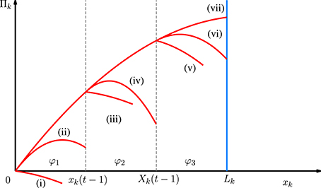
Figure 1. The possible shapes of the profit function of firm k.

FIGURE 2

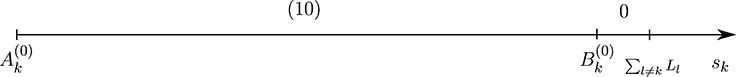
Figure 2. Different segments of R_k when $D_k^{\left(1\right)}\le 0$.

For easier understanding of the different cases notice that $D_1^{\left(0\right)}\ge D_2^{\left(0\right)}\ge D_3^{\left(0\right)}\ge D_4^{\left(0\right)}\ge D_5^{\left(0\right)}$, so if any one of these quantities in non-positive, then the same holds for all others with larger subscripts.

The computation of R_k can be done in the following algorithm:

• Step 1. Set

$\begin{array}{ll}{A}_k^{\left(0\right)}=0,B_k^{\left(0\right)}=\frac{A}{d_k-{\delta }_k}& (21)\end{array}$

Compute $D_k^{\left(l\right)}$ values for l = 1, 2, 3, 4, 5. If all $D_k^{\left(l\right)}$ are non-positive then R_k is determined from Figure 2, otherwise go to next step.

• Step 2. Let $A_k^{\left(1\right)}$ and $B_k^{\left(1\right)}$ be the smaller and larger ones of the roots

$\begin{array}{ll}\frac{A-2x_k\left(t-1\right)\left(d_k-{\delta }_k\right)\pm \sqrt{D_k^{\left(1\right)}}}{2\left(d_k-{\delta }_k\right)}& (22)\end{array}$

If $D_k^{\left(2\right)}\le 0$, then R_k is determined from Figure 3, otherwise go to next step.

• Step 3. Let $A_k^{\left(2\right)}$ and $B_k^{\left(2\right)}$ be the smaller and larger ones of the roots

$\begin{array}{ll}\frac{A-2x_k\left(t-1\right)\left(d_k+{\gamma }_k\right)\pm \sqrt{D_k^{\left(2\right)}}}{2\left(d_k+{\gamma }_k\right)}& (23)\end{array}$

If $D_k^{\left(3\right)}\le 0$, then R_k is determined from Figure 4, otherwise go to next step.

• Step 4. Let $A_k^{\left(3\right)}$ and $B_k^{\left(3\right)}$ be the smaller and larger ones of the roots

$\begin{array}{ll}\frac{A-2X_k\left(t-1\right)\left(d_k+{\gamma }_k\right)\pm \sqrt{D_k^{\left(3\right)}}}{2\left(d_k+{\gamma }_k\right)}& (24)\end{array}$

If $D_k^{\left(4\right)}\le 0$, then R_k is determined from Figure 5, otherwise go to next step.

• Step 5. Let $A_k^{\left(4\right)}$ and $B_k^{\left(4\right)}$ be the smaller and larger ones of the roots

$\begin{array}{ll}\frac{A-2X_k\left(t-1\right)\left(d_k+{\gamma }_k+{\alpha }_k\right)\pm \sqrt{D_k^{\left(4\right)}}}{2\left(d_k+{\gamma }_k+{\alpha }_k\right)}& (25)\end{array}$

If $D_k^{\left(5\right)}\le 0$, then R_k is determined from Figure 6, otherwise go to next step.

• Step 6. Let $A_k^{\left(5\right)}$ and $B_k^{\left(5\right)}$ be the smaller and larger ones of the roots

$\begin{array}{ll}\frac{A-2L_k\left(d_k+{\gamma }_k+{\alpha }_k\right)\pm \sqrt{D_k^{\left(5\right)}}}{2\left(d_k+{\gamma }_k+{\alpha }_k\right)}& (26)\end{array}$

R_k is determined from Figure 7.

FIGURE 3

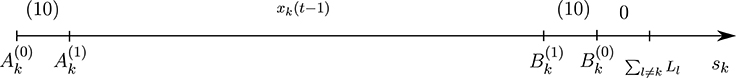
Figure 3. Different segments of R_k when $D_k^{\left(2\right)}\le 0$ and $D_k^{\left(1\right)}>0$.

FIGURE 4

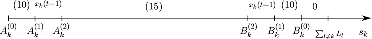
Figure 4. Different segments of R_k when $D_k^{\left(3\right)}\le 0$ and $D_k^{\left(2\right)}>0$.

FIGURE 5

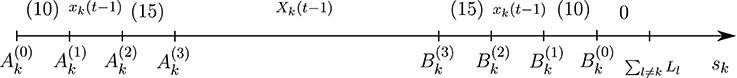
Figure 5. Different segments of R_k when $D_k^{\left(4\right)}\le 0$ and $D_k^{\left(3\right)}>0$.

FIGURE 6

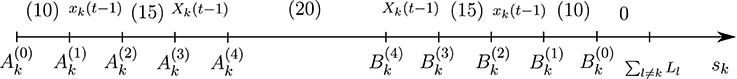
Figure 6. Different segments of R_k when $D_k^{\left(5\right)}\le 0$ and $D_k^{\left(4\right)}>0$.

FIGURE 7

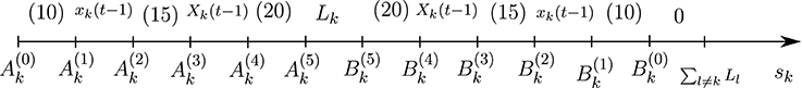
Figure 7. Different segments of R_k when $D_k^{\left(5\right)}>0$.

3. Steady States Analysis

By denoting the best response function of firm k by R_k(s_k, x_k, X_k), the dynamic model with positive adjustment toward best responses can be written as

$\begin{array}{l}{x}_k\left(t\right)=K_k{R}_k\left(s_k\left(t-1\right),x_k\left(t-1\right),X_k\left(t-1\right)\right)\\ +\left(1-K_k\right)x_k\left(t-1\right)\end{array}$

for k = 1, 2, …, n. Clearly a vector $({\overline{x}}_1,\dots ,{\overline{x}}_n,{\overline{s}}_1,\dots ,{\overline{s}}_n,{\overline{X}}_1,\dots ,{\overline{X}}_n)$ is a steady state if and only if for all k,

${\overline{x}}_k=R_k\left({\overline{s}}_k,{\overline{x}}_k{\overline{X}}_k\right)$

${\overline{x}}_k\le {\overline{X}}_k$

and

${\overline{s}}_k={\displaystyle \sum _{l\ne k}}{\overline{x}}_l$

In determining the set of all steady states we have the following possibilities:

(a) ${\overline{x}}_k=0$ if

${\overline{s}}_k\ge \frac{A}{d_k-{\delta }_k}$

(b) ${\overline{x}}_k=L_k$ if

$\begin{array}{ll}\frac{A{\overline{s}}_k}{{\left(L_k+{\overline{s}}_k\right)}^2}-d_k-{\gamma }_k\ge 0& (27)\end{array}$

(c) ${\overline{x}}_k$ is interior if

$\begin{array}{ll}\frac{A{\overline{s}}_k}{{\left({\overline{x}}_k+{\overline{s}}_k\right)}^2}-d_k+{\delta }_k>0>\frac{A{\overline{s}}_k}{{\left({\overline{x}}_k+{\overline{s}}_k\right)}^2}-d_k-{\gamma }_k& (28)\end{array}$

Notice that in case (b), ${\overline{X}}_k=L_k$, so segment of φ₃ is eliminated. The condition of case (b) can be rewritten as

$\begin{array}{ll}{L}_k\le \sqrt{\frac{A{\overline{s}}_k}{d_k+{\gamma }_k}}-{\overline{s}}_k& (29)\end{array}$

and that of case (c) is equivalent to the following:

$\begin{array}{ll}\sqrt{\frac{A{\overline{s}}_k}{d_k+{\gamma }_k}}-{\overline{s}}_k\le {\overline{x}}_k\le \sqrt{\frac{A{\overline{s}}_k}{d_k-{\delta }_k}}-{\overline{s}}_k& (30)\end{array}$

So feasible solution of Inequality (30) for ${\overline{x}}_k$ exists if and only if the right hand side is positive, which occurs if ${\overline{s}}_k<\frac{A}{d_k-{\delta }_k}$, and if the left hand side is below L_k, which is the case when (29) is violated.

Figure 8 illustrates the domain determined by condition (30) for player k, and Figure 9 shows the region of interior steady states in a duopoly.

FIGURE 8

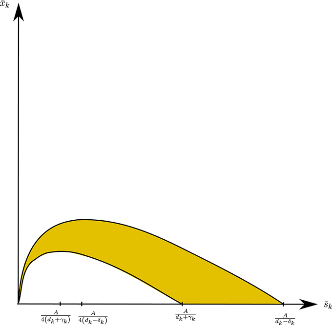
Figure 8. Region of interior steady states components.

FIGURE 9

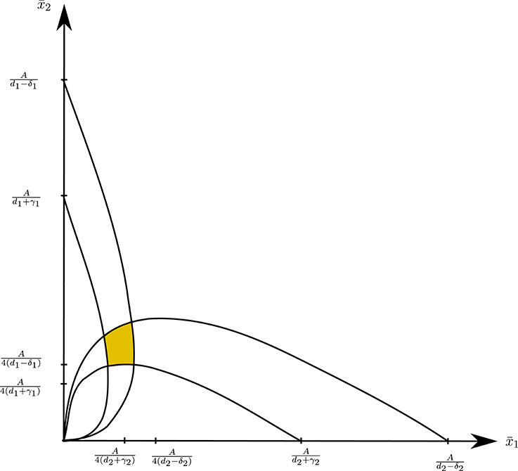
Figure 9. Interior steady states in a duopoly.

4. Simulation Study

The model introduced and analyzed in the previous sections is a clear generalization of the duopoly model of Puu [24, 26, Chapter 7]. His special model can be obtained by selecting α₁ = α₂ = γ₁ = γ₂ = δ₁ = δ₂ = 0 and sufficiently large values of L₁ and L₂. In this particular case, the only fixed point, except the origin, is, of course, the Cournot equilibrium point:

$\{\begin{array}{c}{x}_1^{*}=\frac{d_2}{d_1+d_2}\\ x_2^{*}=\frac{d_1}{d_1+d_2}\end{array}$

In Puu [26] it is proved that whenever one of the ratios of the marginal costs of the duopolists falls outside the interval $\left[3-\sqrt{2},3+\sqrt{2}\right]$, the Cournot point is not stable. Furthermore, the complexity of the dynamics is illustrated considering a bifurcation diagram of firms' output vs. the marginal cost ratio. When we set α₁ = α₂ = γ₁ = γ₂ = δ₁ = δ₂ = 0 and sufficiently large L₁ and L₂, we obtain the bifurcation diagram reported in Figure 10, which is identical to the one presented in Puu [26, p. 271]. This Figure has been obtained with A = 1, c₁ = c₂ = 0, d₁ = 1 and initial condition x₁(0) = x₂(0) = 0.1 when d₂ varies in the interval [5.75, 6.25].

FIGURE 10

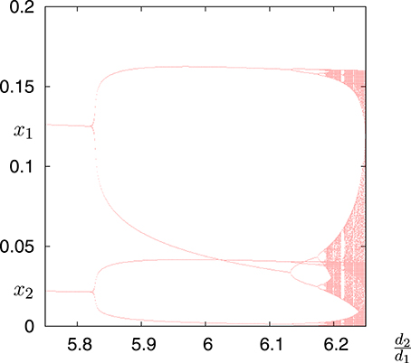
Figure 10. Bifurcation diagram. Amplitudes plotted vs. marginal cost ratio.

The model we present here is much more complex. To understand the effects of the different costs and production constraints we introduced, we analyze each of them separately and compare the dynamics to the one originally presented in Puu [26]. These analyses are reported in Figures 11–14. Each of these figures consists of a bifurcation diagram in the parameter plane (d₂/d₁, α = α₁ = α₂) in which the regions of different periodicity are represented by different colors. Bifurcation diagrams are also shown in which amplitudes are plotted vs. marginal cost ratio as in the original figure in Puu [26, p. 271] which is here reproduced as Figure 10. The two bifurcation diagrams with marginal cost ratio as bifurcation variable help to understand how the different cost coefficients affect the dynamics. Therefore, we will next examine how the dynamic properties of the dynamics depend on the different values of the different cost coefficients. The comparison of these bifurcation diagrams helps to understand the respective roles of isoelastic demand function, workforce flexibility costs and structural limits.

FIGURE 11

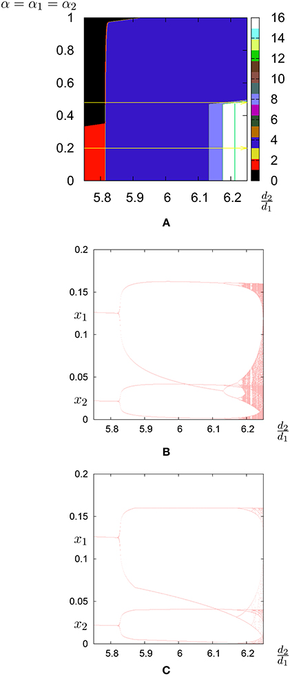
Figure 11. Investment cost. (A) Bifurcation diagram in the parameter plane (d₂/d₁, α = α₁ = α₂); the regions of different periodicity are represented by different colors. The horizontal yellow lines represent the line on which, in (B), the bifurcation diagram is shown with α = α₁ = α₂ = 0.20 and in (C), the bifurcation diagram is shown with α = α₁ = α₂ = 0.48.

Let us start our analysis by considering the effects of the investment costs α_k. As the investment costs are small (Figure 11B) the bifurcation diagram is identical to the case when investment costs are zero. In this case the trajectories after a transient of 5000 iterations are also identical. By contrast, when investments costs are larger (α = α₁ = α₂ = 0.48) the trajectory becomes less complex than in the case of smaller costs (α = α₁ = α₂ = 0.2). This can be explained because larger investment costs dampen firms' reply.

The effects of the hiring costs γ_k are much more pronounced. In fact even for small values of hiring costs the dynamics is much simpler as it can be seen in Figures 12B,C. For even larger values of the hiring costs we do not have cycles as it can be seen from the top of Figure 12A. In this case also, hiring costs dampen firms' reply.

FIGURE 12

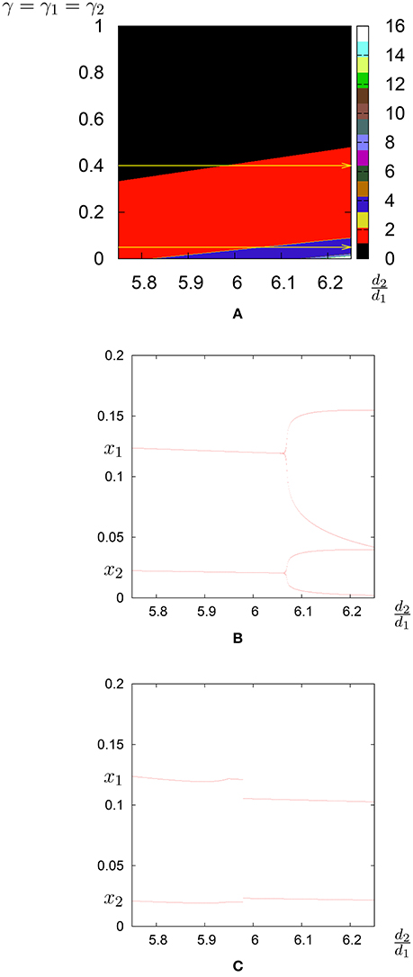
Figure 12. Hiring cost. (A) Bifurcation diagram in the parameter plane (d₂/d₁, γ = γ₁ = γ₂); the regions of different periodicity are represented by different colors. The horizontal yellow line represents the line on which, in (B), the bifurcation diagram is shown with γ = γ₁ = γ₂ = 0.05, and in (C), the bifurcation diagram is shown with γ = γ₁ = γ₂ = 0.4.

When considering layoff costs δ_k, the effects are similar to those of investment costs. For small values of layoff costs the dynamics is similar but not identical to the one with no costs. In fact, although Figures 10, 13C look similar, an inspection of the trajectories after discarding 5000 transient shows some differences. Also in this case, for even larger values of the hiring costs we do not have cycles as it can be seen from the top of Figure 13A. Large enough layoff costs dampen the dynamics.

FIGURE 13

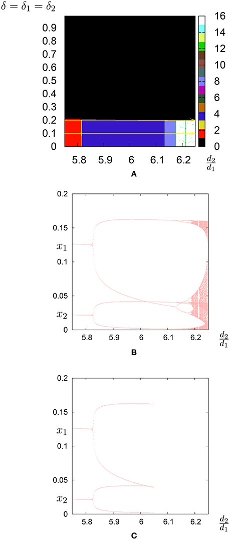
Figure 13. Layoff cost. (A) Bifurcation diagram in the parameter plane (d₂/d₁, δ = δ₁ = δ₂); the regions of different periodicity are represented by different colors. The horizontal yellow lines represent the line on which, in (B), the bifurcation diagram is shown with δ = δ₁ = δ₂ = 0.1 and in (C), the bifurcation diagram is shown with δ = δ₁ = δ₂ = 0.2.

Finally, when considering capacity limits L_k we can see that, unless they are influencing firms' response, they have no effect on the dynamics. As a matter of fact, Figures 10, 14C are identical as they are the respective trajectories after a transient of 5000 iterations. In this case large production limits do not have any effect on the dynamics.

FIGURE 14

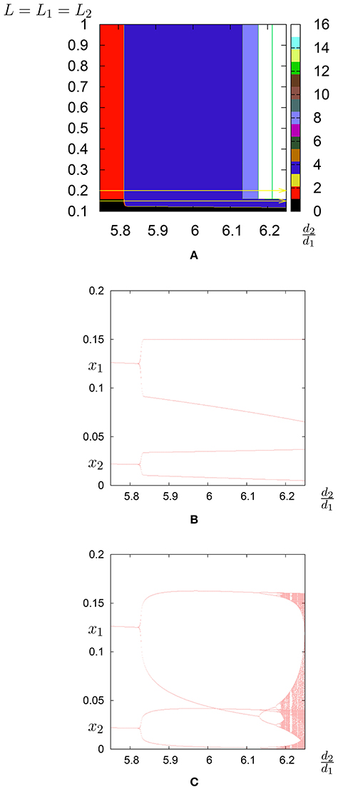
Figure 14. Capacity limit. (A) Bifurcation diagram in the parameter plane (d₂/d₁, L = L₁ = L₂); the regions of different periodicity are represented by different colors. The horizontal yellow line represents the line on which, in (B), the bifurcation diagram is shown with L = L₁ = L₂ = 0.15, and in (C), the bifurcation diagram is shown with L = L₁ = L₂ = 0.2.

5. Conclusions

Non-linear single product oligopolies without product differentiation were introduced and examined where the production cost was linear, and the piecewise linear production adjustment and investment costs made the model non-linear. The non-linearity of the model became even stronger by assuming hyperbolic price function. These models are equivalent with rent-seeking and market-share attraction games as well. The profit functions of the firms are continuous, piece-wise differentiable and strictly concave implying the uniqueness of the best responses. The best response functions of the firms were then determined which are not monotonic in contrast with the case of linear price functions assumed earlier in the literature. The set of all steady states were characterized and illustrated in the case of a duopoly. The asymptotical properties of the steady states were investigated by using simulation. Comparing the dynamics to the one of Puu's original model, showed the different roles these costs have on the dynamics. Although some of them seem to have little effects on the dynamics, others –such as the hiring costs– have a deep impact. In particular, as recruitment and selection cost can be staggering, see for instance Gusdorf [27], they should be considered in order to have a more realistic model. In our analysis these costs make the dynamics less complex than the one predicted by the theoretical model. Furthermore, the dynamics in real word seems to be less complex than the one predicted by models which do not consider these costs. A reason for this discrepancy could be that the hiring costs are high and therefore the dynamics is less complex than predicted.

It will be interesting to consider the case of a generic isoelastic function. Also, further non-linearities can be introduced into the models by assuming non-linear cost functions and different types of the price functions. We will elaborate on these ideas in our next research project.

Author Contributions

UM: Original Idea and Simulations. FS: Mathematical Derivation. AM: General Comments.

Conflict of Interest Statement

The authors declare that the research was conducted in the absence of any commercial or financial relationships that could be construed as a potential conflict of interest.

Acknowledgments

AM has received research grants from the MEXT-Supported Program for the Strategic Research Foundation at Private Universities 2013–2017 and Chuo University (Joint Research Grant). UM has developed this work in the framework of the research project on “Dynamic Models for behavioural economics” financed by DESP-University of Urbino.

References

1. Cournot A. Recherches sur les Principes Mathematiques de la Theorie des Richesses. Paris: Hachette (1838). English translation, Kelly, New York, NY, 1960.

2. Okuguchi K. Expectations and Stability in Oligopoly Models. Berlin; Heidelberg; New York: Springer-Verlag (1976).

Google Scholar

3. Okuguchi K, Szidarovszky F. The Theory of Oligopoly with Multi-product Firms. Berlin; Heidelberg; New York: Springer-Verlag (1999).

Google Scholar

4. Howroyd TD, Rickard JA. Cournot oligopoly and adjustment costs. Econ Lett. (1981) 7:113–7. doi: 10.1016/0165-1765(87)90104-2

CrossRef Full Text | Google Scholar

5. Macleod WB. On adjustment costs and the stability of equilibria. Rev Econ Stud. (1985) 52:575–91. doi: 10.2307/2297733

CrossRef Full Text | Google Scholar

6. Reynolds SS. Capacity investment, preemption and commitment in an infinite horizon model. Int Econ Rev. (1987) 28:69–88. doi: 10.2307/2526860

CrossRef Full Text | Google Scholar

7. Reynolds SS. Dynamic oligopoly with capacity adjustment costs. J Econ Dyn Contl. (1991) 15:491–514. doi: 10.1016/0165-1889(91)90003-J

CrossRef Full Text | Google Scholar

8. Szidarovszky F, Yen J. Dynamic Cournot oligopoly with production adjustment costs. J Math Econ. (1995) 24:95–101. doi: 10.1016/0304-4068(94)00661-S

CrossRef Full Text | Google Scholar

9. Zhao J, Szidarovszky F. N-firm oligopolies with production adjustment costs: best responses and equilibrium. J Econ Behav Organ. (2008) 68:87–99. doi: 10.1016/j.jebo.2007.05.005

CrossRef Full Text | Google Scholar

10. Matsumoto A, Merlone U, Szidarovszky F. Dynamic oligopoly models with production adjustment and investment costs. In: Matsumoto A, Szidarovszky F, Asada T, editors. Essays in Economic Dynamics. Berlin: Springer-Verlag (2016). p. 99–109. doi: 10.1007/978-981-10-1521-2_6

CrossRef Full Text | Google Scholar

11. Matsumoto A, Merlone U, Szidarovszky F. Cartelizing groups in dynamic linear oligopoly with antitrust threshold. Int Game Theory Rev. (2008) 10:399–419. doi: 10.1142/S0219198908002011

CrossRef Full Text | Google Scholar

12. Matsumoto A, Merlone U, Szidarovszky F. Cartelising groups in dynamic hyperbolic oligopoly with antitrust threshold. Aust Econ Papers (2010) 49:289–300. doi: 10.1111/j.1467-8454.2010.00403.x

CrossRef Full Text | Google Scholar

13. Matsumoto A, Merlone U, Szidarovszky F. Dynamic oligopoly with partial cooperation and antitrust threshold. J Econ Behav Organ. (2010) 73:259–72. doi: 10.1016/j.jebo.2009.08.014

CrossRef Full Text | Google Scholar

14. Merlone U, Szidarovszky F. Dynamic oligopolies with contingent workforce and investment costs. Math Comput Simul. (2015) 108:144–54. doi: 10.1016/j.matcom.2014.02.003

CrossRef Full Text | Google Scholar

15. Burr C, Gardini L, Szidarovszky F. Discrete time dynamic oligopolies with adjustment constraints. J Dyn Games (2015) 2:65–87. doi: 10.3934/jdg.2015.2.65

CrossRef Full Text | Google Scholar

16. Tullock G. Efficient rent-seeking. In: Buchanan JM, Tollison RD, Tullock G, editors. Towards a Theory of the Rent-Seeking Society. College Station, TX: Texas A&M Press (1980). p. 97–112.

17. Okuguchi K. Decreasing Returns and Evidence of Nash Equilibrium in Rent-Seeking Games. Mimeo: Department of Economics, Nanzan University, Nagoya, Japan (1995).

18. Szidarovszky F, Okuguchi K. On the existence and uniqueness of pure Nash equilibrium in rent-seeking gams. Games Econ Behav. (1997) 18:135–40. doi: 10.1006/game.1997.0517

CrossRef Full Text | Google Scholar

19. Cooper LG, Nakanishi M. Market-Share Analysis. Dordrecht: Kluver Academic Publisher (1988).

20. Hanssens DM, Parsons LJ, Schultz RL. Market Response Models: Econometric and Time Series Analysis. Dordrecht: Kluver Academic Publisher (1990).

Google Scholar

21. Bischi GI, Chiarella C, Kopel M, Szidarovszky F. Nonlinear Oligopolies: Stability and Bifurcations. Berlin; New York: Springer-Verlag (2010).

Google Scholar

22. Stewart BD, Webster DB, Ahmad S, Matson JO. Mathematical models for developing a flexible workforce. Int J Product Econ. (1997) 36:243–54. doi: 10.1016/0925-5273(94)00033-6

CrossRef Full Text | Google Scholar

23. Nash BJ, Romero J. Flexible workforce: the role of temporary workers in recession and recovery. Region Focus. (2011) First Quarter:21–3, 38. Available online at: https://www.richmondfed.org/~/media/richmondfedorg/publications/research/region_focus/2011/q1/pdf/feature1.pdf

24. Puu T. Chaos in duopoly pricing. Chaos Solitons Fract. (1991) 1:573–81. doi: 10.1016/0960-0779(91)90045-B

CrossRef Full Text | Google Scholar

25. Agliari A, Puu T. A Cournot duopoly with bounded inverse demand function. In: Puu T, Sushko I, editors. Oligopoly Dynamics: Models and Tools. Heidelberg: Springer-Verlag (2002). p. 171–94. doi: 10.1007/978-3-540-24792-0_7

CrossRef Full Text

26. Puu T. Attractors, Bifurcations & Chaos. Nonlinear Phenomena in Economics. 2nd Edn. Berlin; Heidelberg; New York: Springer-Verlag (2003).

Google Scholar

27. Gusdorf ML. Recruitment and Selection: Hiring the Right Person. A Two-Part Learning Module for Undergraduate Students. Alexandria, VA: Society for Human Resource Management (2008).