Disentangling the Information Content of Government Bonds and Credit Default Swaps: An Empirical Analysis on Sovereigns and Banks

1. Introduction

Even though there exists a vast amount of research on the static pricing of complex credit derivatives, such as first-to-default swaps or synthetic collateralized debt obligations (CDOs), there are only a few empirical studies that explore under a dynamic perspective the behavior of sovereign bonds, sovereign credit default swap (CDS), and domestic banks CDS during the last financial downturn. As observed by O'Donoghue et al. [1], investors in bonds, CDS and other simple credit derivatives are exposed to price fluctuations even in the absence of defaults, therefore it is important to analyze the dynamics of these products.

Bond prices and CDS spreads reflect, among other things, in addition to the market risk associated with the dynamics of interest rates, the default risk of the bond issuer and other risks associated with the markets in which these instruments are traded. The use of stochastic multi-factor models allows one to consider information about the entire term structure of bonds and CDS and analyze the frictions caused by the presence of different risks (e.g., market, credit, liquidity, and currency risks), implicit in the behavior of market prices. The purpose of this paper is to use a well-established model from the existing literature to estimate the factors that drive the intensity of default and the different behavior of the markets where these financial instruments are traded. In particular, it is proposed to model: (1) the sovereign credit risk component through a reduced form model calibrated on government bonds; (2) another component, to which we refer to as basis component, estimated by fitting the model on observed sovereign CDS spreads. In the second part of the work, the same methodology is extended to investigate the relationship between sovereign and domestic banking system. In particular, the CDS spreads of major European banks are modeled by considering the common sovereign risk component (obtained from sovereign bond) and an idiosyncratic component driven by the specific risk of the individual bank. For international comparison purposes, the same analysis has been carried out for the main Euro area countries (Italy, Germany, France and Spain).

The multi-factor model here proposed allows us to jointly calibrate the sovereign term structure, the sovereign CDS curve and relations with the domestic banks CDS curve. The approach used in this paper makes possible to explore the dynamics of the different factors influencing the behavior of these market data. The information content of government bonds and credit default swaps is analyzed by considering a unified framework. The entire interest rate and CDS term structures are considered in the calibration exercise.

More in details, we describe a model based on the short-rate process approach first defined in the interest rate context. However, there are two main differences between interest rate and credit derivatives. First, as observed by Cont [2], unlike the interest rate swap, the payoff of a CDS has a binary nature, that is, while the mark-to-market value of a CDS position prior to default may be small, the actual exposure upon default may represent a large fraction of the notional. Second, as outlined by Brigo and El-Bachir [3], while the interest rate derivatives market is one of the most active financial markets with a large number of caps, floors, swaptions and other derivatives, the single-name default swap market presents a very small number of traded derivatives and the calibration of any model with a large number of parameters (for example [4]) becomes unfeasible.

Both the Libor and the swap market models (see [5]) cannot be applied in this context for three main reasons. First these market models have been developed to calibrate the quotes of the most liquid interest rate derivatives traded in the market, that is, caps, floors and swaptions with the purpose of price exotic derivatives, usually traded over the counter, and hedge them. Even if the information derived by the implied volatilities of these liquid derivatives may be considered to capture the market expectation on future rates, the analysis of these derivatives is beyond the scope of this paper. Second, these models are usually calibrated under a static perspective, that is, at each given point in time the model prices have to be as close as possible to the prices traded in the market and, even if the market is quoting unreasonable prices, the trader has to find the parameters that replicate those prices. The trader needs to achieve static consistency in order to provide at each given point in time arbitrage-free prices or to hedge its derivatives portfolio. Conversely, our model is calibrated by following a dynamic approach in order to analyze the long term relations between sovereign term structures, sovereign and banks CDS spreads. Third, only recently, the academia has proposed tractable Libor models with default risk that may be used by practitioners (see [6]), even if probably they are not being used yet, mainly because, as already observed, the single-name credit default markets are not enough liquid to calibrate or estimate any model with a large number of parameters. Our model is calibrated by following a dynamic approach in order to analyze the behavior of yield curves. Under the taxonomy introduced by Nawalkha et al. [7], the model we analyze can be defined as single-plus.

More recently, while most of the empirical studies on this argument are based on the techniques employed in the literature on interest rate term structure models, some authors have proposed modeling the spread log returns. O'Donoghue et al. [1] and Cont and Kan [8] have applied to CDS spreads the techniques commonly employed in modeling stock log returns (see also [9]). Even if this last approach is appealing, in this paper we will implement a classical multi- (instantaneous) factor model. We do not model the dynamics of the risk-free rate. We implicitly assume that the factor driving the interest rate risk is independent on the other risk factors. We model the dynamics of three different types of spreads. First the spread between sovereign bonds and risk-free rates, second the spread between CDS quotes and sovereign bonds, third the spread between bank and sovereign CDS quotes. The aim of this paper is (1) disentangling the credit risk component of sovereign bonds from the interest rate component, (2) exploring the sovereign CDS-bond basis, that is the difference between CDS quotes and sovereign bond yields, and (3) extracting from CDS quote the specific bank credit risk and its relation with the sovereign risk.

Each of these three objectives may have relevant implications from a supervisory perspective. First, disentangling the interest rate and credit risk components of sovereign bond yields allows to properly monitor different risk drivers of banks exposures, which can impact bank solvency in different ways. Second, the treatment of basis risk, i.e., the risk that the relationship between the prices of correlated instruments changes over time, is of material importance to both the standardized and internal model approaches for market risk¹. The basis between bond and CDS curves frequently caused severe losses by banks during adverse periods of stress. Third, disentangling the sovereign and idiosyncratic components of banks credit risk spreads allows to shed light on the sovereign-bank nexus, which has been at the core of the euro area sovereign debt crisis in recent years.

As observed by O'Kane [10], the difference between the German yield and the Libor swap rate with the same maturity may be negative. Even if in this study the reference risk-free rates are the Euribor-swap and the Eonia swap rates, we observe the same empirical fact also for Italy, France and Spain. In view of these empirical facts, we consider the classical Vasicek models extended to a multi-factor framework. This model allows negative values with positive probability and it can capture the patterns observed in market data.

As far as the implementation is concerned, we cast the bond and CDS default term structure into a state-space form and calibrate it with a filter as similarly done by Chen et al. [11], Jarrow et al. [12], Carr and Wu [13], Chen et al. [14], Ang and Longstaff [15], Bianchi and Fabozzi [16], and Li and Zinna [17, 18]. The Kalman filter algorithm together with a maximum likelihood estimation method are considered to fit the model in the period from June 2008 to December 2014. Analytic formulas for the gradient vector and the Hessian matrix of the likelihood function maximized in the optimization algorithm are used, as done in Bianchi and Rocco [19].

The remainder of the paper is organized as follows. Section 2 reviews the Vasicek multi-factor model considered in the empirical study and the ways to computing bond prices, yield levels and CDS spreads. In Section 3 we describe the Bloomberg data about government bonds and the Datastream data about CDS quotes. The estimation algorithms together with the main empirical results are discussed in Sections 4 and 5. Section 6 summarizes the paper main conclusions.

2. The Model

On the lines of Ang and Longstaff [15], we analyze multi-factor Gaussian term structure models under the risk-neutral measure. We assume that the risk neutral dynamics of the default intensities are defined as the sum of Gaussian factors. The dynamics of these underlying factors under the historical measure and the associated market price of risk are left unspecified and they are not investigated. The risk-neutral dynamics are extracted by observed bond yield curves and CDS quotes and we explore both the time-series and cross section dimension. We further assume that the structural parameters are kept constant over time, that is the model proposed is time homogeneous. We point out that the factors driving the intensities are not tradable assets, therefore it is not possible to perform a double-calibration in which the historical and risk-neutral model parameters can be jointly estimated. A joint calibration is possible if both the underlying and the derivative are observable, such as for example for equities and equity options (e.g., [20] for an example of double-calibration). Unfortunately, we cannot estimate actual default probabilities due to the lack of defaults in the data. Therefore, it is not possible to check whether the proposed factor historical dynamics are feasible or not, and for this reason we prefer not to explore these dynamics.

2.1. The Vasicek Process

As proposed by Vasicek [21], a Gaussian Ornstein-Uhlencek (OU) process can be used to model the dynamics of the instantaneous spot rate, that is

$\begin{array}{ll}d{\lambda }_t=\kappa (\eta -{\lambda }_t)dt+\vartheta d{W}_t,& (2.1)\end{array}$

with λ₀ > 0, κ, and ϑ positive parameters, and η ∈ ℝ. Usually, the parameter η is chosen to be positive. We recall that, even if η is not negative, the process can be negative with positive probability (see [5]). Under the Vasicek assumption there exists a closed-form expression for the characteristic function of the integrated process (see Proposition 2.6.2.1 in [22]) and the integral in Equation (2.3) on Section 2.2 can be computed as follows

$\begin{array}{ll}{P}_{Sur\upsilon }^{Vasicek}(\tau >t)=e^{a(t)+b(t){\lambda }_0},& (2.2)\end{array}$

where

$\begin{array}{l}a(t)=-\eta t+\eta \frac{1-e^{-\kappa t}}{\kappa }-\frac{{\vartheta }^2}{4{\kappa }^3}{\left(1-e^{-\kappa t}\right)}^2\\ +\frac{{\vartheta }^2}{2{\kappa }^2}\left(t-\frac{1-e^{-\kappa t}}{\kappa }\right),\\ b(t)=-\frac{1-e^{-\kappa t}}{\kappa }.\end{array}$

It follows that the yield is

$y(0,t)=-\frac{1}{t}\left(a(t)+b(t){\lambda }_0\right).$

In this paper, the Vasicek factor will be used in a multivariate framework, as described in Section 2.3.

2.2. Evaluate CDS Spreads

We consider a reduced-form approach to model the default probability, and we assume that the default intensity is a stochastic process (see [23]). There is a general consensus in assuming a stochastic intensity instead of a deterministic intensity to model uncertainty about the future dynamics of the credit risk of a given reference entity. A similar framework has been used to price interest rate derivatives, and it can be used to model the risk-free curve. As we will briefly describe in the following, in the credit derivatives case one models the default intensity process while in the interest rate case one models the spot rate or the factors explaining the term structure. More in detail, in a reduced-form model one assumes that the time of default is determined by the first jump time of a Cox process N_t starting from zero and with a stochastic intensity rate λ_t, where 0 ≤ t ≤ T. Under this setting the default time τ is defined as

$\tau =\inf \left\{t>0|N_t>0\right\}=\inf \left\{t>0|I_t>E_1\right\},$

where the process I_t is usually defined as an integrated process, i.e.,

$I_t={\displaystyle {\int }_0^t{\lambda }_s}ds$

where λ_t is often a stationary affine process and E₁ is an exponential random variable with mean equal to 1. It follows that the survival probability up to time t is equal to

$\begin{array}{ll}{P}_{Sur\upsilon }(\tau >t)=E\left[\exp (-I_t)\right]={\varphi }_{I_t}(i),& (2.3)\end{array}$

where ϕ_It(u), with u ∈ ℝ, is the characteristic function relative to I_t and i is the imaginary unit². We remind that the characteristic function of a random variable X is defined as

${\varphi }_X(u)=E\left[\exp (iuX)\right],$

where u ∈ ℝ. By assuming a model for the intensity process λ_t we can compute the corresponding survival probability. If one knows the characteristic function of the process I_t, it is straightforward to compute the expectation in Equation (2.3).

Following the computations reported in O'Kane and Turnbull [24], given a model for the survival probability, the fair spread of a CDS expiring at time T is

$\begin{array}{l}{c}_T^{CDS}\\ =\frac{(1-R){\displaystyle {\sum }_i^{n}D(0,t_i)}(P_{Sur\upsilon }(t_{i-1})-P_{Sur\upsilon }(t_i))}{{\displaystyle {\sum }_i^{n}D(0,t_i)}{P}_{Sur\upsilon }(t_i)\Delta t_i+\frac{1}{2}{\displaystyle {\sum }_i^{n}D(0,t_i)}(P_{Sur\upsilon }(t_{i-1})-P_{Sur\upsilon }(t_i))\Delta t_i},& (2.4)\end{array}$

where R is the recovery rate (usually assumed equal to 40 per cent), D(0, t) is the discount factor, t₁, … , t_n = T represent the dates of payment at the end of each period t_i until maturity T.³ Fee and loss payments are assumed to be made at the end of each period. Furthermore, it is taken into account that if default occurs between some payment dates, the fee has to be paid only for the portion between the last payment date and the time of default as the insurance buyer is protected only for that period.

In this paper, to calibrate the model instead of directly considering the formula in Equation (2.4) as done in Bianchi and Fabozzi [16], we bootstrap the default probability curves from CDS market quotes. That is, for each given point in time and for each maturity, after having fixed a constant recovery rate (we assume 40 per cent for both sovereign and bank CDS), we find the constant default intensity λ such that the CDS quote coincides with the right-hand side of the equality (2.4). We then calibrate the proposed model on these default probability curves. Since these curves can be expressed as a linear function of the state variables (i.e., unobservable factors) we will use a maximum likelihood estimation method based on the Kalman filter algorithm as proposed in Bianchi and Rocco [19].

2.3. A Multi-factor Reduced-Form Model

The extension of Equation (2.3) to the sum of two or more default intensity factors ${\lambda }_t^1$, … , ${\lambda }_t^n$ is straightforward when pairwise independence is assumed between factors. The formula in Equation (2.3) becomes

$\begin{array}{ll}{P}_{Sur\upsilon }(\tau >t)={\varphi }_{I_t^1}(i)\cdots {\varphi }_{I_t^n}(i).& (2.5)\end{array}$

However, if one considers dependent factors, the decomposition in Equation (2.5) no longer holds. Normal-based models may still have a closed-form solution, but in general, if one assumes a richer dependence structure (for example, a multivariate model or a copula allowing for tail dependence), Monte Carlo simulations or numerical methods are needed to evaluate the survival probability. The assumption of independence is often used in the literature. For instance, Feldhütter and Lando [26] proposed a model with six independent factors to calibrate Treasury bonds, corporate bonds, and swap rates using both cross-sectional and time-series properties of the observed yields. This independence assumption may be restrictive (see [27]), although the advantage is that pricing formulas have explicit solutions, and the model is more parsimonious with fewer parameters to estimate (see also [15]). By following a similar approach, in our empirical analysis we will consider a multi-factor model with independent Vasicek factors. As obeserved in Bianchi and Rocco [19], this assumption allows us to maintain both computational tractability and model flexibility.

In order to calibrate (1) the sovereign yield curve, obtained from the prices of sovereign bonds, (2) the sovereign CDS curve, obtained from the spreads of sovereign CDS, and (3) the banks CDS curve, obtained from the spreads of bank CDS, we implement in three different ways a multi-factor model.

We assume that the discount (risk-free) factor satisfies the following equality

$\begin{array}{ll}D(0,t)=𝔼[e^{-{\displaystyle {\int }_0^t{r}_s}ds}]& (2.6)\end{array}$

where r_t is a short-rate process and the price of a defaultable zero-coupon bond can be written as

$\begin{array}{ll}B(0,t)=𝔼[e^{-{\displaystyle {\int }_0^t\left(r_s+(1-R){\delta }_s\right)}ds}]& (2.7)\end{array}$

where R is the recovery rate. We assume that the processes r_t and δ_t are independent, and it follows that

$\begin{array}{l}{y}_{bond}(0,t)-y_{risk-free}(0,t)=-\frac{1}{t}\log \left(𝔼[e^{-{\displaystyle {\int }_0^t(1-R)}{\delta }_{s}ds}]\right)\\ =-\frac{1-R}{t}\left(A(t)+B(t){\lambda }_0\right)& (2.8)\end{array}$

where A(t) and B(t) are matrices that can be derived by considering the affine structure of the proposed model. This means that the model can be directly calibrated by considering the spread between the risky sovereign bond yield and the risk-free bond yield, without calibrating a model for the risk-free yield. Therefore, we calibrate the model on the observed spread between the sovereign yield curve and the risk-free one. More precisely, we define the default intensity process δ_t as

$\begin{array}{ll}{\delta }_t={\lambda }_t^1+{\lambda }_t^2,& (2.9)\end{array}$

where ${\lambda }_t^1$ and ${\lambda }_t^2$ are two independent Vasicek factors. By extending the model in Equation (2.7), it is possible to define the survival probability to be used to evaluate CDS spreads (both sovereign and banks CDS spreads), that is

$\begin{array}{ll}{P}_{Sur\upsilon }(\tau >t)=E\left[\exp \left(-{\displaystyle {\int }_0^t\left({\delta }_s+{\xi }_s\right)}ds\right)\right],& (2.10)\end{array}$

where δ_s is define in Equation (2.9), and ξ_t is an additional component which measures the difference between bond prices and CDS spreads. We assume that

$\begin{array}{ll}{\xi }_t={\lambda }_t^3+{\lambda }_t^4,& (2.11)\end{array}$

where ${\lambda }_t^3$ and ${\lambda }_t^4$ are two independent Vasicek factors, and that the Brownian motions driving ${\lambda }_t^i$, with i from 1 to 4 are mutually independent. The model (2.10) will be used to calibrate both sovereign and bank CDS spreads. As in Equation (2.8) the factor ξ_t, can be calibrated without considering the risk-free factor, that is, by assuming that the processes δ_t and ξ_t are independent, it follows that

$\begin{array}{l}{y}_{cds}(0,t)-y_{risk-free}(0,t)=-\frac{1}{t}\log \left(𝔼[e^{-{\displaystyle {\int }_0^t(1-R)({\delta }_s+{\xi }_s)}ds}]\right)\\ =-\frac{1-R}{t}\left(A^{\prime }(t)+B^{\prime }(t){\lambda }_0\right).& (2.12)\end{array}$

where A′(t) and B′(t) are matrices that can be derived by considering the affine structure of the proposed model. A further enhancement is given by the following approach, that is, the survival probability to be used to evaluate bank CDS spreads is assumed to be as follows

$\begin{array}{ll}{P}_{Sur\upsilon }(\tau >t)=E\left[\exp \left(-{\displaystyle {\int }_0^t\left({\delta }_s+{\xi }_s+{\gamma }_s\right)}ds\right)\right],& (2.13)\end{array}$

where δ_s is defined in Equation (2.9), ξ_t in Equation (2.11), and γ_t is

$\begin{array}{ll}{\gamma }_t={\lambda }_t^5+{\lambda }_t^6,& (2.14)\end{array}$

where γ_t is an additional component which measures the difference between sovereign and domestic bank CDS spreads. Also in this extension, we assume that ${\lambda }_t^5$ and ${\lambda }_t^6$ are two independent Vasicek factors, and that the Brownian motions driving ${\lambda }_t^i$, with i from 1 to 6 are mutually independent. We point out that, under the independence assumption we consider, the integrals Equations (2.7), (2.10), and (2.13) have a close-form solution. In order to model possible negative differences between sovereign and risk-free rates, and between sovereign and banks CDS spreads, and to reduce the calibration error, in our empirical study we assume that η is zero for the factors ${\lambda }_t^2$, ${\lambda }_t^4$ and ${\lambda }_t^6$. This last assumption is needed to avoid overparametrization problems that may affect the calibration performance.

3. The Data

This section provides a description of the data used in the empirical analysis. We obtained from Bloomberg Italian, French, German, and Spanish bond term structure data from June 30, 2008 to December 31, 2014. For Spain we consider only bonds with maturities larger than 2 years, because for shorter maturities Bloomberg does not provide data until the second semester of 2011. The time period in this study includes (1) the high volatility period after the Lehman Brothers filling for Chapter 11 bankruptcy protection (September 15, 2008), (2) the recent sovereign debt crisis, during which the spread between the 10-year Italian BTP and the German bund exceeded 500 basis points (bp), and (3) the assumption by the European Central Bank (ECB) of responsibility for the direct supervision of the major euro-area banks. The risk-free zero rates are bootstrapped from the Euribor rate for short-term maturities up to 9 months and the EU swap curve for maturities from 1 to 30 years. For each observation day and for each maturity, the observed discount factor is computed by linear interpolation of the zero rates term structure. The same procedure is considered to find the risk-free rates starting from the Eonia swap data. We refer to these rates as risk-free Euribor-swap and risk-free Eonia, respectively. In our analysis, we will consider both rates as discount factors. As shown in Figure 1, the Euribor-OIS basis explosion of 2008 and between the end of 2011 and the beginning of 2012 is essentially a consequence of the different credit and liquidity risk reflected by Euribor-swap and Eonia swap rates (see [28] for more detail on this aspects). Even if many banks now consider Eonia swap rates as the risk-free rate when collateralized portfolios are valued and XIBOR for this purpose when portfolios are not collateralized, Hull and White [29] have suggested to use Eonia swap rates in all situations.

FIGURE 1

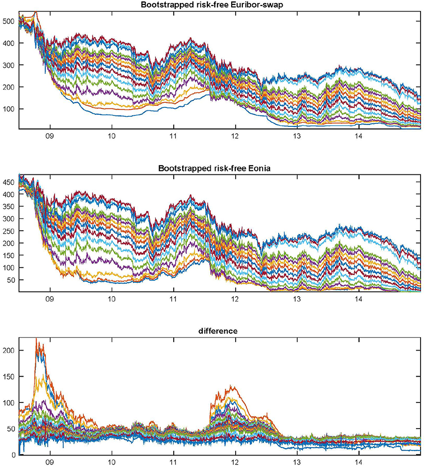
Figure 1. Bootstrapped zero rates form the Euribor and swap curve and Eonia swap curve from June 30, 2008 to December 31, 2014. The zero rates and their difference range from the 3-month to the 30-year maturity.

Furthermore, we observe that the differences between sovereign and risk-free rates (both Euribor-swap and Eonia) may be negative, particularly at the end of 2008 and for the shortest maturities.

In addition to sovereign CDS data (in US dollar), we consider CDS spread data (in Euro) of seven Italian banks: Banco Popolare (BP), Unione di Banche Italiane Scpa (UBI), Banca Popolare di Milano (PMI), Mediobanca (MB), Banca Monte Paschi di Siena (BMPS), Intesa San Paolo (ISP), e Unicredit Group (UCG). Then we consider CDS spread data (in Euro) of 14 major European banks together with the corresponding sovereign bond and CDS term structure data. We analyze for the Germany, Deutsche Bank (DBK), Commerzbank (CBK), Bayerishe Landesbank (BLGZ), Landesbank Baden-Wüttember (LBS), Norddeutsche Landesbank Girozentrale (NLB), and HSH Nordbank (NSH); for the France, BNP Paribas (BNP), Société Générale (GLE), Crédit Agricole Group (ACA), Natixis (KN); finally, for the Spain, Banco Santander (SAN), BBVA, Banco de Sabadell (SAB), and Banco Popular Espanol (POP).

Mid spreads for maturities 1, 3, 5, 7, and 10 years are obtained from Thomson Reuters Datastream from June 30, 2008 to December 31, 2014. Italian, French, German and Spanish sovereign CDS spreads in US dollar for the same maturities are also obtained from Thomson Reuters Datastream. In Table 1 we report some summary statistics for the 5-year CDS quotes. We are aware of the fact that (1) CDS data refer to market quotes, not necessarily realized in actual transactions, (2) the collected bid-ask difference could not reflect the real liquidity of the market, (3) the data can be different among data providers, as recently observed by Mayordomo et al. [30], and, furthermore, (4) the transactions generally involve the 5-year maturity contracts as described in Amadei et al. [31].

TABLE 1

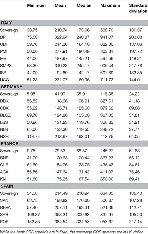
Table 1. Summary statistics of the CDS spreads with maturity 5 year between June 30, 2008 and December 31, 2014 for the four sovereign and the 21 banks considered in the empirical study.

In Figure 2 we report the time-series from January 2, 2006 to December 31, 2014 of the 5-year Italy CDS spread and the implied CDS spread with the same 5-year maturity. This difference represents the so-called CDS-bond basis, that is

$\begin{array}{ll}Basi{s}_t^i=c_{t,T_i}^{CDS}-c_{t,T_i}^{impliedCDS}& (3.1)\end{array}$

where $c_{t,T_i}^{CDS}$ is the spread at time t of the CDS with maturity T_i, and $c_{t,T_i}^{impliedCDS}$ is the spread computed as the difference between the yield at time t of the bond with maturity T_i and the Eonia swap rate at time t with maturity T_i. As observed in Amadei et al. [31] and shown in Figure 2, the basis is almost always positive. However, it is around zero in periods of calm.

FIGURE 2

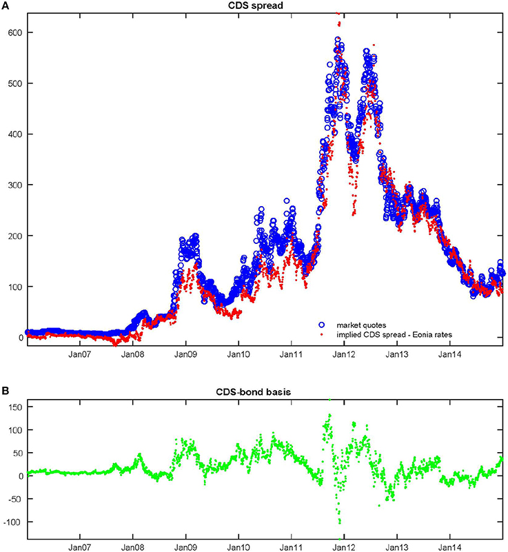
Figure 2. Observed 5-year CDS spread, implied 5-year CDS spread and 5-year CDS-bond basis from January 02, 2006 to December 31, 2014. We report (A) the observed Italian 5-year CDS spread, the implied 5-year CDS spread computed as difference between the observed Italian 5-year bond yield and the 5-year Eonia swap rate; (B) the 5-year CDS-bond basis, that is the difference between the observed CDS spread and the implied one.

4. Fitting Market Data in Practice

Pan and Singleton [32] observed that the use of a stochastic interest rate model does not improve the estimates significantly. For this reason we do not calibrate the risk-free term structure. Alternatively, by assuming the model in Equation (2.6), the stochastic risk-free component r_t may be calibrated by fitting the zero rates term structure based on the Euribor rate and the EU swap curve or on the Eonia swap curve. To summarize, the calibration exercise is divided into four main steps (each of them is repeated using alternatively Euribor and swap rates, or Eonia swap rates as risk-free rates).

1. We bootstrap the risk-free zero curve from market rates and compute the spread between sovereign bond yield and the risk-free zero curve. Then, using the risk-free curve, we bootstrap the survival probabilities from the CDS quotes (both sovereigns and banks).

2. We calibrate δ_t (two Vasicek factors) based on the spread computed in the previous step.

3. Given an estimate for δ_t, ${\xi }_t^{soʋ}$ (two Vasicek factors) can be calibrated on the sovereign CDS spreads; in this case ${\xi }_t^{soʋ}$ represents the difference between the credit risk implied by market CDS spreads and bonds yields. This factor can capture the CDS-bond basis defined in Equation (3.1) and shown in Figure 2. The factor ${\xi }_t^{soʋ}$ can be viewed as the instantaneous CDS-bond basis. As discussed in Section 5.2, this difference may be caused by a different liquidity between the two markets, the counterparty risk in the CDS spreads, possible other risk factors associated with the market microstructure.

4a. Given an estimate for δ_t, ${\xi }_t^i$ (two Vasicek factors) can be calibrated on the CDS spreads of a domestic bank i; in this case ${\xi }_t^i$ represents the difference between the credit risk implied by the sovereign bond yields and the risks reflected in bank CDS spreads. This difference can be viewed as a specific risk and it may include the idiosyncratic credit risk of the reference entity, a liquidity component, and possible other risk factors associated with the market microstructure.

4b. In the extension of the model presented in Equation (2.13), step 4a is replaced by the following. Given an estimate for both δ_t and ${\xi }_t^{soʋ}$, calibrated on the sovereign bond term structure and on the corresponding sovereign CDS spreads, ${\gamma }_t^i$ can be calibrated on the CDS spreads of a domestic bank i; in this case,γ_t represents the difference between the bank CDS spreads and the corresponding sovereign CDS spreads.

There are two possible methodologies to estimate a reduced-form model: (1) one can fit the model to the daily spreads observed in the market and check both the model capabilities and the parameter stability; or (2) one can extract the unobservable default intensity process (or processes) by using a filter as described by Lando [33] and empirically tested by Jarrow et al. [12]. We will consider the second approach. In all the cases we are interested in, the model can be written in the following form

$\begin{array}{l}{x}_t=f(x_{t-1},\Theta ,{\upsilon }_{t-1})\\ z_t=h(x_t,\Theta ,{\epsilon }_t)& (4.1)\end{array}$

where t is the day counter, x_t is the state variable (also referred to as the latent or unobservable factor) and it can be also a multidimensional variable, as in our case, v_t−1 is the randomness from the state variable and Θ are the model parameters. The state variable follows the dynamics described by f. The variable z_t represents the set of observations, in our case the difference between sovereign bond yields and risk-free rates (or between CDS spreads and sovereign bond yields) observed in the market. Then, the function h is the so-called measurement function, which in our case is given by the bond (or the CDS) spread pricing formula, and it depends on the state variable, model parameters and measurement noise ε_t. A standard hypothesis assumes that this measurement noise is normally distributed: since we consider more than one yield (or more than one CDS spread) observations each day, we have a multivariate normally distributed error. Even though the measurement error covariance matrix R can be set as a non-diagonal matrix, it is chosen to be diagonal in this study and therefore the covariance structure of the factors is represented only by the model itself and not by the measurement error covariance matrix. Since the model proposed in Equation (4.1) is Gaussian with respect to the state variable and linear with respect to the measurement function, the classical Kalman filter can be used. More details on the maximum likelihood estimation (MLE) method implemented to calibrate market data can be found in Bianchi and Rocco [19]. In the algorithm proposed by Bianchi and Rocco [19] the gradient and the Hessian of the likelihood function involved in the optimization problem can be computed in closed form. As already observed the similarities between the algorithms used to dynamically calibrate the bond term structure and the CDS spreads come from the fact that the formula to price a bond given in Equation (2.7) is similar to the formula to compute the survival probability given in Equations (2.10) and (2.13).

5. The Empirical Analysis

In this section we report the estimation results of the calibration conducted on sovereign bonds and on sovereign and bank CDS quotes. In Section 5.1 we empirically analyze the spread between sovereign bonds and risk-free rates. Then, in Section 5.2, we study the dynamics of the CDS-bond basis and, finally, we evaluate the specific bank credit risk component extracted from bank CDS quotes in Section 5.3.

In order to avoid strange patterns in the optimization algorithm, we constrain the parameters (κ, η, ϑ) of each Vasicek factor to range in the region between (1e-3, 1e-3, 1e-3) and (10, 0.1, 0.25). These values seem to be reasonable for the model we are considering and the data we are analyzing: the long term mean η and the volatility ϑ cannot be too high; the boundaries for the speed of mean reversion κ are wide enough to explain different possible dynamics. As can be observed in the following Tables 5–10, the optimal value parameter η sometimes hits the boundaries of the selected parameters region (i.e., η is equal to 0.1). This may be due to an overparametrization problem. Furthermore, after some preliminary empirical tests, we observed that enlarging the boundaries does not improve the calibration procedure. The parameter σ_ε (i.e., the standard deviation of the measurement noise) ranges between 1e-3 and 0.5. As done in Bianchi and Rocco [19], the optimization algorithm applied in this study is the sequential quadratic programming method implemented in the fmincon Matlab function in which the option sqp is selected. The analytic gradient vector of the likelihood is provided in order to speed up the algorithm. As an alternative the interior point algorithm that considers the analytic Hessian matrix can be used. We point out that the computation of the analytic Hessian is time consuming, and for this reason we choose to use it only to compute the standard errors of the parameters and not to include it into the optimization algorithm. As starting point of the algorithm we select a random point in the parameter region. First we calibrate the model on the data that considers the Euribor-swap rates as risk-free rates, then we select the optimal parameters of this calibration as starting point of the calibration on the data considers the Eonia rates as risk-free rates.

For comparative purposes, the models performance across maturities and different observations days are evaluated by the root mean square error (RMSE)

$\begin{array}{ll}RMSE=\sqrt{{\displaystyle \sum _t{\displaystyle \sum _{T_i}\frac{{(c_{t,T_i}^{market}-c_{t,T_i}^{model}(\Theta ))}^2}{\text{number of observations}}}}},& (5.1)\end{array}$

where $c_{t,T_i}^{market}$ refers to the observed data (bond spreads with respect to risk-free zero-rates and CDS spreads with respect to bond yields) with maturity T_i observed at time t and $c_{t,T_i}^{model}(\Theta )$ are the model estimates.

5.1. The Sovereign Bond Spread

We observe that sometimes may happen that the defaultable zero rates extracted from sovereign bonds are smaller than the zero rates bootstrapped from Euribor-swap rates (i.e., the spread represented by the factor δ_t may be negative). This means that the risk implied in the market quotes of sovereign debt is smaller that the risk of the rate commonly used as discount factor in derivatives pricing. This phenomenon is well-known and there is a lively debate among academics and quants. Even if it may be caused by the counterparty and the liquidity risks in the interbank and interest rate derivatives market, there is not yet a general consensus on which model to use and on which discount rate to consider to price defaultable bonds and derivatives. As already observed, in 2008 the Euribor-OIS spread, that is the difference between the Euro interbank offered rate (Euribor) and the overnight indexed swap (OIS), reached unprecedented levels. This spread is a measure of both credit and liquidity risk. Morevover, on September 17, 2008, Bloomberg reported that there was a flight to safety as investors sold off their positions in credit risky assets and invested those funds in short-term Treasury bills, resulting in Treasury bills rates falling to their lowest level since World War II. A similar investor behavior was observed in Europe. For this reason we will consider also the model that take into consideration the risk-free zero rates bootstrapped from the Eonia swap curve. However, even if the Eonia rates are generally smaller that Euribor-swap rates, as shown in Figure 1, it may also happen that defaultable zero rates extracted form sovereign bonds are smaller than the zero rates bootstrapped from Eonia swap rates.

In Tables 2 and 5 we report, for each country and each maturity, the sovereign bond spread term structure calibration error and the corresponding estimated parameters in the period from January 03, 2008 to December 31, 2014 based on the multi-factor reduced form model described in Section 2.3. In Table 6 we report the estimated parameters by considering the risk-free Eonia rates. Then, in Figure 3 the estimated Italian spreads are compared with those observed in the market⁴. As shown in Table 2, the overall RMSE across all maturities ranges from 9.45 bp for Germany to 23.21 for Italy (11.50 bp for France to 22.37 for Italy when considering the risk-free Eonia). The countries reporting the smallest calibration error are Germany, if one considers the spread with respect to the Euribor-swap rate, and its RMSE ranges from 6.66 bp for the 6-year maturity to 13.01 bp for the 30-year maturity, and France, if one considers the spread with respect to the Eonia rate, and its RMSE ranges from 9.50 bp for the 1-year maturity to 14.34 bp for the 20-year maturity. The country reporting the largest calibration error is Italy, and the RMSE ranges from 18.46 bp for the 6-year maturity to 30.48 bp for the 2-year maturity, and if one considers the spread with respect to the Eonia rate it ranges from 16.92 bp for the 6-year maturity to 30.71 bp for the 2-year maturity. The RMSE values reported in Table 2 show that the calibration error depends on the maturity. However, based on the RMSE values, the model performance is satisfactory.

TABLE 2

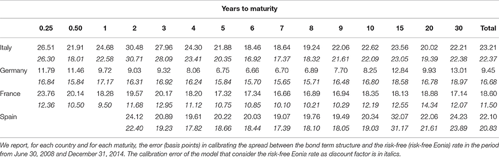
Table 2. Calibration error of the 2-factor Vasicek model.

FIGURE 3

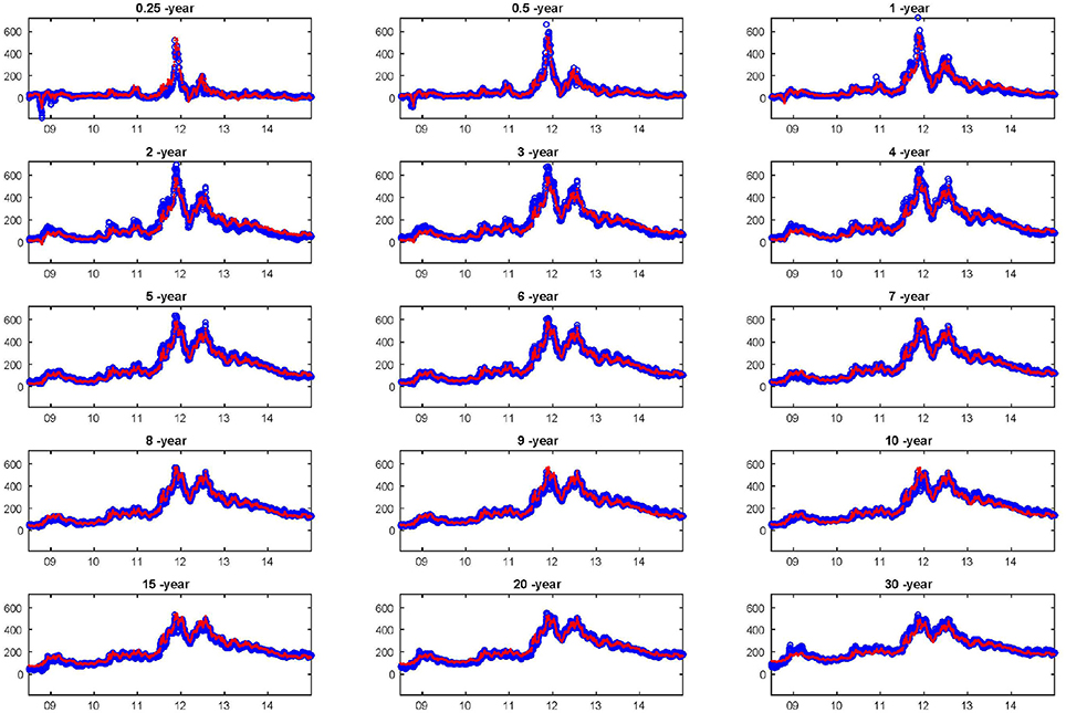
Figure 3. Calibration of the 2-factor default intensity process δ_t on the Italy bond yields from January 02, 2008 to December 31, 2014. We report the observed spreads between bond and risk-free rates and the estimated ones for all maturities investigated. The Kalman filter is considered to extract the unobservable default intensity processes.

In Tables 5, 6 we report the estimated parameters, the corresponding value of the gradient and the square of the standard errors. The value of the likelihood and of the first order optimality condition at the optimal point is also shown. For the definition of the first order optimality condition we refer to the Matlab documentation.

Then in Figure 4 we show the dynamics of the estimated instantaneous default intensity, that is the trajectory of the process δ_t. This default intensity does not represent the overall country risk, but only the specific default risk component. We consider both risk-free Euribor-swap (in blue) and risk-free Eonia (in red) rates as discount factor. The two trajectories differ only slightly. Even if the long term mean of the process is strictly positive, the process becomes negative. This is mainly caused by the fact that the difference between the sovereign yield and the selected risk-free rate may become negative or very close to zero. During the period of turmoil, the intensity sharply increases: this is the case for Italy and Spain. In calm periods, the instantaneous default intensity is close to zero, that is the short-term country risk is negligible. Note that for Spain the estimation results may be affected by the fact that we do not have data for maturities smaller than 2 years.

FIGURE 4

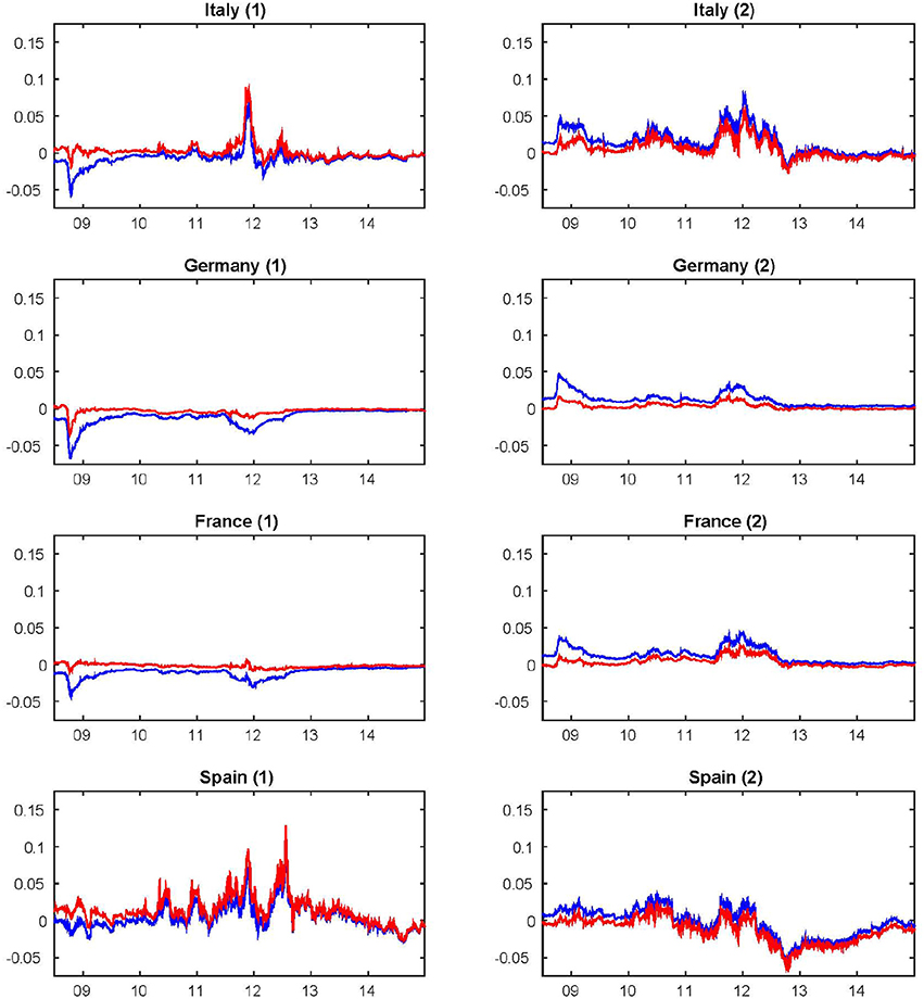
Figure 4. Default intensity processes based the multi-factor model with Vasicek dynamics for the four sovereigns from June 30, 2008 to December 31, 2014. The Kalman filter is considered to extract the unobservable default intensity processes δ_t (1) and ${\xi }_t^{soʋ}$ (2). While in (1) we report the estimation of the factor driving the spread between the sovereign bond yield and the risk-free rate, in (2) we report the estimation of the factor driving the CDS-bond basis. We consider both risk-free Euribor-swap (in blue) and risk-free Eonia (in red) rates as discount factor.

As observed by Ang and Longstaff [15], the value of δ_t essentially captures the level of the shortest maturity spread while the parameters κ, η, and ϑ capture the average slope and curvature of the term structure throughout the sample period. This in practice means that δ_t represents the short-term country specific risk.

5.2. The Time-Varying CDS-Bond Basis

As done in other similar studies (see [18]) we assume that euro-denominated CDS spreads are equal to dollar-denominated CDS spreads. For European sovereign entities the contracts denominated in US dollars are generally more liquid than the contracts denominated in euros, as the former protect the investor against the risk of euro depreciation in the event of default. However, possible currency effect are captured by the factor ξ_t. This means that the dynamics of the CDS-bond basis may be affected by the fact that we are investigating US dollar denominated CDS spreads.

In Figure 2 we report the time-series of the 5-year Italian CDS-bond basis. As observed by Amadei et al. [31], government bonds of the main European countries show almost always a positive basis, and only in the case of Greece there have been persistent negative basis episodes. As discusses by Lando [33] and Haworth et al. [34], even for corporate entities the basis has been rarely close to zero. A variety of different supply and demand, liquidity and technical factors may cause short-term distortions between the cash and CDS markets. Among other factors, a CDS spread cannot become negative while the spread over XIBOR for a high quality issuer can be negative. We refer to Ang and Longstaff [35] for a detailed discussion on this topic.

In this section we assume that the sovereign CDS default intensity has the following form

$x_t^{so\upsilon }={\lambda }_t^1+{\lambda }_t^2+{\lambda }_t^3+{\lambda }_t^4={\delta }_t+{\xi }_t^{so\upsilon },$

where the first two factors (${\lambda }_t^1$ and ${\lambda }_t^2$) have been estimated in the previous Section 5.1. The factor ${\xi }_t^{soʋ}$ is allowed to be negative in order to give more flexibility in the calibration exercise, while the long term mean of the default process ${\xi }_t^{soʋ}$ remains positive. As already observed, also in this case the KF method is used to perform the state and parameter estimation, to extract ${\xi }_t^{soʋ}$, and to find its parameters from the cross-section of sovereign CDS spreads over the observation period. This approach allows one to divide the estimation exercise into two steps: (1) δ_t is estimated by considering the whole sovereign bond term structure over time (see Section 5.1); (2) the basis factor (i.e., ${\xi }_t^{soʋ}$) is extracted by taking into consideration the estimate of δ_t together with the observed sovereign CDS quotes.

The country reporting the smallest calibration error is France. For this country the overall RMSE is 6.72 (6.77) if one considers the Euribor-swap (Eonia) rate as discount factor. The country reporting the largest calibration error is Italy, with the overall RMSE equal to 18.28 (20.01), if one considers the spread with respect to the Euribor-swap (Eonia) rate.

In Tables 5, 6 we report the estimated parameters of the Vasicek factor ξ_t, representing the instantaneous basis. The parameter η₁, representing the mean-reverting level is positive, that is, the instantaneous Italian CDS-bond basis is positive on the long term, even if it can become negative in particular market conditions. A similar result has been obtained for all other countries considered.

In Figure 4 we report the estimated instantaneous basis ξ_t calibrated on the difference between CDS quotes and bond yields. We note that the dynamics of this process may be partially affected by the fact that while the sovereign term structure ranges from 3-month to 30-year, the CDS curve has only five maturities (1-, 3-, 5-, 7- and 10-year). Recall that for other maturities the CDS are illiquid or not traded. This intensity does not represents the overall country risk, but only the specific basis component. We note that these dynamics vary across countries, and they depend on the selected discount factor. Considering both risk-free Euribor-swap (in blue) and risk-free Eonia (in red) rates as discount factor, the difference between the two trajectories is very limited. The trajectory of the instantaneous basis of Italy and Spain is more volatile compared to those of Germany and France. For these last countries the basis is closed to zero, particularly when the risk-free Eonia rate is used as discount factor. In the last 2 years (2013–2014) also for Italy the short-term basis risk has been hovering around zero.

We observe that in the estimation of the basis factor (${\xi }_t^{soʋ}$) the use of the Euribor-swap rate as discount factor may distort the estimation, particularly when the difference between Euribor and Eonia is high. This empirical finding suggests to prefer the Eonia rates as discount factor, at least for the financial instruments we want to price in the calibration exercise conducted in this work.

5.3. The Analysis on Bank CDS

In this section we report the results of the empirical study based on CDS quotes (observed in the market) of 21 European banks. As discussed in Section 4 and similar to Section 5.2, this empirical exercise is made by considering the sovereign risk components δ_t and ${\xi }_t^{soʋ}$ calibrated on the sovereign bond term structure and sovereign CDS spreads, respectively.

We consider two different approaches. First, we assume that the default intensity of bank i has the following form

$x_t^{ban{k}_i}={\lambda }_t^1+{\lambda }_t^2+{\lambda }_t^3{}^i+{\lambda }_t^4{}^i={\delta }_t+{\xi }_t^i,$

where δ_t represents the sovereign component calibrated on the sovereign bond term structure, as shown in Section 5.1. The factors ${\lambda }_t^3$ and ${\lambda }_t^4$ are allowed to be negative in order to give more flexibility in the calibration exercise, however the default process $x_t^{ban{k}_i}$ remains positive. This empirical finding is observed after the calibration procedure. Also in this case the KF method is used to perform the state and parameter estimation, to extract ${\xi }_t^i$, and to find its parameters from the cross-section of bank i CDS spreads over the observation period. This approach allows one to divide the estimation exercise into two steps: (1) δ_t is estimated by considering the whole sovereign bond term structure over time (see Section 5.1); (2) the specific factor for bank i (i.e., ${\xi }_t^i$) is extracted by taking into consideration the estimate of δ_t together with the observed bank i CDS spreads.

In calibrating bank CDS spreads, the proposed multi-factor model has a satisfactory performance. The overall RMSE ranges from 6.05 bp to 20.73 bp (from 5.64 bp to 21.65 with the Eonia risk-free rates). As shown in Table 3, the calibration error depends on the maturity and on the bank.

TABLE 3

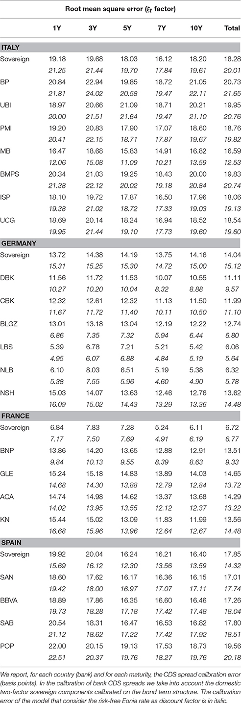
Table 3. Calibration error of the multi-factor Vasicek model.

The bank reporting the smallest calibration error is the German LBS with an overall RMSE equal to 6.06 (5.64 with the Eonia risk-free rates). The RMSE of this bank ranges from 5.21 bp for the 7-year maturity to 7.21 bp for the 5-year maturity, and, if one considers the spread with respect to the Eonia rate, it ranges from 4.84 bp for the 7-year maturity to 6.88 bp for the 5-year maturity. The bank reporting the largest calibration error is the Italian BP with an overall RMSE equal to 20.73 (21.65 with the Eonia risk-free rates). The RMSE of this bank ranges from 18.72 bp for the 7-year maturity to 22.94 bp for the 3-year maturity, and if one considers the spread with respect to the Eonia rate it ranges from 19.47 bp for the 7-year maturity to 24.02 bp for the 3-year maturity.

In order to compare the dynamics of estimated factors across banks, in Figure 5 we report the estimated dynamics of the bank specific factor ${\xi }_t^i$ (Eonia risk-free rates). They can be compared with the basis factor estimated in Section 5.2 and reported in Figure 4. The credit risk varies across banks. We recall that the total credit risk of each bank is given by the sovereign risk (δ_t) and the bank specific risk (${\xi }_t^i$). Therefore, the default intensity reported in Figure 5, has to be intended as the specific bank default intensity. We note that these dynamics varies across countries and banks, and they depend on the selected risk-free factor. Furthermore, in Tables 7, 8 we report the estimated parameters.

FIGURE 5

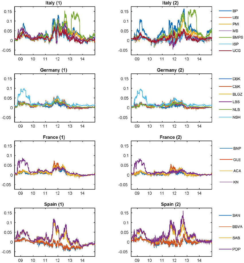
Figure 5. Default intensity processes based the multi-factor model with Vasicek dynamics for the 14 banks from June 30, 2008 to December 31, 2014. The Kalman filter is considered to extract the unobservable default intensity processes ξ_t (1) and γ_t (2). While in (1) we report the estimation of the factor driving the spread between bank CDS and the sovereign bond yield, in (2) we report the estimation of the factor driving the difference between bank and sovereign CDS quotes. We consider the risk-free rate Eonia as discount factor.

We note that the dynamics of this process may be partially affected by the fact that while the sovereign term structure ranges from 3-month (2-year for Spain) to 30-year, the bank CDS spread have only five maturities (1, 3, 5, 7, and 10 years).

In the second approach we assume that bank i default intensity has the following form

$x_t^{ban{k}_i}={\delta }_t+{\xi }_t^{so\upsilon }+{\gamma }_t^i,$

where δ_t represents the sovereign component calibrated on the sovereign bond term structure and ${\xi }_t^{soʋ}$ the component calibrated on the sovereign CDS-bond basis. Similarly to the first appraoch considered above, we divide the estimation exercise into different steps: (1) δ_t is estimated by considering the whole sovereign bond term structure over time (see Section 5.1); (2) the factor ${\xi }_t^{soʋ}$ is extracted by taking into consideration the estimate of δ_t together with the observed sovereign CDS spreads (see Section 5.2); (3) the specific factor for the bank i (i.e., ${\gamma }_t^i$) is extracted by taking into consideration the estimate of δ_t and ${\xi }_t^{soʋ}$ together with the observed bank i CDS spreads.

Figure 5 shows the dynamics of the estimated factors γ_t. As expected, due to the presence of a non zero sovereign CDS-bond basis, for each bank i the dynamics of ξ_t and γ_t are different. Furthermore, in Tables 9, 10 we report the estimated parameters and in Table 4 the corresponding calibration errors. The overall RMSE ranges from 6.12 bp to 23.97 bp (from 6.09 bp to 23.82 with the Eonia risk-free rates). As shown in Table 4, the calibration error depends on the maturity and on the bank.

TABLE 4

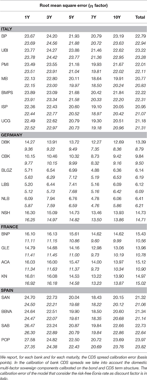
Table 4. Calibration error of the multi-factor Vasicek model.

TABLE 5

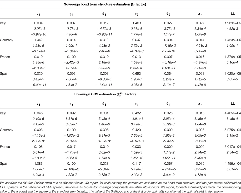
Table 5. Estimated parameters of the multi-factor Vasicek model.

TABLE 6

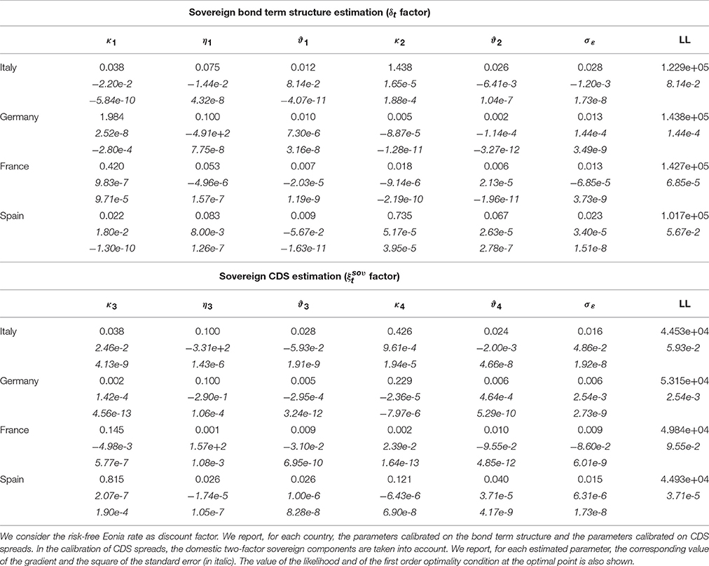
Table 6. Estimated parameters of the multi-factor Vasicek model.

TABLE 7

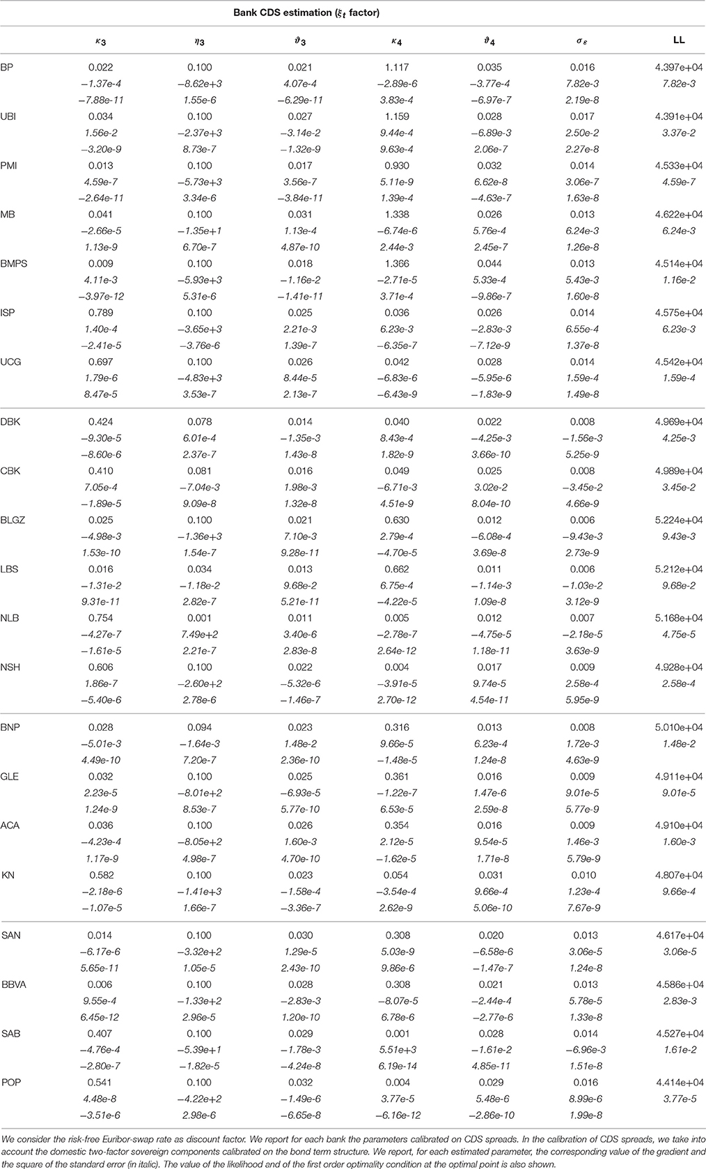
Table 7. Estimated parameters of the multi-factor Vasicek model.

TABLE 8

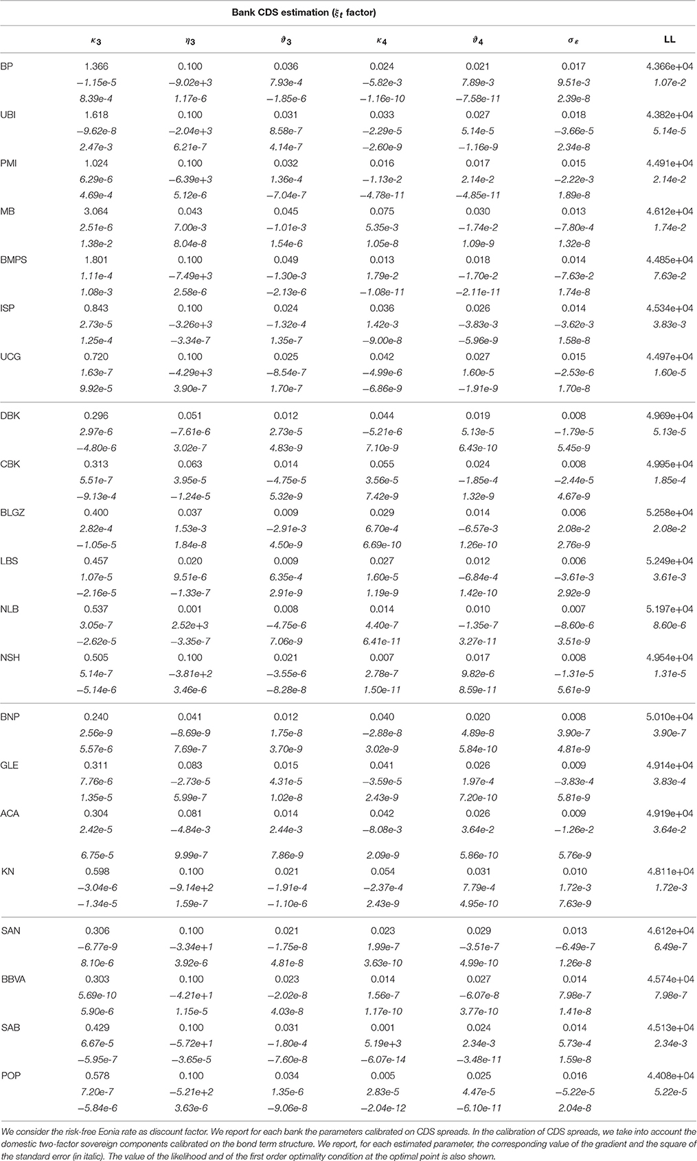
Table 8. Estimated parameters of the multi-factor Vasicek model.

TABLE 9

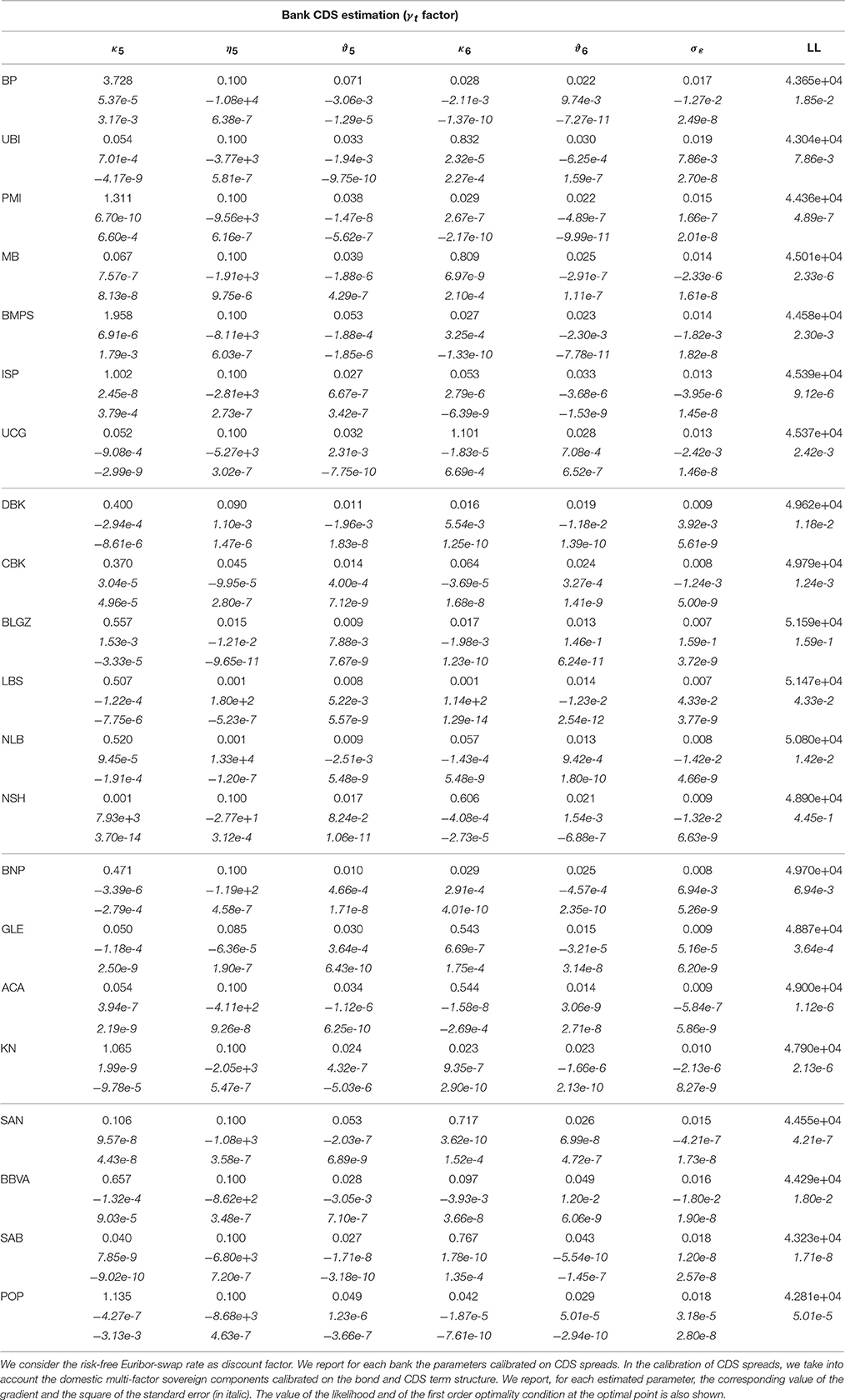
Table 9. Estimated parameters of the multi-factor Vasicek model.

TABLE 10

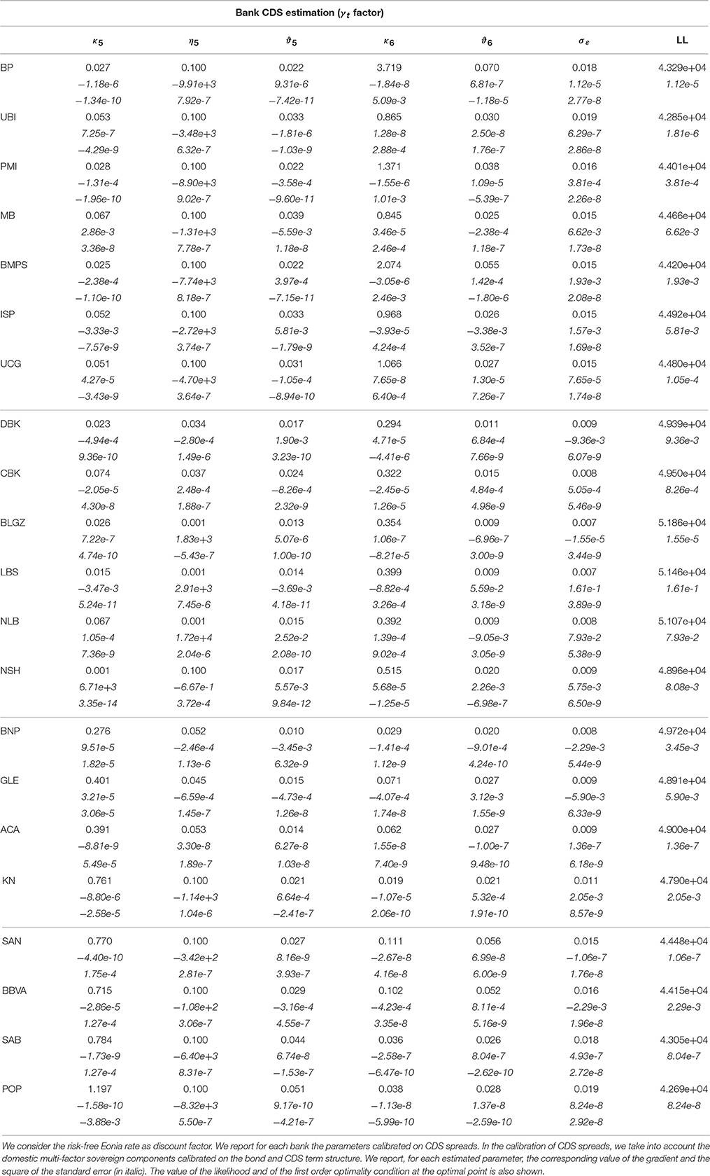
Table 10. Estimated parameters of the multi-factor Vasicek model.

There are no remarkable differences between the two calibration exercises (compare Tables 3, 4). In both calibration exercises, the specific bank risk is high for some banks over the observation period. Some banks report negative values for the factors ξ_t and γ_t, that is they are less risky than the sovereign. This is particularly evident for banks with large international activities based in Italy (UCG and ISP) and Spain (SAN and BBVA). In the last year (2014) for almost all banks, except BMPS and BP, the risk decreased. In the last 2 years the risk of German and French banks seems to be close to that of the sovereign. We point out that the behavior of ξ_t and γ_t is only a short-term indicator of the specific risk of the banks.

6. Conclusion

In this paper we implement a multi-factor model based on the standard Vasicek mean-reverting process to describe the dynamics of sovereign and bank CDS for different maturities by using the information content of risk-free rates and sovereign bonds term structure. We develop a unified framework in which sovereign bonds and sovereign and bank CDS quotes can be calibrated simultaneously (the approach could be also easily extended to the analysis of bonds issued by banks). The analysis is conducted by considering the dynamics of the driving factors under the risk-neutral measure, and it is repeated using either the Euribor-swap or the Eonia as discount factors.

For each country, we quantify the sovereign-specific credit risk factor by considering the sovereign bond term structure, while we explore the behavior of the sovereign CDS-bond basis by calibrating the spread between sovereign CDS quotes and bond yields. Then, we examine the dynamics of the short-term specific risk of banks, disentangling it from the sovereign risk factor that is common to all domestic banks in one country. We obtain this by following two different approaches: (1) the first one based on the sovereign bond yields only; (2) the second one based on both sovereign bond yields and sovereign CDS quotes. Note that while the estimated factors may give an idea on the short-term behavior of both credit and basis risk, the estimated parameter can be useful to capture the average slope and curvature of the term structure throughout the sample period. It is worth mentioning that, even if we assume that the dynamics of the risk factors are driven by Gaussian processes, the model calibration performance is satisfactory, although the calibration error varies across countries and banks.

From a practical perspective, disentangling the dynamics of a systemic risk factor and a bank-specific risk factor in the credit spread of banks debt instruments allows to timely monitor markets implicit assessment of the bank-sovereign nexus for selected institutions in each country. This is relevant from a micro-prudential perspective, as provides a more comprehensive measure of sovereign risk for individual banks than, for instance, direct exposures. At the same time, from a macro-prudential perspective, having a country-level instrinsic measure of the interconnectedness between sovereigns and their major domestic institutions allows to timely monitor one of the main risks to financial stability over recent years.

Future scenarios necessary for a proper assessment of different risks. Finally, even if we assume that the dynamics of the risk factors are driven by Gaussian processes, the model calibration performance is satisfactory. However, the calibration error varies across countries and banks.

Author Note

This publication should not be reported as representing the views of the Bank of Italy or of the European Central Bank (ECB). The views expressed are those of the authors and do not necessarily reflect those of the Bank of Italy or of the ECB.

Author Contributions

All authors listed, have made substantial, direct and intellectual contribution to the work, and approved it for publication.

Conflict of Interest Statement

The authors declare that the research was conducted in the absence of any commercial or financial relationships that could be construed as a potential conflict of interest.

Footnotes

1. ^Basel Committee for Banking Supervision, minimum capital requirements for market risk, January 2016.

2. ^If λ_t was a instantaneous short rate process, the same formula would represent the price at time 0 of a zero coupon bond maturing at t.

3. ^Here we assume a deterministic discount factor. Chen et al. [11, 14] considered a stochastic interest rate, and Dunbar [25] proposed a framework with stochastic factors to model interest rate and liquidity.

4. ^The calibrated spread for Germany, France and Spain are available upon request.

References

1. O'Donoghue B, Peacock M, Lee J, Capriotti L. A spread-return mean-reverting model for credit spread dynamics. Int J Theor Appl Finan. (2014) 17:1450017. doi: 10.1142/S0219024914500174

CrossRef Full Text | Google Scholar

2. Cont R. Credit default swaps and financial stability. Banque de France Finan Stab Rev. (2010) 35–43.

3. Brigo D, El-Bachir N. An exact formula for default swaptions pricing in the SSRJD stochastic intensity model. Math Finan. (2010) 20:365–82. doi: 10.1111/j.1467-9965.2010.00401.x

CrossRef Full Text | Google Scholar

4. Rebonato R, McKay K, White R. The SABR/LIBOR Market Model: Pricing, Calibration and Hedging for Complex Interest Rate Derivatives. Chichester: Wiley (2010).

Google Scholar

5. Brigo D, Mercurio F. Interest Rate Models: Theory and Practice: With Smile, Inflation, and Credit. Berlin; Heidelberg: Springer (2006).

Google Scholar

6. Grbac Z, Papapantoleon A. A tractable LIBOR model with default risk. Math Finan Econ. (2013) 7:203–27. doi: 10.1007/s11579-012-0090-5

CrossRef Full Text | Google Scholar

7. Nawalkha SK, Beliaeva NA, Soto G. A new taxonomy of the dynamic term structure models. J Invest Manage. (2010) 8.

Google Scholar

8. Cont R, Kan YH. Statistical modeling of credit default swap portfolios. In: Working Paper (2011).

9. Lucas A, Schwaab B, Zhang X. Conditional euro area sovereign default risk. J Business Econ Stat. (2014) 32:271–84. doi: 10.1080/07350015.2013.873540

CrossRef Full Text | Google Scholar

10. O'Kane D. The Link between Eurozone Sovereign Debt and CDS Prices. Technical Report, EDHEC-Risk Institute (2012).

Google Scholar

11. Chen RR, Cheng X, Fabozzi FJ, Liu B. An explicit, multi-factor credit default swap pricing model with correlated factors. J Finan Quantit Anal. (2008) 43:123–60. doi: 10.1017/S0022109000002775

CrossRef Full Text | Google Scholar

12. Jarrow RA, Li H, Ye X. Exploring statistical arbitrage opportunities in the term structure of CDS spreads. Working Paper (2009).

13. Carr P, Wu L. Stock options and credit default swaps: a joint framework for valuation and estimation. J Finan Econ. (2010) 8:409–49. doi: 10.1093/jjfinec/nbp010

CrossRef Full Text | Google Scholar

14. Chen RR, Cheng X, Wu L. Dynamic interactions between interest-rate and credit risk: theory and evidence on the credit default swap term structure. Rev Finan. (2013) 17:403–41. doi: 10.1093/rof/rfr032

CrossRef Full Text | Google Scholar

15. Ang A, Longstaff FA. Systemic sovereign credit risk: lessons from the US and Europe. J Monet Econ. (2013). 60:493–510. doi: 10.1016/j.jmoneco.2013.04.009

CrossRef Full Text | Google Scholar

16. Bianchi ML, Fabozzi FJ. Investigating the performance of non-Gaussian stochastic intensity models in the calibration of credit default swap spread. Comput Econ. (2015) 46:243–73. doi: 10.1007/s10614-014-9457-4

CrossRef Full Text | Google Scholar

17. Li J, Zinna G. On bank credit risk: systemic or bank-specific? Evidence from the US and the UK. In: Working Paper, Banca d'Italia n. 951 (2014a).

18. Li J, Zinna G. How much of bank credit risk is sovereign risk? Evidence from the Eurozone. In: Working Paper, Banca d'Italia n. 990 (2014b).

Google Scholar

19. Bianchi ML, Rocco M. Are Multi-factor Gaussian Term Structure Models Still Useful? An Empirical Analysis on Italian BTPs. (2015).

Google Scholar

20. Tassinari GL, Bianchi ML. Calibrating the smile with multivariate time-changed Brownian motion and the Esscher transform. Int J Theor Appl Finan. (2014) 17:1450023. doi: 10.1142/S021902491450023X

CrossRef Full Text | Google Scholar

21. Vasicek O. An equilibrium characterization of the term structure. J Finan Econ. (1977) 5:177–88. doi: 10.1016/0304-405X(77)90016-2

PubMed Abstract | CrossRef Full Text | Google Scholar

22. Jeanblanc M, Yor M, Chesney M. Mathematical Methods for Financial Markets. Berlin; Heidelberg: Springer (2009). doi: 10.1007/978-1-84628-737-4

CrossRef Full Text | Google Scholar

23. Duffie D, Filipović, D, Schachermayer W. Affine processes and applications in finance. Ann Appl Probabil. (2003) 13:984–1053. doi: 10.1214/aoap/1060202833

CrossRef Full Text | Google Scholar

24. O'Kane D, Turnbull S. Valuation of credit default swaps. Lehman Brothers, Fixed Income Quantitative Credit Research (2003).

25. Dunbar K. US corporate default swap valuation: the market liquidity hypothesis and autonomous credit risk. Quant Finan. (2008) 8:321–34. doi: 10.1080/14697680701397927

CrossRef Full Text | Google Scholar

26. Feldhütter P, Lando D. Decomposing swap spreads. J Finan Econ. (2008) 88:375–405. doi: 10.1016/j.jfineco.2007.07.004

CrossRef Full Text | Google Scholar

27. Ballotta L, Fusai G, Marazzina D. Integrated structural approach to Counterparty Credit Risk with dependent jumps, In: SSRN (2015).

28. Bianchetti M, Carlicchi M. Interest rates after the credit crunch - Multiple curve vanilla derivatives and SABR. Capco J Finan Transform Appl Finan. (2011). doi: 10.2139/ssrn.1905416

CrossRef Full Text | Google Scholar

29. Hull J, White A. Libor vs. OIS: the derivatives discounting dilemma. J Invest Manag. (2013) 11:14–27.

Google Scholar

30. Mayordomo S, Peña JI, Schwartz ES. Are all credit default swap databases equal? In: National Bureau of Economic Research, Working Paper No. 16590 (2010).

31. Amadei L, Di Rocco S, Gentile M, Grasso R, Siciliano G. Credit default swaps: contract characteristics and interrelations with the bond market. In: Consob, Discussion Papers (2011).

32. Pan J, Singleton KJ. Default and recovery implicit in the term structure of sovereign CDS spreads. J Finan. 63:2345–84 (2008). doi: 10.1111/j.1540-6261.2008.01399.x

CrossRef Full Text | Google Scholar

33. Lando D. Credit Risk Modeling: Theory and Applications. Princenton, NJ: Princeton University Press (2004).

Google Scholar

34. Haworth H, Schwarz C, Porter W. A tractable LIBOR model with default risk. Credit Suisse Fixed Income Res. (2009).

Google Scholar

35. Augustin P, Subrahmanyam MG, Tang DY, Wang SQ. Credit default swaps - A survey. Found Trends Finan. (2014) 9:1–196. doi: 10.1561/0500000040

CrossRef Full Text | Google Scholar