A study on the impact of household occupants’ behavior on energy consumption using an integrated computer model

Introduction

Occupants’ behaviors have a great impact on the building energy consumption as well as the peak loads typically experienced during the cooling season in summer time. Occupants could easily mitigate this by opening windows to use natural ventilation to reduce the cooling energy need in summer (Iwashita and Akasaka, 1997), and use a higher temperature setpoint in summer and a lower heating setpoint in winter for energy saving purposes (Newsham, 1997). Emery and Kippenhan (2006) observed that the energy need for heating the incoming cold air from the outside as a fraction of the total energy need in a house built in 1980 was approximately double that of an unoccupied house (29% compared with 14%). Paatero and Lund (2006) found that if the load of household appliances is shifted by 1 hr, the daily peak loads can be reduced by 7.2%, and with more severe demand site management schemes, the peak load at the yearly peak day can be reduced by 42%. Reinhart (2004) applied the probabilistic switching patterns (switching from electric lighting to daylighting) for a private office with a southern façade, and found that the lighting energy demand for a manually controlled electric lighting and shading system ranges from 10 to 39 kWh/(m² year). The predicted mean energy savings of a switch-off occupancy sensor in an office was 20% and the mean electric lighting energy savings due to a daylight-linked photocell control range was from 60% to 0. Bourgeois et al. (2006) found that for those occupants that actively seek daylighting rather than systematically rely on artificial lighting, the primary energy expenditure on lighting can be reduced by more than 40%, when compared with occupants who rely on constant artificial lighting. Al-Mumin et al. (2003) conducted a survey on occupancy patterns and operation schedules of electrical appliances in 30 houses in Kuwait. The computer simulation results showed an increase of 20% of the annual energy consumption compared with the results using default values of occupancy patterns from the program. Occupant behaviors are part of the building system, with implications on building energy use once changes in the behaviors are implemented (Lee and Malkawi, 2014). Several studies report that occupant behaviors significantly affect the energy demand of buildings (ranging from 1.0 to 2.84 times when comparing identical buildings) (Juodis et al., 2009; Maier et al., 2009). Therefore, it is very important to study the impact of occupants’ behaviors on the energy consumption of buildings and to identify what behaviors can be improved to reduce the building energy consumption.

From the literature survey above, the impact of the occupants’ behavior on the building energy consumption can be summarized as: (1) the occupants can open windows to allow natural ventilation for reduced cooling load in summer; (2) the occupants should use blinds to obstruct the solar radiation coming into the house to reduce the heat gain in summer and allow solar radiation to enter the house to reduce the heating energy need in winter; (3) occupants can vary the thermostat setpoint temperature to reduce cooling and heating energy demands in winter and summer seasons; and (4) the occupants’ should pay attention to the time of use of electrical appliances to avoid peak electricity demand time during the day.

Occupants’ living patterns were the first one to be investigated because it determines the existence of the occupants in the dwelling. They are either expressed as “diversity profile” (Papakostas and Sotiropoulos, 1997; Shimoda et al., 2007; Tanimoto et al., 2008) or a stochastic process (Page et al., 2008). In the “diversity profile” method, the occupants’ living patterns were generated from statistical data on averaged probabilities of respective activities at different characteristic days for different types of people. Living patterns are often applied in the simulation software. The stochastic model considers occupant presence as an inhomogeneous Markov chain interrupted by occasional periods of long absence and generates a time series of the state of presence (absent or present) of each occupant in a particular zone of the building. This approach is restrained by the time-step-size selection, which requires a transformation of the randomness from stochastic adaptive behaviors to building performance predictions (Gunay et al., 2013). Studies on window opening are mainly on field measurements on how long the window will be open/close (Jian et al., 2011) or the proportion of windows that were opened (Madhavi, 2010). Logistic regression models were developed to simulate the window open/close mechanism (Nicol and Humphreys, 2004; Rijal et al., 2007; Herkel et al., 2008; Andersen et al., 2009), but there is lack of literature on how wide the window will be opened to be integrated into building simulation software.

For multiple occupants’ behaviors, some researchers employed the framework approach (Lee and Malkawi, 2014; Hong et al., 2015). For example, Lee and Malkawi (2014) used an agent-based modeling approach to simulate five occupant behaviors in a commercial building including adjust clothing level, adjust activity level, window use, blind use, and space heater/personal fan use, Hong et al. (2015) presented a DNAs networks to model the energy-related occupant behavior in buildings.

Some building simulation programs, such as EnergyPlus¹ or ESP-r², offer the feasibility of programing to modify occupants’ behaviors by adding new occupancy models. However, the learning curve for both programs is very steep. Other programs, such as eQuest³ or Design Builder⁴ allow the user to modify the occupants’ living patterns. However, there is limitation on how much and to what extent a user can reprogram either one. In the meanwhile, the dynamic changes on how wide the window will be opened and the level of shading, as well as continuously adjusting thermostat setpoint are all very important factors that affect the thermal load and the final energy consumption of the buildings. The dynamic factors are difficult to be incorporated into building simulation software because they contradict with the current static settings. So, how to predict the impact of occupant behaviors on energy consumption in buildings more reliably?

To overcome limitations mentioned above, this paper introduces a holistic and integrated model (BMEOE), which considers the building enclosure, mechanical system, electrical appliances, occupants behavior, and external environment to simulate the building energy consumption. The model takes into account the proportion of the window opening (from fully close to fully open) and shading factor (from non-shading to fully shaded) as well as continuously adjusting thermostat setpoint, light-switching, and electrical appliances usage pattern. The results from the computer model are validated by simulation results from ESP-r, CFD modeling, and actual measurement obtained from the open literature. The model is then applied to a typical house located in the city of Oshawa (located 55 Km east of Toronto, ON, Canada), to examine the impact of occupants’ behavior on the energy consumption in residential buildings.

Mathematical Model

Heat Transfer through the Wall/Roof of the House

Governing Equation

The wall is assumed to have four layers, and there are two boundary nodes and one internal node for each layer, thus there are nine nodes for each wall/roof.

The governing equation for the transient heat transfer process is:

$\frac{\partial \text{T}}{\partial \text{t}}={\alpha }_{\text{h}}\frac{\partial {\text{T}}^2}{\partial {\text{x}}^2}$ (1)

Heat Balance Over the External Wall Surface

The heat balance over the external wall surface is written as follows:

$-k_1\frac{\partial \text{T}}{\partial \text{x}}|{}_{\text{x}=0}+q_{\text{sol,l,out}}+q_{\text{conv,l,out}}+q_{\text{surf,l,out}}={\rho }_1\cdot \frac{1}{4}{\text{dx}}_1\cdot c_{\text{p1}}\cdot \frac{\text{dT}}{\text{dt}}$ (2)

Internal Nodes Between Two Surfaces

For internal nodes between two different layers, the following equation is written, as an example for the surface between layers no.1 and 2:

$\begin{array}{c}\frac{1}{4}\cdot \left({\rho }_1\cdot c_{\text{p1}}\cdot {\text{dx}}_1+{\rho }_2\cdot c_{\text{p2}}\cdot {\text{dx}}_2\right)\cdot \frac{\text{dT}}{\text{dt}}=-k_1\cdot \frac{\text{dT}}{\text{dx}}|{}_{\text{x}=\frac{3}{4}{\text{dx}}_1}+k_2\cdot \frac{\text{dT}}{\text{dx}}|{}_{\text{x}={\text{dx}}_1+\frac{1}{4}{\text{dx}}_2}\end{array}$ (3)

Heat Balance Over the Inside Wall Surface

The heat balance over the inside wall surface is written as follows:

$\begin{array}{l}-k_4\cdot \frac{\partial \text{T}}{\partial \text{x}}|{}_{\text{x}=\text{th}}+q_{\text{sol,l,in}}+q_{\text{conv,l,in}}+q_{\text{surf,l,in}}+q_{\text{rad,ihg}}={\rho }_4\cdot \frac{1}{4}\cdot {\text{dx}}_4\cdot c_{\text{p4}}\cdot \frac{\text{dT}}{\text{dt}}\end{array}$ (4)

Window Model

As the window contains very little thermal mass, it is considered to behave in a quasi-steady state mode.

The heat transfer between two layers:

$q_{\text{win}}=U_{\text{w}}\left(T_{\text{os}}-T_{\text{is}}\right)$ (5)

where:

$U_{\text{w}}=\frac{1}{R_{\text{w}}}$ (6)

The heat transfer over the outer layer of the window:

$q_{\text{win}}=q_{\text{abs,sol,out}}+h_{\text{win,o}}\left(T_{\text{o}}-T_{\text{os}}\right)$ (7)

$q_{\text{win}}=q_{\text{abs,sol,in}}+q_{\text{igh,in}}+h_{\text{win,in}}\left(T_{\text{is}}-T_{\text{a}}\right)$ (8)

The optical properties of a double-pane window with each pane being standard 3.175 mm sheet glass have a set of polynomial coefficients as shown in Table 1. The transmittance and absorptance are calculated as follows (McQuiston et al., 2000):

${\tau }_{\text{Direct}}={\displaystyle \sum _{\text{j}=0}^5{t}_{\text{j}}{\text{cos}}^{\text{j}}\theta }$ (9)

${\tau }_{\text{diffuse}}={\displaystyle \sum _{\text{j}=0}^5\frac{t_{\text{j}}}{j+2}}$ (10)

${\alpha }_{\text{Direct,outer}}={\displaystyle \sum _{\text{j}=0}^5{a}_{\text{j,outer}}{\text{cos}}^{\text{j}}\theta }$ (11)

${\alpha }_{\text{diffuse,outer}}=2{\displaystyle \sum _{\text{j}=0}^5\frac{a_{\text{j,outer}}}{j+2}}$ (12)

${\alpha }_{\text{Direct,inner}}={\displaystyle \sum _{\text{j}=0}^5{a}_{\text{j,inner}}{\text{cos}}^{\text{j}}\theta }$ (13)

${\alpha }_{\text{diffuse,inner}}=2{\displaystyle \sum _{\text{j}=0}^5\frac{a_{\text{j,inner}}}{j+2}}$ (14)

TABLE 1

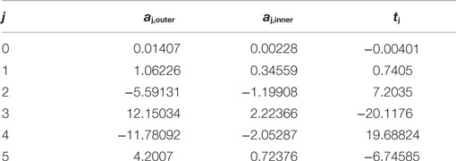
Table 1. Polynomial coefficients for a double-pane window with 3.175 mm sheet glass (Tanimoto et al., 2008).

The absorbed solar radiation over the outer layer of the window is calculated as:

$\begin{array}{c}{q}_{\text{sol,out}}=(1-\text{SF})({\alpha }_{\text{Direct,outer}}{G}_{\text{D}}+{\alpha }_{\text{diffuse,outer}}{G}_{\text{d}}+{\alpha }_{\text{diffuse,inner}}{q}_{\text{sol,in}})\end{array}$ (15)

The absorbed solar radiation over the inner layer of the window is calculated as:

$\begin{array}{c}{q}_{\text{sol,in}}=(1-\text{SF})({\alpha }_{\text{Direct,inner}}{G}_{\text{D}}+{\alpha }_{\text{diffuse,inner}}{G}_{\text{d}}+{\alpha }_{\text{diffuse,outer}}{q}_{\text{sol,in}})\end{array}$ (16)

Three double-glazed windows are considered, mounted on the south wall, east wall and west wall, respectively.

Air Flow Model

The air flow through the opening of the windows can be calculated by the crack method (ASHRAE, 1992):

$\stackrel{\text{.}}{m}=C_{\text{d}}\cdot \rho \cdot A\cdot {(\text{Δ}p)}^{\text{n}}$ (17)

$\text{Δ}p=\text{Δ}{p}_{\text{w}}+\text{Δ}{p}_{\text{s}}+\text{Δ}{p}_{\text{p}}$ (18)

$\text{Δ}{p}_{\text{w,i}}=\frac{1}{2}\left(C_{\text{p,i}}-C_{\text{p,a}}\right){\rho }_{\text{o}}{v}_{\text{w}}^2$ (19)

The pressure difference due to stack effect can be calculated as (McQuiston et al., 2000):

$\begin{array}{c}\text{Δ}{p}_{\text{s}}=\frac{C_{\text{f}}}{R_{\text{a}}}\cdot p_{\text{o}}\cdot \left(\frac{1}{T_{\text{o}}}-\frac{1}{T_{\text{a}}}\right)\cdot \left(\frac{H}{2}-h\right)\approx 0\text{.0342}\cdot p_{\text{o}}\cdot \left(\frac{1}{T_{\text{o}}}-\frac{1}{T_{\text{a}}}\right)\cdot \left(\frac{H}{2}-h\right)\end{array}$ (20)

where $\frac{H}{2}-h$ is the distance to the neutral plane, assumed at mid-height of the window (m).

Air flow can occur through one opening or more than one opening (e.g., two openings or three openings) as a combination of stack effect and wind pressure.

For single opening or more than one opening without wind pressure:

$\begin{array}{l}d\text{(}\stackrel{\text{.}}{m\text{)}}=C_{\text{d}}\cdot \rho \cdot {\left(\text{Δ}{p}_{\text{s}}\right)}^{\text{n}}\text{dA}\\ =C_{\text{d}}\cdot \rho \cdot {\left(0\text{.0342}\cdot p_{\text{o}}\cdot \left(\frac{1}{T_{\text{o}}}-\frac{1}{T_{\text{a}}}\right)\cdot \left(\frac{H}{2}-h\right)\right)}^{\text{n}}\cdot \text{OF}\cdot W\text{dh}\end{array}$ (21)

Therefore,

$\begin{array}{l}\stackrel{\text{.}}{m}={\displaystyle \underset{0}{\overset{\frac{\text{H}}{2}}{\int }}{C}_{\text{d}}\cdot \rho \cdot {\left(0\text{.0342}\cdot p_{\text{o}}\cdot \left(\frac{1}{T_{\text{o}}}-\frac{1}{T_{\text{a}}}\right)\cdot \left(\frac{H}{2}-h\right)\right)}^{\text{n}}\cdot \text{OF}\cdot W}\text{dh}\\ =C_{\text{d}}\cdot \rho \cdot \text{OF}\cdot W\cdot {\left(0\text{.0342}\cdot p_{\text{o}}\cdot \left|\left(\frac{1}{T_{\text{o}}}-\frac{1}{T_{\text{a}}}\right)\right|\right)}^{\text{n}}{\left(\frac{H}{2}\right)}^{\text{n}+1}\left(\frac{1}{n+1}\right)\end{array}$ (22)

For more than one opening with stack effect and wind-driven ventilation, a mass balance approach is applied:

${\displaystyle \sum _{\text{i}=1}^{\text{N}}\stackrel{\text{.}}{m_{\text{i}}}}=0$ (23)

The combination of the stack effect and the wind pressure results in the shift of the neutral plane (Figure 1). It can be divided into three types: (1) H_N ≥ H; (2) 0 < H_N < H; (3) H_N ≤ 0. The position of the new neutral plane for each window can be calculated by:

$\text{Δ}{p}_{\text{w}}+\text{Δ}{p}_{\text{s}}=0$ (24)

FIGURE 1

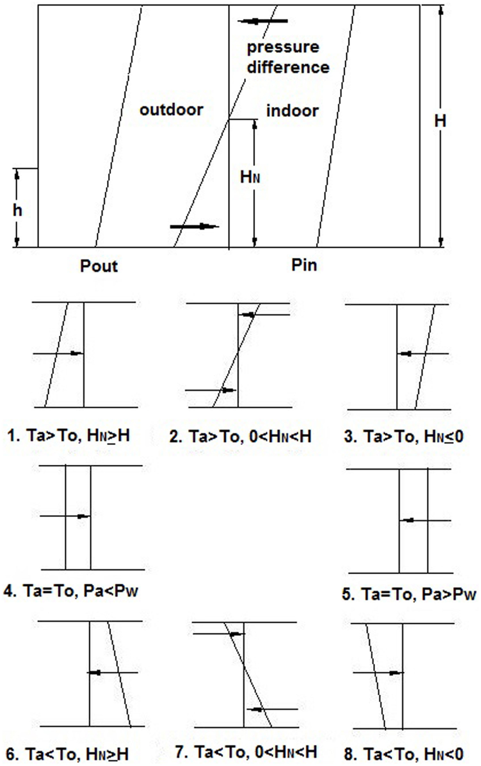
Figure 1. Air flow through the window due to stack effect and wind pressure.

Substituting Eqs 19 and 20 into Eq. 24, and the following equation can be derived:

$\begin{array}{l}\frac{1}{2}\text{(}{C}_{\text{p,i}}-C_{\text{p,a}}\text{)}{\rho }_{\text{o}}{v}_{\text{w}}^2+0\text{.0342}\cdot p_{\text{o}}\cdot \left(\frac{1}{T_{\text{o}}}-\frac{1}{T_{\text{a}}}\right)\cdot \left(\frac{H}{2}-H_{\text{N}}\right)=0\end{array}$ (25)

Therefore,

$H_{\text{N}}=\frac{\frac{1}{2}\text{(}{C}_{\text{p,i}}-C_{\text{p,a}}\text{)}{\rho }_{\text{o}}{v}_{\text{w}}^2}{0\text{.0342}\cdot p_{\text{o}}\cdot \left(\frac{1}{T_{\text{o}}}-\frac{1}{T_{\text{a}}}\right)}+\frac{H}{2}$ (26)

The air flow through one opening of the window for type no.1 is calculated as:

$\begin{array}{l}\stackrel{\text{.}}{\begin{array}{l}\stackrel{\text{.}}{m_{\text{i}}}={\displaystyle \underset{0}{\overset{\text{H}}{\int }}{C}_{\text{d}}\cdot \rho \cdot \text{OF}\cdot W}\times {\left(\text{(}{C}_{\text{p,i}}-C_{\text{p,a}}\text{)}{p}_{\text{w}}+0\text{.0342}\cdot p_{\text{o}}\cdot \left(\frac{1}{T_{\text{o}}}-\frac{1}{T_{\text{a}}}\right)\cdot \left(\frac{H}{2}-h\right)\right)}^{\text{n}}\text{dh}\end{array}}\\ =\frac{C_{\text{d}}\cdot \rho \cdot \text{OF}\cdot W}{\text{(}n+\text{1)}\cdot 0\text{.0342}\cdot p_{\text{o}}\cdot \left(\frac{1}{T_{\text{o}}}-\frac{1}{T_{\text{a}}}\right)}\times \left(\begin{array}{l}{\left(\text{(}{C}_{\text{p,i}}-C_{\text{p,a}}\text{)}{p}_{\text{w}}+0\text{.0342}\cdot p_{\text{o}}\cdot \left(\frac{1}{T_{\text{o}}}-\frac{1}{T_{\text{a}}}\right)\cdot \left(\frac{H}{2}\right)\right)}^{\text{n}+1}-\\ {\left(\text{(}{C}_{\text{p,i}}-C_{\text{p,a}}\text{)}{p}_{\text{w}}+0\text{.0342}\cdot p_{\text{o}}\cdot \left(\frac{1}{T_{\text{o}}}-\frac{1}{T_{\text{a}}}\right)\cdot \left(-\frac{H}{2}\right)\right)}^{\text{n}+1}\end{array}\right)\end{array}$ (27)

The air flow through one opening of the window for type no. 2 is calculated as:

$\begin{array}{l}\stackrel{\text{.}}{\begin{array}{l}\stackrel{\text{.}}{m_{\text{i}}}={\displaystyle \underset{0}{\overset{{\text{H}}_{\text{N}}}{\int }}{C}_{\text{d}}\cdot \rho \cdot \text{OF}\cdot W}\times {\left(\text{(}{C}_{\text{p,i}}-C_{\text{p,a}}\text{)}{p}_{\text{w}}+0\text{.0342}\cdot p_{\text{o}}\cdot \left(\frac{1}{T_{\text{o}}}-\frac{1}{T_{\text{a}}}\right)\cdot \left(\frac{H}{2}-h\right)\right)}^{\text{n}}\text{dh}-\end{array}}\\ \begin{array}{cc}& \end{array}{\displaystyle \underset{{\text{H}}_{\text{N}}}{\overset{\text{H}}{\int }}{C}_{\text{d}}\cdot \rho \cdot \text{OF}\cdot W}\times {\left(-\text{(}{C}_{\text{p,i}}-C_{\text{p,a}}\text{)}{p}_{\text{w}}-0\text{.0342}\cdot p_{\text{o}}\cdot \left(\frac{1}{T_{\text{o}}}-\frac{1}{T_{\text{a}}}\right)\cdot \left(\frac{H}{2}-h\right)\right)}^{\text{n}}\text{dh}\\ =\frac{C_{\text{d}}\cdot \rho \cdot \text{OF}\cdot \text{W}}{\text{(}n+\text{1)}\cdot 0\text{.0342}\cdot p_{\text{o}}\cdot \left(\frac{1}{T_{\text{o}}}-\frac{1}{T_{\text{a}}}\right)}\times \left(\begin{array}{l}{\left(\text{(}{C}_{\text{p,i}}-C_{\text{p,a}}\text{)}{p}_{\text{w}}+0\text{.0342}\cdot p_{\text{o}}\cdot \left(\frac{1}{T_{\text{o}}}-\frac{1}{T_{\text{a}}}\right)\cdot \left(\frac{H}{2}\right)\right)}^{\text{n}+1}-\\ {\left(-\text{(}{C}_{\text{p,i}}-C_{\text{p,a}}\text{)}{p}_{\text{w}}-0\text{.0342}\cdot p_{\text{o}}\cdot \left(\frac{1}{T_{\text{o}}}-\frac{1}{T_{\text{a}}}\right)\cdot \left(-\frac{H}{2}\right)\right)}^{\text{n}+1}\end{array}\right)\end{array}$ (28)

The air flow through one opening of the window for type no. 3 is calculated from:

$\begin{array}{l}\stackrel{\text{.}}{m_{\text{i}}}={\displaystyle \underset{0}{\overset{\text{H}}{\int }}{C}_{\text{d}}\cdot \rho \cdot \text{OF}\cdot W}{\left(-\text{(}{C}_{\text{p,i}}-C_{\text{p,a}}\text{)}{p}_{\text{w}}-0\text{.0342}\cdot p_{\text{o}}\cdot \left(\frac{1}{T_{\text{o}}}-\frac{1}{T_{\text{a}}}\right)\cdot \left(\frac{H}{2}-h\right)\right)}^{\text{n}}\text{dh}\\ =-\frac{C_{\text{d}}\cdot \rho \cdot \text{OF}\cdot W}{\text{(}n+\text{1)}\cdot 0\text{.0342}\cdot p_{\text{o}}\cdot \left(\frac{1}{T_{\text{o}}}-\frac{1}{T_{\text{a}}}\right)}\left(\begin{array}{l}{\left(-\text{(}{C}_{\text{p,i}}-C_{\text{p,a}}\text{)}{p}_{\text{w}}-0\text{.0342}\cdot p_{\text{o}}\cdot \left(\frac{1}{T_{\text{o}}}-\frac{1}{T_{\text{a}}}\right)\cdot \left(-\frac{H}{2}\right)\right)}^{\text{n}+1}-\\ {\left(-\text{(}{C}_{\text{p,i}}-C_{\text{p,a}}\text{)}{p}_{\text{w}}-0\text{.0342}\cdot p_{\text{o}}\cdot \left(\frac{1}{T_{\text{o}}}-\frac{1}{T_{\text{a}}}\right)\cdot \left(\frac{H}{2}\right)\right)}^{\text{n}+1}\end{array}\right)\end{array}$ (29)

If T_o = T_a, there will be no stack effect.

If C_p,i < C_p,a (type no. 4):

$\stackrel{\text{.}}{m_{\text{i}}}=-C_{\text{d}}\cdot \rho \cdot \text{OF}\cdot W\cdot H\cdot {\left(-\text{(}{C}_{\text{p,i}}-C_{\text{p,a}}\text{)}{p}_{\text{w}}\right)}^{\text{n}}$ (30)

If C_p,i ≥ C_p,a (type no. 5):

$\stackrel{\text{.}}{m_{\text{i}}}=C_{\text{d}}\cdot \rho \cdot \text{OF}\cdot \text{W}\cdot H\cdot {\left(\text{(}{C}_{\text{p,i}}-C_{\text{p,a}}\text{)}{p}_{\text{w}}\right)}^{\text{n}}$ (31)

If T_o < T_a, there will be three cases exist: (1) H_N ≥ H; (2) 0 < H_N < H; (3) H_N ≤ 0.

For H_N ≥ H (type no. 6):

$\begin{array}{l}{\dot{m}}_i=-{\displaystyle \underset{0}{\overset{\text{H}}{\int }}{C}_{\text{d}}\cdot \rho \cdot \text{OF}\cdot W}\times {\left(-\text{(}{C}_{\text{p,i}}-C_{\text{p,a}}\text{)}{p}_{\text{w}}-0\text{.0342}\cdot p_{\text{o}}\cdot \left(\frac{1}{T_{\text{o}}}-\frac{1}{T_{\text{a}}}\right)\cdot \left(\frac{H}{2}-h\right)\right)}^{\text{n}}\text{dh}\\ \begin{array}{cc}& =\end{array}-\frac{C_{\text{d}}\cdot \rho \cdot \text{OF}\cdot W}{\text{(}n+\text{1)}\cdot 0\text{.0342}\cdot p_{\text{o}}\cdot \left(\frac{1}{T_{\text{o}}}-\frac{1}{T_{\text{a}}}\right)}\times \left(\begin{array}{l}{\left(-\text{(}{C}_{\text{p,i}}-C_{\text{p,a}}\text{)}{p}_{\text{w}}-0\text{.0342}\cdot p_{\text{o}}\cdot \left(\frac{1}{T_{\text{o}}}-\frac{1}{T_{\text{a}}}\right)\cdot \left(-\frac{H}{2}\right)\right)}^{\text{n}+1}\\ -{\left(-\text{(}{C}_{\text{p,i}}-C_{\text{p,a}}\text{)}{p}_{\text{w}}-0\text{.0342}\cdot p_{\text{o}}\cdot \left(\frac{1}{T_{\text{o}}}-\frac{1}{T_{\text{a}}}\right)\cdot \left(\frac{H}{2}\right)\right)}^{\text{n}+1}\end{array}\right)\end{array}$ (32)

For 0 < H_N < H(type no. 7):

$\begin{array}{l}\stackrel{\text{.}}{m_{\text{i}}}=-{\displaystyle \underset{0}{\overset{{\text{H}}_{\text{N}}}{\int }}{C}_{\text{d}}\cdot \rho \cdot \text{OF}\cdot W}\times {\left(-\text{(}{C}_{\text{p,i}}-C_{\text{p,a}}\text{)}{p}_{\text{w}}-0\text{.0342}\cdot p_{\text{o}}\cdot \left(\frac{1}{T_{\text{o}}}-\frac{1}{T_{\text{a}}}\right)\cdot \left(\frac{H}{2}-h\right)\right)}^{\text{n}}\text{dh}\\ +{\displaystyle \underset{{\text{H}}_{\text{N}}}{\overset{\text{H}}{\int }}{C}_{\text{d}}\cdot \rho \cdot \text{OF}\cdot W}\times {\left(\text{(}{C}_{\text{p,i}}-C_{\text{p,a}}\text{)}{p}_{\text{w}}+0\text{.0342}\cdot p_{\text{o}}\cdot \left(\frac{1}{T_{\text{o}}}-\frac{1}{T_{\text{a}}}\right)\cdot \left(\frac{H}{2}-h\right)\right)}^{\text{n}}\text{dh}\\ =-\frac{C_{\text{d}}\cdot \rho \cdot \text{OF}\cdot W}{\text{(}n+\text{1)}\cdot 0\text{.0342}\cdot p_{\text{o}}\cdot \left(\frac{1}{T_{\text{o}}}-\frac{1}{T_{\text{a}}}\right)}\times \left(\begin{array}{l}{\left(-\text{(}{C}_{\text{p,i}}-C_{\text{p,a}}\text{)}{p}_{\text{w}}-0\text{.0342}\cdot p_{\text{o}}\cdot \left(\frac{1}{T_{\text{o}}}-\frac{1}{T_{\text{a}}}\right)\cdot \left(\frac{H}{2}\right)\right)}^{\text{n}+1}\\ -{\left(\text{(}{C}_{\text{p,i}}-C_{\text{p,a}}\text{)}{p}_{\text{w}}+0\text{.0342}\cdot p_{\text{o}}\cdot \left(\frac{1}{T_{\text{o}}}-\frac{1}{T_{\text{a}}}\right)\cdot \left(-\frac{H}{2}\right)\right)}^{\text{n}+1}\end{array}\right)\end{array}$ (33)

For H_N ≤ 0 (type no. 8):

$\begin{array}{l}\stackrel{\text{.}}{m_{\text{i}}}={\displaystyle \underset{0}{\overset{\text{H}}{\int }}{C}_{\text{d}}\cdot \rho \cdot \text{OF}\cdot W}\times {\left(\text{(}{C}_{\text{p,i}}-C_{\text{p,a}}\text{)}{p}_{\text{w}}+0\text{.0342}\cdot p_{\text{o}}\cdot \left(\frac{1}{T_{\text{o}}}-\frac{1}{T_{\text{a}}}\right)\cdot \left(\frac{H}{2}-h\right)\right)}^{\text{n}}\text{dh}\\ \begin{array}{cc}& =\end{array}-\frac{C_{\text{d}}\cdot \rho \cdot \text{OF}\cdot W}{\text{(}n+\text{1)}\cdot 0\text{.0342}\cdot p_{\text{o}}\cdot \left(\frac{1}{T_{\text{o}}}-\frac{1}{T_{\text{a}}}\right)}\times \left(\begin{array}{l}{\left(\text{(}{C}_{\text{p,i}}-C_{\text{p,a}}\text{)}{p}_{\text{w}}+0\text{.0342}\cdot p_{\text{o}}\cdot \left(\frac{1}{T_{\text{o}}}-\frac{1}{T_{\text{a}}}\right)\cdot \left(-\frac{H}{2}\right)\right)}^{\text{n}+1}\\ -{\left(\text{(}{C}_{\text{p,i}}-C_{\text{p,a}}\text{)}{p}_{\text{w}}+0\text{.0342}\cdot p_{\text{o}}\cdot \left(\frac{1}{T_{\text{o}}}-\frac{1}{T_{\text{a}}}\right)\cdot \left(\frac{H}{2}\right)\right)}^{\text{n}+1}\end{array}\right)\end{array}$ (34)

Electrical Appliances Power Input Model

The operating electric energy consumption for the electric appliances working on multi-stage operating conditions is:

$E_{\text{i}}=f_{\text{h},\text{i}}{}^{\star }{\text{AVG}}_{\text{i}}$ (35)

${\text{AVG}}_{\text{i}}=\frac{{\displaystyle \sum _{\text{j}=1}^{\text{N}}{P}_{\text{i,j}}{\tau }_{\text{j}}}}{{\displaystyle \sum _{\text{j}=1}^{\text{N}}{\tau }_{\text{j}}}}$ (36)

If it is a group of appliances:

${\text{AVG}}_{\text{i}}=\frac{{\displaystyle \sum _{\text{k}=1}^{\text{M}}{f}_{\text{d,k}}}\frac{{\displaystyle \sum _{\text{j}=1}^{\text{N}}{P}_{\text{k,j}}{\tau }_{\text{j}}}}{{\displaystyle \sum _{\text{j}=1}^{\text{N}}{\tau }_{\text{j}}}}}{{\displaystyle \sum _{\text{k}=1}^{\text{M}}{f}_{\text{d,k}}}}$ (37)

The electric appliances include freezer, refrigerator, lighting, clothes washer, dish washer, TV, second TV, oven, etc.

Heat Balance of the Inside Air

The indoor air of the house is assumed well mixed and therefore it is represented by one node. The indoor air temperature T_a is held at the thermostat setpoint value by a heating/cooling system. The heat balance for the indoor air is written as:

$Q_{\text{HVAC}}+{\displaystyle \sum _{\text{j}=1}^{\text{M}}{A}_{\text{j}}}{h}_{\text{a}}\left(T_{\text{j,in}}-T_{\text{a}}\right)+Q_{\text{inf}}+Q_{\text{internal,conv}}=0$ (38)

House Energy Consumption

In this system, the house is heated by forced air and cooled by a central air conditioning unit, and the same duct systems are used for heating and cooling (Figure 2). The following are the components of the whole system: (1) Heating: forced air heating system with heat supplied by a gas-fired furnace; (2) DHW: gas-fired hot water tank; (3) Ventilation: exhaust fan; and (4) Cooling: central air conditioning unit.

FIGURE 2

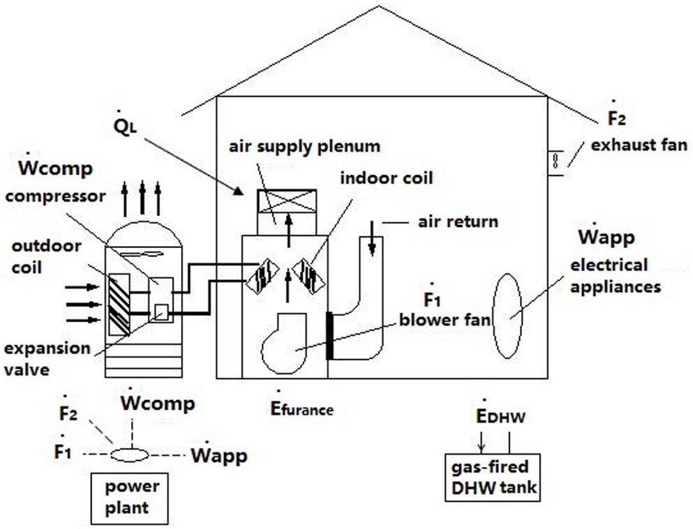
Figure 2. A typical house in Oshawa.

The following conditions applied:

$Q_{\text{ac}}=-Q_{\text{HVAC}}(\text{summer season})$ (39)

$Q_{\text{furnance}}=Q_{\text{HVAC}}\left(\text{winter season}\right)$ (40)

Total electricity demand is:

$W_{\text{pp}}=W_{\text{blower}}+W_{\text{exhaust}}+W_{\text{comp}}+W_{\text{app}}$ (41)

Total energy need of the house is:

$E_{\text{total}}=E_{\text{pp}}+E_{\text{furnace}}+E_{\text{DHW}}$ (42)

Figure 3 presents an overview of the relationships among the models. The heat transfer through the wall/roof model calculates the temperature profiles of the wall/roof/floor and pass the inside surface temperature to the heat balance model; the window model calculates the temperature profiles of the window and pass the inside window surface temperature to the heat balance of the inside air model; the air flow model calculates the infiltration/exfiltration rate and pass it to the heat balance of the inside air model; the electrical appliances power input model calculates the appliances electrical demand and pass it to the house energy consumption, and at the same time calculates the convective internal heat gain of the electrical appliances and pass it to the heat balance of the inside air model; the heat balance of the inside air model calculates the heating and cooling load and pass it to the house energy consumption model; the purpose of the house energy consumption calculates the final house energy consumption.

FIGURE 3

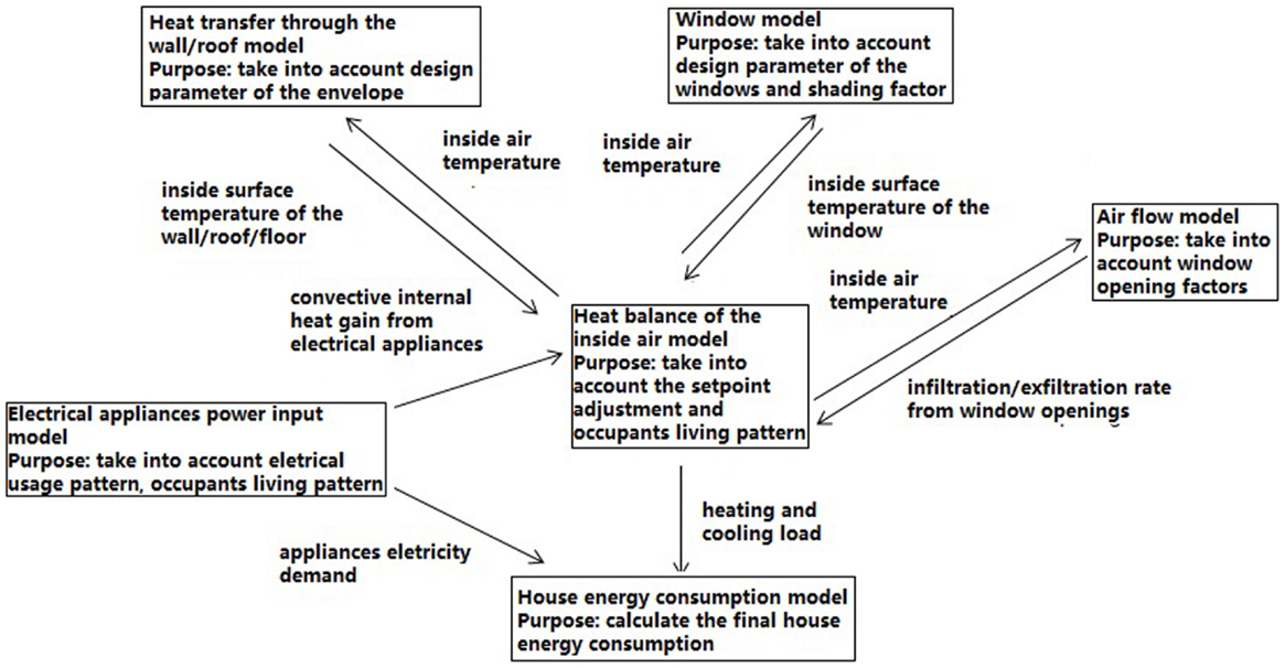
Figure 3. Overview of the relationships among the models.

Numerical Solution

The thermal and airflow model is written as a system of linear and non-linear equations. Non-linear equations are generated due to the surface-to-surface long-wave radiation in the thermal model, and also due to the coupling of air movement and heat transfer between the house and outdoor environment. However, if the radiation coefficients are used to calculate the surface-to-surface radiation, then the whole system of equations for temperatures can be considered as quasi-linear. The radiation coefficients are generated by using the total interchange view factor (Lin and Zmeureanu, 2008). The system of equations can then be broken into two sub-systems; one system that contains the unknown temperatures and another system that contains the unknown pressure coefficients.

The convective heat-transfer coefficients are calculated based on the updated air temperature difference, air flow direction and air velocity. The radiation coefficients are calculated using the total interchange view factor and the updated surface temperature difference.

The system of equations of the thermal and airflow models are written in form of a matrix:

$\left[\begin{array}{cc}A& O\\ O& C\end{array}\right]\left[\begin{array}{c}T\\ {\mathbf{C}}_{\mathbf{P}}\end{array}\right]=\left[\begin{array}{c}B\\ D\end{array}\right]$ (43)

where A is the matrix containing the thermal and optical properties of the system; C is the matrix containing the properties of the interfaces between the indoor and outdoor; B and D contain the coefficients of the driving forces for temperature and pressure, respectively.

By using the radiation coefficient and convective heat transfer coefficient through iteration (Lin and Zmeureanu, 2008), the entire system of equations is written separately as composed of a linearized part that contains the unknown temperatures only:

$\left[A\right]\begin{array}{c}\end{array}\left[T\right]=\left[B\right],$ (44)

and a non-linearized part that contains the unknown pressures only:

$\left[\mathbf{C}\right]\begin{array}{c}\end{array}\left[{\mathbf{C}}_{\mathbf{P}}\right]=\left[D\right].$ (45)

For a house with three double-glazed windows, the total number of unknown temperatures of the system Eq. 44 is 60.

The linearized part of the system (equations for temperature) is solved by the Gauss-Seidel iteration technique, and the non-linear part of the system (equations for pressure) is solved by the Newton-Raphson method (Press et al., 1992).

Validation

The simulation results of the thermal load of a house located in Oshawa were compared with the results from the ESP-r program (Figure 4). The house dimensions are 10 m × 10 m × 4 m, and includes three double-glazed windows which are mounted on the south wall, west wall and east wall, respectively. The window-to-wall ratio of 0.15 is applied. Thermal resistance of the external walls is 3.4 m² K/W, and of the roof is 5.5 m² K/W. The U-value of the windows is 3.06 W/m² K. The natural air infiltration rate for the house is set equal to 0.15 ACH, and the thermostat setpoint temperature is 22.5°C. No internal heat gain is considered. The simulation results from the computer program predicted the annual energy needs of 30,733 kWh, while the simulation results from the ESP-r program predicted the annual energy needs of 29,766 kWh. The difference between the results from the computer program and that of the ESP-r program was only 3.2%. The simulation results are in good agreement with the results from the ESP-r program.

FIGURE 4

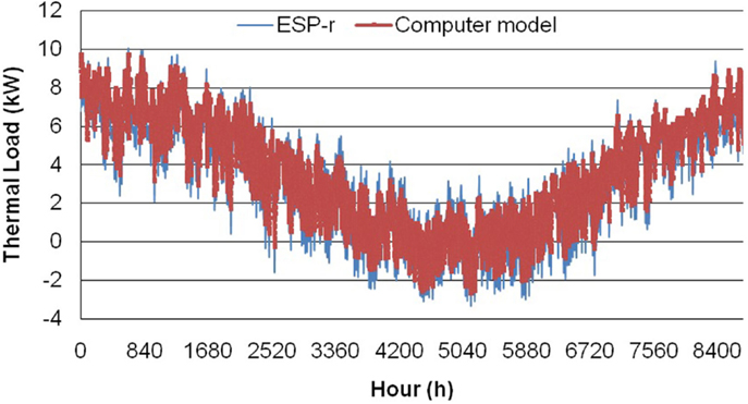
Figure 4. Predictions of the hourly thermal load, comparisons between Computer model and ESP-r program.

The results of the ventilation model (which was used to calculate the air flow through the window openings) were compared with the results from the CFD studies of (Asfour and Gadi, 2007) for windows with two openings at opposite site. The wind speed was 1.0 m/s, and wind direction was either normal to the window (cases No.1 and 3), or oblique to the window (case No. 2). Detailed information of the three cases are presented in Table 2. The simulation results presented in Table 3 indicate that the ventilation results are also in good agreement with the CFD results, with a difference of less than 5%.

TABLE 2

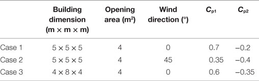
Table 2. Information for the cases tested in this study.

TABLE 3

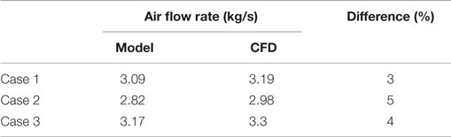
Table 3. Simulation results vs. CFD results.

The results from the power input model for the electric appliances were compared with the mean hourly consumption curve of a household during weekends provided by Paatero and Lund (2006). The results are presented in Figure 5, and it is observed that the average difference between the power plant model and the mean hourly household electricity consumption is about 6.5%.

FIGURE 5

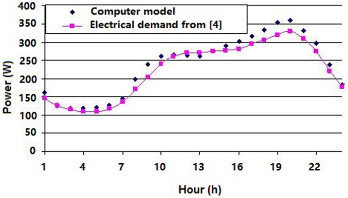
Figure 5. Comparison of the hourly household appliances electricity demand.

The results of the energy consumption are compared with measurement data on a house in Oshawa which was audited. Thermal resistance of the external walls and roof is 3.3 m² K/W. The U-value of the windows is 2.5 W/m² K. The natural air infiltration rate for the house is set equal to 0.075 ACH, heating and cooling by a central air-conditioning system. The results are presented in Figure 6. The computer model predicted total energy consumption of 23,389 kWh while the measurement result was 21,539 kWh. The average difference between the result from the computer model and measurement is about 6.6%.

FIGURE 6

Figure 6. Comparison on the energy consumption, computer simulation vs. measurement data.

Overall, the predictions of the ventilation model and electricity power input model, as well as the energy consumption, are comparable with those obtained from a detailed CFD model and with the experimental measurement.

Case Studies

A house of 100 m² floor area and 4 m wall height, located in Oshawa, ON, Canada, is selected as a case study. Table 4 presents a list of the inputs parameters for the computer model, where occupants living pattern and opening factor of the window represent window opening behaviors; occupants living pattern and shading factor of the window represent window shading behaviors; occupants living pattern and light switching pattern represent light switching behaviors; occupants living pattern and thermostat setpoint represent thermostat adjusting behavior; electrical appliances using habit represent electrical appliances using behaviors. The outdoor dry bulb temperature, humidity ratio, direct normal solar radiation, global solar radiation, diffuse solar radiation, wind speed, and wind direction were obtained from EnergyPlus⁵ weather file database. The average dry bulb temperature and direct normal solar radiation are presented in Figures 7 and 8. Each wall of the house is composed of 100 mm face brick, 135 mm insulation, and 20 mm gypsum board. The window-to-wall ratio of 15% is applied to three facades only (East, South, and West). The natural air infiltration rate for the house is set equal to 0.15 ach for newly built house, and 0.5 for old house. The house has one stove oven, one clothes washer, one dish washer, one freezer, and one color TV. The living patterns come from studies by (Papakostas and Sotiropoulos, 1997; Al-Mumin et al., 2003). The occupants’ living patterns and electric appliances usage are summarized in Table 5.

TABLE 4

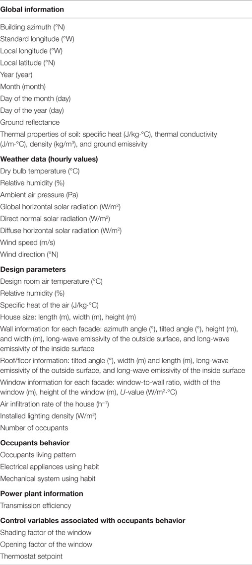
Table 4. Input parameters for the computer model.

FIGURE 7

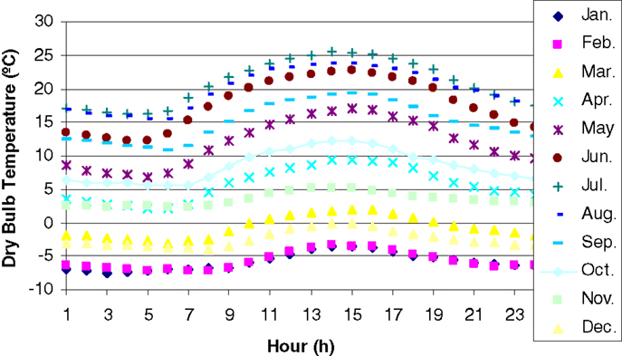
Figure 7. Ambient air temperature for case study.

FIGURE 8

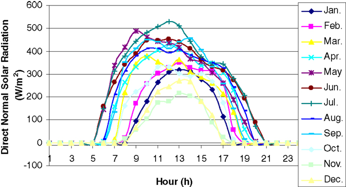
Figure 8. Direct normal solar radiation for case study.

TABLE 5

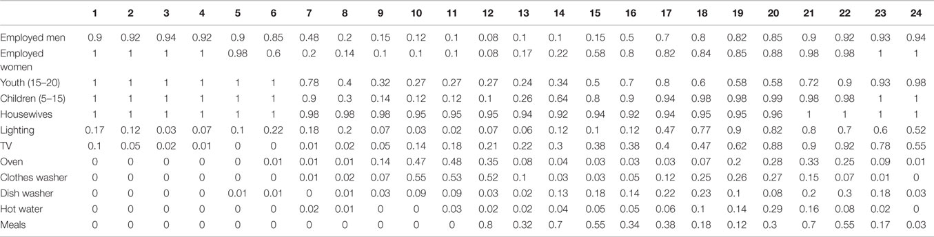
Table 5. Occupants’ living pattern and usage of some electric appliances during weekday, probabilities used in Eq. 35.

Table 6 provides the results of the total energy consumption, the furnace energy consumption, air-conditioning system electricity consumption, and other energy consumption on an annual basis. The furnace is assumed to have an energy efficiency of 0.85, and the air-conditioner has a COP of 2.0. The variables presented in the table are listed as follows: Φ = building azimuth, degree from due North; T = indoor air temperature; ACH = infiltration rate, taken as 0.15 for newly built house, and 0.5 for old house; SF = shading factor for window, 0 for no shading and 1.0 for complete shading; OF = opening factor for window, the opening area vs. the total area; N_light = number of light bulbs turned on each time; TT = total energy consumption, kWh; H = Furnace energy consumption; A/C = air conditioning consumption; O = other energy consumption. Those variables are chosen to find out the best building location, and the best occupants’ behaviors related to thermostat setpoint, window opening/shading, number of lighting turned on, and to find out the related impact on energy consumption.

TABLE 6

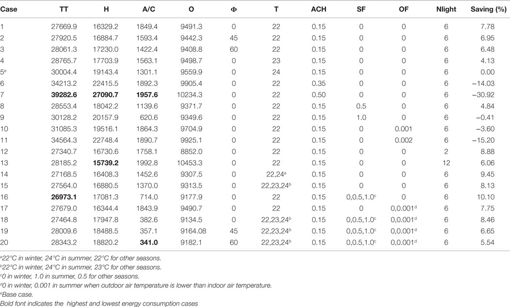
Table 6. Results for different cases.

When considering case No. 5 as the base case, the simulation results predicted energy saving of 4.1–10.1% in residential end-use energy consumption. The least energy consumption is case No.16 by applying 0% shading in winter, 50% shading during the transition season, and 100% shading in summer. Case No. 14 becomes the second to least energy consumer by raising the thermostat setpoint from 22°C to 24°C in summer. Case No. 13 has the lowest heating energy consumption because more lighting was turned on which generates additional heating in winter, and also a lower thermostat setpoint of 22°C was used in winter.

Case No. 20 has the lowest A/C energy consumption as it applies the following strategies: (1) changing thermostat setpoint throughout the year (22°C in winter, 23°C during transition season, and 24°C in summer); (2) applying 0% shading in winter, 50% shading during the transition season, 100% shading in summer; and (3) opening the window in summer when outside air temperature is lower than the room temperature. When windows are opened in winter, the heating energy consumption increases dramatically, as shown in case No.11.

From the comparison of case No. 5 in Table 6, it appears that the ventilation rate of the house has the greatest impact on the heating energy consumption, and the shading schemes appear to have the greatest impact on the A/C energy consumption. The optimum building azimuth is zero, with the front wall facing south. The electricity consumption of the A/C can be reduced by shading the windows, by opening them in summer (when the outdoor air temperature is below the indoor air temperature), and by employing a slightly higher thermostat setpoint temperature in summer and during transitional seasons.

Table 7 presents the percentage of energy consumption for each component of all the tested cases. It is shown that the furnace energy consumption accounts for 56–69%, and the A/C consumes 1.2–6.7%, lighting and electrical appliances consume 11–19%, hot water consumes 9.5–12%, and fans, including the exhaust fan and the blower fan of the furnace, account for 5.2–7.1% of the total energy consumption. Least amount of heating energy consumption and A/C consumption were found in Case No. 13 and case No. 20, the same as being observed in Table 5.

TABLE 7

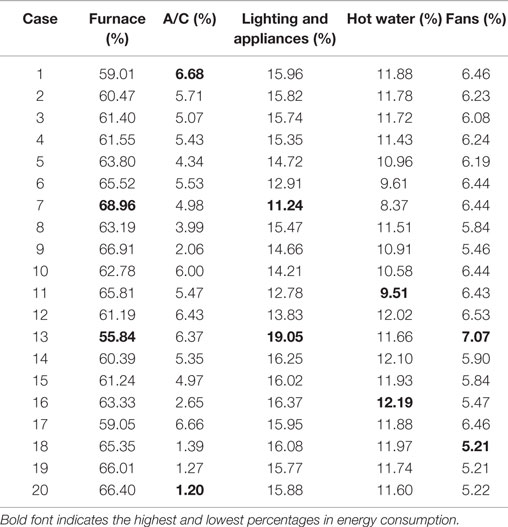
Table 7. Percentage of energy consumption for each component.

The accumulative energy consumption of the house was found to have a linear relationship with the accumulative degree days (adding all the degree days from the first day to the last day for calculation of the energy consumption) (Figure 9) regardless of the changes in occupants’ behaviors. The R² value was 0.99 and the relative difference between the predicted energy consumption from the correlation model and the simulation results was <7.6%. This appears to suggest that the occupants’ behavior has a linear impact on the building energy performance which deserves further investigation in order to develop simpler modeling algorithms of occupants’ behavior that could be easily integrated into existing building performance simulation programs.

FIGURE 9

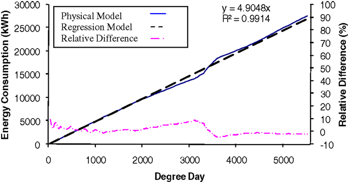
Figure 9. Regression model derived from the simulation results, case no. 11.

The simulation then is applied to the 270 houses in Oshawa which were monitored by smart meters. The ranges for the thermal resistance for the roofs, external walls, floors, and windows are 0.54–7.05, 0.64–3.11, 0.56–5.01, and 0.2–0.46 m² K/W, respectively. The ACH for those house ranges from 0.0745 to 0.744. The efficiency for heating ranges from 0.76 (furnace) to 2.0 (HP, estimated), for domestic hot water is from 0.55 to 0.82. The SEER for the AC units is from 6 to 10. The savings due to improvement of occupants’ behaviors is predicted to be from 6.8 to 11% of the total building energy consumption (Table 8). The improvement of occupants’ behaviors includes lowering the thermostat setpoint by 2°C in winter, provide full shading in summer, and close the window fully in winter, and turn off more lights in summer when not needed.

TABLE 8

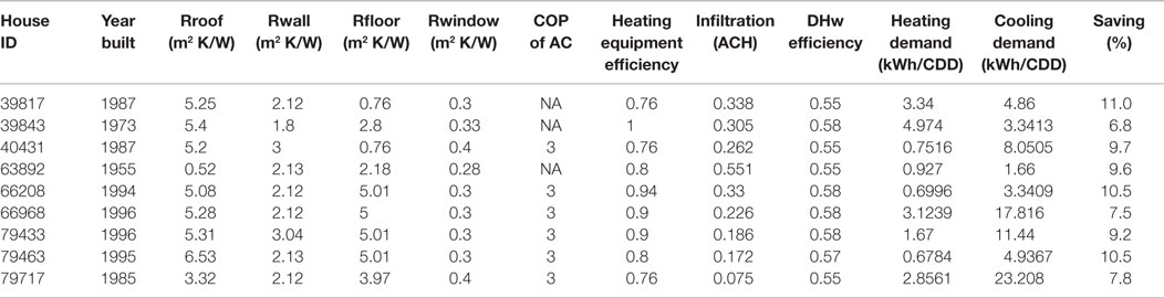
Table 8. Savings due to improve of occupants’ behaviors from selected house in Oshawa.

Conclusion

This paper presented a mathematical model that considers the building envelop, window shading, and opening schemes, and thermostat setpoint temperature and also usage pattern of the electric appliances, e.g., the impact on energy consumption and power demand due to different occupants’ behaviors related to window opening and shading schemes against the temperature and solar radiation, thermostat adjusting against the outdoor air temperature, and occupants’ preference on using the electrical appliances can be simulated. The results from the computer model are validated with ESP-r, a detailed CFD model and with the experimental measurement with good agreements.

The simulation results showed that the infiltration/ventilation rate of the house has the greatest impact on the heating energy consumption, and the shading schemes have the greatest impact on the A/C energy consumption. The electricity consumption of the A/C can be significantly reduced by appropriately applying window shading and opening schemes and by controlling the thermostat setpoint temperature. Keeping windows closed in winter and allowing solar radiation to be transmitted through them greatly help to reduce the heating loads of the house. This model can also be used for assisting the efficient building design and retrofit analysis since it take into account many factors such as building orientation, building envelop material, shading, as well as control on heating and cooling.

However, it is noted that as the study is only conducted in the house of Oshawa. The results might be different for houses located in other climate zones. Future work includes (1) development of simpler modeling algorithms of occupants’ behavior that could be easily integrated into existing building performance simulation programs; (2) incorporation of occupants’ attitude, social, economic and cultural behavior factors into the computer model.

Conflict of Interest Statement

The authors declare that the research was conducted in the absence of any commercial or financial relationships that could be construed as a potential conflict of interest.

Acknowledgments

The authors acknowledge the financial support from Natural Resources Canada, Oshawa Public Utility Corporation, Ontario Center for Excellence, and from the Faculty of Engineering and Applied Science of University of Ontario Institute of Technology.

Footnotes

1. ^http://apps1.eere.energy.gov/buildings/energyplus/?utm_source=EnergyPlus&utm_medium=redirect&utm_campaign=EnergyPlus%2Bredirect%2B1
2. ^http://www.esru.strath.ac.uk/Programs/ESP-r.htm
3. ^http://www.doe2.com/equest/
4. ^http://www.designbuilder.co.uk/
5. ^http://apps1.eere.energy.gov/buildings/energyplus/cfm/weather_data3.cfm/region=4_north_and_central_america_wmo_region_4/country=3_canada/cname=CANADA

References

Al-Mumin, A., Khattab, O., and Sridhar, G. (2003). Occupants’ behavior and activity patterns influencing the energy consumption in the Kuwaiti residences. Energy Build. 35, 549–559. doi: 10.1016/S0378-7788(02)00167-6

CrossRef Full Text | Google Scholar

Andersen, R. V., Toftum, J., Andersen, K. K., and Olesen, B. W. (2009). Survey of occupant behavior and control of indoor environment in Danish dwellings. Energy Build. 41, 11–16. doi:10.1016/j.enbuild.2008.07.004

CrossRef Full Text | Google Scholar

Asfour, O. S., and Gadi, M. B. (2007). A comparison between CFD and network models for predicting wind-driven ventilation in buildings. Build. Environ. 42, 4079–4085. doi:10.1016/j.buildenv.2006.11.021

CrossRef Full Text | Google Scholar

ASHRAE. (1992). Cooling and Heating Load Calculation Manual, 2nd Edn. Atlanta, GA: American Society of Heating, Refrigerating, and Air-Conditioning Engineers, Inc.

Google Scholar

Bourgeois, D., Reinhart, C., and Macdonald, I. (2006). Adding advanced behavioural models in whole building energy simulation: a study on the total energy impact of manual and automated lighting control. Energy Build. 38, 814–823. doi:10.1016/j.enbuild.2006.03.002

CrossRef Full Text | Google Scholar

Emery, A. F., and Kippenhan, C. J. (2006). A long term study of residential home heating consumption and the effect of occupant behavior on homes in the Pacific Northwest constructed according to improved thermal standards. Energy 31, 677–693. doi:10.1016/j.energy.2005.04.006

CrossRef Full Text | Google Scholar

Gunay, H. B., O’Brien, W., and Beausoleil-Morrison, I. (2013). A critical review of observation studies, modeling, and simulation of adaptive occupant behaviors in offices. Build. Environ. 70, 31–47. doi:10.1016/j.buildenv.2013.07.020

CrossRef Full Text | Google Scholar

Herkel, S., Knapp, U., and Pfafferott, J. (2008). Towards a model of user behavior regarding the manual control of windows in office buildings. Build. Environ. 43, 588–600. doi:10.1016/j.buildenv.2006.06.031

CrossRef Full Text | Google Scholar

Hong, T., D’Oca, S., Turner, W. J. N., and Taylor-Lange, S. C. (2015). An ontology to represent energy-related occupant behavior in buildings. Part I: introduction to the DNAs framework. Building Environ. 92, 764–777. doi:10.1016/j.buildenv.2015.02.019

CrossRef Full Text | Google Scholar

Iwashita, G., and Akasaka, H. (1997). The effects of human behavior on natural ventilation rate and indoor air environment in summer – a field study in Southern Japan. Energy Build. 25, 195–205. doi:10.1016/S0378-7788(96)00994-2

CrossRef Full Text | Google Scholar

Jian, Y. W., Guo, Y. J., Liu, J., Bai, Z., and Li, Q. G. (2011). Case study of window opening behavior using field measurement results. Build. Simul. 4, 107–116. doi:10.1007/s12273-010-0012-5

CrossRef Full Text | Google Scholar

Juodis, E., Jaraminiene, E., and Dudkiewicz, E. (2009). Inherent variability of heat consumption in residential buildings. Energy Build. 41, 1188–1194. doi:10.1016/j.enbuild.2009.06.007

CrossRef Full Text | Google Scholar

Lee, Y. S., and Malkawi, A. M. (2014). Simulating multiple occupant behaviors in buildings: an agent-based modeling approach. Energy Build. 69, 407–416. doi:10.1016/j.enbuild.2013.11.020

CrossRef Full Text | Google Scholar

Lin, Y., and Zmeureanu, R. (2008). Three-dimensional thermal and airflow (3D-TAF) model of a dome-covered house in Canada, Renew. Energy 33, 22–34. doi:10.1016/j.renene.2007.02.002

CrossRef Full Text | Google Scholar

Madhavi, I. (2010). Adaptive use of natural ventilation for thermal comfortin Indian apartments. Build. Environ. 45, 1490–1507. doi:10.1016/j.buildenv.2009.12.013

CrossRef Full Text | Google Scholar

Maier, T., Krzaczek, M., and Tejchman, J. (2009). Comparison of physical performances of the ventilation systems in low-energy residential houses. Energy Build. 41, 337–353. doi:10.1016/j.enbuild.2008.10.007

CrossRef Full Text | Google Scholar

McQuiston, F. C., Parker, J. D., and Spitler, J. D. (2000). Heating, Ventilating and Air Conditioning, Analysis and Design. New York, NY: John Wiley & Sons, Inc.

Google Scholar

Newsham, C. R. (1997). Clothing as a thermal comfort moderator and the effect on energy consumption. Energy Build. 26, 283–291. doi:10.1016/S0378-7788(97)00009-1

CrossRef Full Text | Google Scholar

Nicol, J. F., and Humphreys, M. A. (2004). A stochastic approach to thermal comfort – occupant behavior and energy use in buildings. ASHRAE Trans. 110, 554–568.

Google Scholar

Paatero, J. V., and Lund, P. D. (2006). A model for generating household electricity load profile. Int. J. Energy Res 30, 273–290. doi:10.1002/er.1136

CrossRef Full Text | Google Scholar

Page, J., Robinson, D., Morel, N., and Scartezzini, J. L. (2008). A generalised stochastic model for the simulation of occupant presence. Energy Build. 40, 83–98. doi:10.1016/j.enbuild.2007.01.018

CrossRef Full Text | Google Scholar

Papakostas, K. T., and Sotiropoulos, B. A. (1997). Occupational and energy behavior patterns in Greek residences. Energy Build. 26, 207–213. doi:10.1016/S0378-7788(97)00002-9

CrossRef Full Text | Google Scholar

Press, W. H., Teukolsky, S. A., Vetterling, W. T., and Flannery, B. P. (1992). Numerical Recipes in Fortran: The Art of Scientific Computing, 2nd Edn. Cambridge: Cambridge University Press.

Google Scholar

Reinhart, C. F. (2004). Lightswitch-2002: a model for manual and automated control of electric lighting and blinds. Sol. Energy 77, 15–28. doi:10.1016/j.solener.2004.04.003

CrossRef Full Text | Google Scholar

Rijal, H. B., Tuohy, P., Humphreys, M. A., Nicol, J. F., Samuel, A., and Clarke, J. (2007). Using results from field surveys to predict the effect of open windows on thermal comfort and energy use in buildings. Energy Build. 39, 823–836. doi:10.1016/j.enbuild.2007.02.003

CrossRef Full Text | Google Scholar

Shimoda, Y., Asahi, T., Taniguchi, A., and Mizuno, M. (2007). Evaluation of city-scale impact of residential energy conservation measures using the detailed end-use simulation model. Energy 32, 1617–1633. doi:10.1016/j.energy.2007.01.007

CrossRef Full Text | Google Scholar

Tanimoto, J., Hagishima, A., and Sagara, H. (2008). Methodology for peak energy requirement considering actual variation of occupants’ behavior schedules. Build. Environ. 43, 610–619. doi:10.1016/j.buildenv.2006.06.034

CrossRef Full Text | Google Scholar

Appendix

Nomenclature

A_i = area of the opening, m²;

A_j = inside wall/window surface area, m²;

AVG_i = average power input per cycle of the i^th electric appliance, W;

c_pi = specific heat of the i^th layer of the wall/floor/roof, J/kg K;

C_c = consumption coefficient, kWh/K;

C_d = flow coefficient, taken as 0.83, dimensionless;

C_f = draft coefficient, the actual pressure difference divided by the theoretical pressure difference, dimensionless;

C_h = consumption coefficient for heating, kWh/K;

C_p,a = Cp value of the inside surface, dimensionless;

C_p,i = Cp value at the i^th window surface, dimensionless;

CDD = cumulative degree days, °C;

dx_i = thickness of the i^th layer of the wall/floor/roof, m;

E_DHW = primary energy consumption of natural gas by the gas-fired hot water tank, J;

E_furnace = primary energy consumption of natural gas by the gas-fired furnace, J;

E_total = end-use energy need of the house, J;

E_pp = primary energy consumption by the power plant, J;

f_d,k = frequency of daily usage for an electric appliance in a group, e.g., 0.31 for clothes washer and 0.11 for clothes dryer;

f_h,i = hourly probability on the usage of the electric appliance, dimensionless;

Gd = diffuse solar radiation, W/m²;

GD = direct solar radiation, W/m²;

h = height to calculate the pressure difference, m;

h_win,in = combined convective coefficient over the inside surface of the window; W/m² K;

h_win,o = combined convective coefficient over the outside surface of the window, W/m² K;

H = height of the window, m;

k_i = thermal conductivity of the i^th layer of the wall/floor/roof/window, W/m⋅K;

m_i = air flow rate through the i^th opening, kg/s;

n = flow exponent, 0.5 for turbulent flow, dimensionless;

N = number of openings, dimensionless;

OF_i = opening factor, the opening proportional to the total window area, dimensionless;

p_o = ambient air pressure, Pa;

P_i,j = power input to the i^th electric appliance in phase j (e.g., ramp up, normal operation, ramp down), W;

q_abs,sol,in = absorbed solar radiation over the inner layer surface, W/m²;

q_abs,sol,out = absorbed solar radiation over the outer layer window surface, W/m²;

q_conv,l,in = convective heat flux over the inside wall/floor/roof/window surface, W/m²;

q_conv,l,out = convective heat flux over the outside wall/floor/roof/window surface, W/m²;

q_igh,in = internal heat gain over the window surface, W/m²;

q_rad,ihg,1 = radiation heat flux due to internal heat gain, W/m²;

q_sol,l,int = absorbed solar radiation at the inside wall/floor/roof surface, W/m²;

q_sol,l,out = absorbed solar radiation at the outside wall/floor/roof surface, W/m²;

q_surf,l,out,t = net surface-to-surface radiation leaving the outside wall/floor/roof/window surface, W/m²;

q_surf,l,in = net surface-to-surface radiation leaving the inside wall/floor/roof/window surface, W/m²;

q_win = heat transfer through the window, W/m²;

Q_ac = air-conditioning load, W;

Q_inf = heat loss/gain through exfiltration/infiltration, W;

QE = electricity consumption, kWh;

Q_furnace = furnace heating load, W;

Q_HVAC = heat addition rate by the heating system, W;

Q_{internal,conv} = convective part of internal heat gain from people, lighting, and electric appliances, W;

R_a = gas constant for air, J/kg K;

R_w = thermal resistance of the double pane, m² K/W;

SF = window shading factor, 0 indicates no shading, and 1.0 indicates complete shading, dimensionless;

t = time, s;

th = thickness of the wall/floor/roof, m;

T = temperature of the wall/roof/floor, K;

T_a = indoor air temperature, °C;

T_is = inner layer temperature of the window,°C;

T_j,in = temperature of inside surface j, °C;

T_o = outside air temperature, °C;

T_os = outer layer temperature of the window, °C;

U = building consumption factor, kWh/K;

U_w is the U-factor of the double pane, W/m² K;

v_w = wind speed over the window surface, m/s;

W = width of the window, m;

W_app = electric power input to the electric appliances, W;

W_blower = electric power input to the blower fan of the furnace, W;

W_comp = electric power input to the compressor of the AC, W;

W_exhaust = electric power input to the exhaust fan, W;

W_i = electric input of the i^th electric appliance, W;

x = length, m;

α_{diffuse,inner} = absorbance of diffuse solar radiation at the inner layer surface, dimensionless;

α_{diffuse,outer} = absorbance of diffuse solar radiation at the outer layer surface, dimensionless;

α_Direct,inner = absorbance of beam solar radiation at the inner layer surface, dimensionless;

α_Direct,outer = absorbance of beam solar radiation at the outer layer surface, dimensionless;

α_h = temperature diffusion coefficient for each layer of the wall, m²/s;

ρ = out flow air density, kg/m³;

ρ_a = density of the outflow air, kg/m³;

ρ_i = density of the i^th layer of the wall/floor/roof/window, kg/m³;

ρ_o = outdoor air density, kg/m³;

τ_j = time required for phase j, min.;

Δp_i = pressure difference between the house and the outdoor air, Pa;

Δp_p = pressure difference due to building pressurization, assumed zero in this paper, Pa;

Δp_s = stack effect pressure difference, Pa;

Δp_w,i = wind induced pressure difference, Pa;