Volcano-tectonic interactions revealed by inversion of focal mechanisms: stress field insight around and beneath the Vatnajökull ice cap in Iceland

Introduction

At the intersection of the North Atlantic spreading ridge and the Icelandic hotspot, Iceland is a particularly interesting area to investigate the interactions in space and time between tectonics and volcanic activity. The central part of the island is of critical interest because it is formed by the most active volcano-tectonic systems. Moreover, two-thirds of the area is covered by the Vatnajökull ice cap (Figures 1A,B) and is also featured by the fastest rebounding process.

FIGURE 1

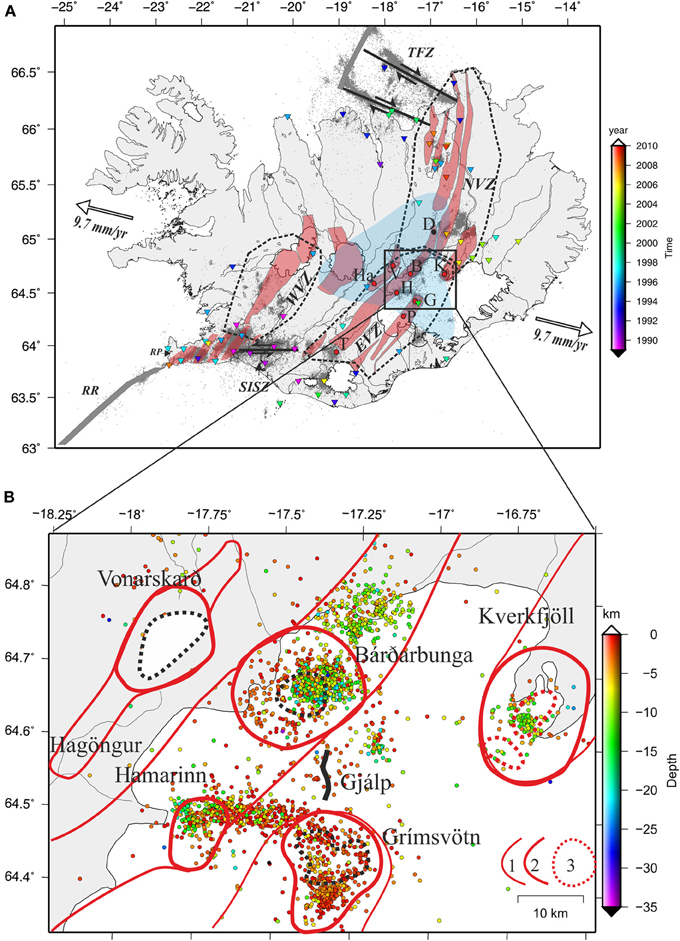
Figure 1. Location of the studied area and the geodynamic context of the central part of Iceland. (A) Rift and transform zones in Iceland. Thick gray lines: offshore ocean ridge axes of the Mid-Atlantic ridge. Thick black lines: transform zones with couple of arrows indicating the sense of movement (modified after Angelier, 2002). Main Holocene volcanic systems of onshore rift zones in red with glacier left in white (after Sæmundsson, 1979; Thordarson and Larsen, 2007). Earthquakes epicenters from 1991 to 2009 provided by IMO are shown as small black dots. Apex zone of Icelandic hotspot superimposed in light blue (after Tryggvason et al., 1983). Triangles: seismic station locations, colored as a function of the time of installation (see color bar on the right side). Red dots: active central volcanoes belonging to the volcanic systems. B: Bárðarbunga; D: Dyngjufjöll-Ytri; G: Grimsvötn; H: Hamarinn; Ha: Hagöngur; K: Kverkfjöll; Ka: Katla; P: Þórðarhyrna; V: Vonarskarð. (B) Area of study showing the epicenters of the dataset used for the inversion (2434 mechanisms) as function of depth, and the volcanic systems. 1:fissure swarm; 2: domain of central volcano; 3: caldera (after Jóhannesson and Sæmundsson, 1998).

Using a large number of focal mechanisms provided by the Icelandic Meteorological Office (IMO), we computed a first order stress field to characterize the crustal stress. This stress field results from volcanic, tectonic processes and isostasic rebound of the crust. Episodic volcanic crises may also cause local high diversity of focal mechanisms with time (e.g., Einarsson, 1991; Roman et al., 2008; White et al., 2011). Thus, a second stress analysis was carried out to evaluate the state of stress during a volcanic crisis and the results were compared to the regional stress field.

In this paper, a regional stress field that includes (1) a checkerboard test to evaluate the sensitivity of random choice of the nodal plans of double focal solutions and the confidence in the dimension of the selected subareas, (2) an analysis of the different damped stress fields obtained by the Hardebeck and Michael (2006) approach in terms of stress orientations and stress regime, (3) the stability of the resulting stress field by an analysis of random errors propagated in the data is carried out over a 20 year time-span. Another “local” stress inversion is effected during a volcanic crisis using a random stress search. Finally, we discuss the resulting stress field (regional and as a function of time) in the light of recent volcano-tectonic and crustal rebound modeling to decipher the probable causes not only of stress orientations but also of stress magnitudes in regard to volcanic, tectonic and the potential influence of the Vatnajökull ice cap, and their implications for the comprehension of the slow spreading ridge.

Geodynamic Context

Geodynamic Context of Iceland

Iceland is an emerged part of the Mid-Atlantic Ridge originated by the superposition of the spreading ridge axis and the Icelandic hotspot (Figure 1A). This particular situation gives rise to interactions between tectonic and volcanic processes, intimately linked in such a region. On the Earth's surface, these interactions are expressed by volcano-tectonic systems made of central volcanoes, long eruptive and non-eruptive fissures and faults (Sæmundsson, 1979). Moreover, Iceland is undergoing glacial isostatic adjustment due to the recent retreat of the glacier (Árnadóttir et al., 2009).

The Icelandic rift consists of several volcano-tectonic systems grouped into the Eastern Volcanic Zone (EVZ), the Western Volcanic Zone, and the North Volcanic Zone (Figure 1A). A typical volcano-tectonic system consists of a central volcano associated with eruptive fissures, normal faults and extension fractures. The Icelandic mantle plume of the hotspot lies under the central part of Iceland, which is partly covered by the Vatnajökull glacier (e.g., Tryggvason et al., 1983; Allen et al., 2002). Plate divergence occurs at a rate of approximately 2 cm.year⁻¹ in a N105°E direction (DeMets et al., 1990, 1994). The Iceland rift is offset by two active transform zones: the South Iceland Seismic Zone and the Tjörnes Fracture Zone, connecting the emerged part of the rift to the offshore Reykjanes and Kolbeinsey ridges, respectively.

Geological Setting of the East Volcanic Zone

The volcano-tectonic systems

Our study area in the central and eastern parts of the EVZ is two-thirds covered by the Vatnajökull ice cap (Figures 1A,B), explaining why the knowledge of its geology is much less detailed than that of ice-free regions of volcanic zones. Four volcanic systems have been identified in the EVZ: Grimsvötn-Laki, Bárðarbunga-Veiðivötn, Vonarskard-Hagöngur and Kverkfjöll. (1) The Grimsvötn-Laki volcanic system extends from the Laki volcanic fissure (ice-free domain, south of the Vatnajökull) to the Þórðarhyrna and Grimsvötn central volcanoes (ice-covered). In the two last decades, the Grimsvötn volcano has been the most active volcano in Iceland (Larsen et al., 1998; Larsen, 2002); the most recent eruptions occurred in 1998, 2004, and 2011. (2) Bárðarbunga-Veiðivötn is a large volcanic system roughly 180 km long. It extends from the edge of the Torfajökull central volcano at its southwestern part to the Dyngjufjöll-Ytri hyaloclastite ridge at its northeastern part. It comprises the Bárðarbunga, a large ice-covered central volcano, together with the Hamarinn central volcano that lies 15 km southwest of Bárðarbunga. This volcanic system is characterized by numerous fissure swarms (eruptive and non-eruptive) trending NE-SW, presumably extending through the margins of the glacier (Jóhannesson and Sæmundsson, 1998). The Bárðarbunga central volcano was considerably active during historical times. (3) The Vonarskard-Hagöngur, situated northwest of the Bárðarbunga-Veiðivötn volcanic system, is a volcano-tectonic system in which the main central volcano is Vonarskard-Tungnafellsjökull. (4) The Kverkfjöll volcanic system, around the Kverfjöll central volcano, belongs to the North Volcanic Zone.

The crustal structure

Only a few seismic profile images show the crustal structure beneath the Bárðarbunga-Grimsvötn volcanic complex (Darbyshire et al., 1998, 2000; Allen et al., 2002). The upper crust is believed to be thin below this area, being only about 4–5 km thick, while the Moho reaches a depth of roughly 40 km directly above the plume center and thins rapidly away from it (Darbyshire et al., 1998, 2000; Allen et al., 2002). A recent study based on gravity data has shown that the Vonarskard, Bárðarbunga, Kverkfjöll and Grimsvötn volcanoes are associated with major high density anomalies located in the upper crust (Guðmundsson and Hognadóttir, 2007), interpreted as predominantly basic intrusions. Note that, in contrast, no gravity anomaly is observed for the Hamarinn central volcano.

Associated seismicity

More than 240,000 earthquakes with seismic moment magnitude Mw ranging from −2.4 to 6.4 were recorded locally between 1990 and 2010 by the IMO seismological network; they cluster mainly around the transform zones (Figure 1A). Other large clusters of earthquakes are observed around some of the central volcanoes, particularly in the EVZ, which includes the youngest and most active volcanic systems of Iceland (Figure 1B).

Materials and Methods

Focal mechanisms are commonly used to investigate the crustal stress in tectonically active regions. However, determining the stress field from focal mechanisms is not straightforward and raises several questions: what is the volume in which crustal stress can be considered to be homogeneous? What is the number and quality of the required data? How can the presence of different types of focal mechanisms within the volume and the geometry of the active tectonic systems be explained? Paleostress analyses highlighted that the separation of a heterogeneous dataset into spatially and temporally homogeneous subsets is fundamental to avoid artefacts in stress solutions: such computed solutions can only represent a compromise between different homogeneous subsets and hence are inconsistent with the actual stress field (e.g., Célérier et al., 2012). Automatic and interactive separations to obtain homogeneous subsets have been performed for paleostresses (e.g., Armijo and Cisternas, 1978; Angelier, 1979; Angelier and Manoussis, 1980; Etchecopar et al., 1981; Etchecopar, 1984; Mercier and Carey-Gailhardis, 1989; Yamaji, 2000, 2003). However, such automatic methods may give rise to serious artefacts (Angelier, 1984; Lisle and Vandycke, 1996; Delvaux and Sperner, 2003; Liesa and Lisle, 2004; Sperner and Zweigel, 2010). The most robust way forward is to separate the data based on fault kinematics, mechanical consistency and field observations (e.g., Bergerat, 1987), but this is not feasible when the dataset consists of hundreds or thousands of focal mechanisms.

Hardebeck and Michael (2006) proposed a stress inversion method that finds the least complex stress field model consistent with the data. This uses an adaptive damping method, which discriminates between variations that are or are not strongly required by the data and retains only variations that are well-resolved. In more detail, the area studied is divided into subareas and all cells are simultaneously inverted for the reduced stress tensor while minimizing the stress differences between adjacent areas. This method involves a random choice of nodal plan during the inversion procedure, which is especially useful when using a large catalog of focal mechanisms such as in this study. We will retain this methodology to define a preliminary stress field and its significance in terms of volcano-tectonic processes beneath the central part of Iceland (Figure 1A). Regarding the state of stress over time, a random stress search is more suitable for smaller data subsets than the regional damping method, and it will be carried out here for a volcanic crisis.

The Earthquake Catalog Used for Inversion

In the area studied, 5997 earthquakes with moment magnitudes from −2.3 to 5.4 M_w were recorded in the IMO database from 1991 to 2009 and each of these events was associated with a double-couple focal mechanism. An estimation of the fault plane solution is based on P and S polarities and amplitude data (Rögnvaldsson and Slunga, 1993, 1994). Fault plane solutions and earthquake location are refined interactively by checking the arrival times of seismic events issued from the network routine (Böðvarsson et al., 1996). Single-event and multi-event locations are used in the routine analysis. Where the station coverage is good, the optimal fault plane solution can be expected to be within ±15° of the three source angles for events not larger than 0.5 Mw (Rögnvaldsson and Slunga, 1993). Quality and accuracy of these solutions improved during the last decade due to the increase in station coverage. However, the area we studied is located in the central part of Iceland and is less densely covered than the transform zones, partly due to the presence of the glacier. We selected events with magnitudes greater than 2 M_w (2434 mechanisms; Figure 1B) to remove earthquakes that were detected by too few stations and so were poorly determined. The earthquakes selected cluster mainly around central volcanoes at depths ranging from 12 to 8 km for Bárðarbunga and Kverkfjöll, and 8 km to near the surface for Hamarinn and Grimsvötn (Figure 1B).

Stress Inversion Principle

The stress inversion method is based on the assumption that the slip vector $\overrightarrow{s}$ (defined by the rake) is parallel to the shear stress $\overrightarrow{\tau }$ as described by Wallace (1951) and Bott (1959). These authors assumed that the direction of slip on a fault plane is parallel to that of the resolved shear stress. Instead of using the absolute magnitude of the stress tensor, a reduced stress tensor is sought by subtracting an isotropic part and a scale factor that do not affect the orientation of the resolved shear stress $\overrightarrow{\tau }$ (e.g., see appendix of Burg et al., 2005). Thus, the reduced stress tensor T_r is defined by the orientation of the principal stress axes $\overrightarrow{\sigma }$₁, $\overrightarrow{\sigma }$₂, and $\overrightarrow{\sigma }$₃ (with stress magnitudes of σ₁ ≥ σ₂ ≥ σ₃, respectively) and the stress shape ratio $\Phi =\left(\frac{{\sigma }_2-{\sigma }_3}{{\sigma }_1-{\sigma }_3}\right)$ as defined by Angelier (1975), represented in the principal frame S = ($\overrightarrow{\sigma }$₁, $\overrightarrow{\sigma }$₂, $\overrightarrow{\sigma }$₃) where $\overrightarrow{\sigma }$₁, $\overrightarrow{\sigma }$₂, and $\overrightarrow{\sigma }$₃ are unit vectors such as:

$\begin{array}{cc}{\text{ T}}_r^S=\left(\begin{array}{ccc}1& 0& 0\\ 0& \Phi & 0\\ 0& 0& 0\end{array}\right)& (1)\end{array}$

Two types of algorithm are used here: (1) a linear stress inversion, which minimizes the difference between $\overrightarrow{s}$and $\overrightarrow{\tau }$ implemented in the damped stress inversion (Michael, 1984, 1987; Hardebeck and Michael, 2006) and (2) a random stress search such as Etchecopar et al. (1981) and Etchecopar (1984) implemented in the Fsa package (Célérier, 2013), which minimizes the angular α misfit between $\overrightarrow{\tau }$ and $\overrightarrow{s}$. For more details pertaining to the minimization criteria, the reader is referred to the review of Célérier et al. (2012). The first algorithm is used to determine the regional stress field using all the dataset. The second is used to detect the mechanically homogenous data subset when less data are considered for inversion, such as during a volcanic eruption. In this way, the compatibility of the stress tensor can be verified with each datum. For double-couple focal mechanisms, an ambiguity of the two nodal planes arises because the shear stress (τ) and the slip (s) cannot be aligned on both nodal planes, unless a principal stress axis is parallel to the B axis or the stresses are axially symmetric such that Φ is close to 0 or 1 (Gephart, 1985). Following the procedure of Hardebeck and Michael (2006), we adopted a random choice of the nodal plane in the inversion process. In the following section, we will discuss the implications of this choice. For the random stress search, the fault plane yielding the lowest α misfit between the two nodal planes is considered for inversion (i.e., the best fault plane).

Damped Stress Inversion

We argue that the stress field is a function that can vary gradually from one point to another due to local forces superimposed on the regional tectonic stress. To take into account this progressive variation, we assume that the stress tensor computed for the area just around the point of coordinates x, y, and z is due to mechanical local conditions existing at this point, but is also influenced by tectonic conditions of the neighboring volume (x ± ε, y ± ε, z ± ε). The region studied is divided into a series of cells and the dataset (in our case the focal mechanism parameters) is partitioned in this mesh. In each cell, if the number of data is sufficient, it is theoretically possible to invert the local stress tensor as explained above. We invert simultaneously all the tensors for all the cells using the classical equation of tomography techniques given by:

$\begin{array}{cc}{G}_{all}{m}_{all}=d_{all}& (2)\end{array}$

Where d_all is the data matrix (slip vector and plane orientation for each focal mechanism) and m_all the model matrix containing the stress tensors which is defined by 5 parameters (see details in Hardebeck and Michael, 2006). G_all is derived from the data of each focal mechanism at node ij and is given by:

$\begin{array}{cc}{G}_{all}=\left(\begin{array}{ccccc}{G}_{11}& & & & 0\\ & G_{21}& & & \\ & & G_{31}& & \\ & & & \dots & \\ 0& & & & G_{ij}\end{array}\right)& (3)\end{array}$

At least a square solution for this system is given by:

$\begin{array}{cc}{G}_{all}^{\text{T}}{G}_{all}{m}_{all}=G_{all}^{\text{T}}{d}_{all}& (4)\end{array}$

This inversion provides the same results as if the data for each cell were inverted separately. To damp the differences in the estimated stress tensor between neighboring cells, we introduce a matrix D, the same size as G, with identity matrices for neighboring cells and zeroes everywhere else Hardebeck and Michael (2006). The damped least square solution is then given by:

$\begin{array}{cc}\left\{G_{all}^T{G}_{all}+e^2{D}^{T}D\right\}{m}_{all}=G_{all}^T{d}_{all}& (5)\end{array}$

Where e is the scalar damping parameter that controls the relative weighting sum of the data misfit and the model variance (Figure 2A). Not only does this damping technique simultaneously minimize the misfit between the estimated stress field model and the data, it also minimizes the differences between the estimated stress tensors in neighboring cells (referred to as model variance). The computation is very close to the inversion techniques developed by Aki and Richards (1980) for arrival time tomography.

FIGURE 2

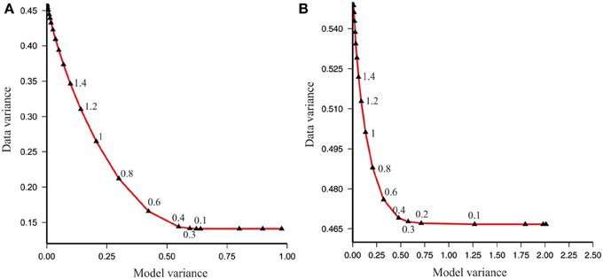
Figure 2. Trade-off curve between the data variance and the model variance for the full range of possible values of the damping parameter e. Number close to each black triangle denote the value e at this mark (Hardebeck and Michael, 2006). (A) Trade-off curve for inversion of the synthetic data; (B) Trade-off curve for inversion of the real data.

Random Stress Search

The random stress search is based on a Monte Carlo procedure and was developed for stress inversion by Etchecopar et al. (1981) and Etchecopar (1984). In this study, we used the Fsa package (Célérier, 2013). The best reduced stress tensor is obtained by testing a number of random stress tensors (here 10,000) and selecting those that yield the shear stress direction as close as possible to the observed slip vector of a data subset. The individual angular α misfit is defined as the absolute difference between the observed and predicted rake for each focal mechanism. The misfit function is thus defined by the average of the lowest individual misfit of the dataset.

Results

Regional Stress Inversion

Checkerboard tests

The checkerboard test is a very common technique in geophysics to evaluate the resolution and sensitivity of inversion results to the data. More specifically, we have designed a synthetic stress field as the model m containing a stress tensor at each node ij. We generated synthetic data d' based on the locations and fault planes of the earthquakes in the catalog and computed the new predicted slip vector for each focal mechanism k given by the model m. By inverting the data d', we obtained the model $\widehat{m}$ and we inspected the result by comparing the model m with $\widehat{m}$. The aim of the following tests is to evaluate the grid size and random choice of the actual fault plane proposed by Hardebeck and Michael (2006). No noise is added to the synthetic data.

We gridded the study area with a 2.5 × 2.5 km mesh to obtain on average 30 focal mechanisms per cell (Figure 3). Because earthquakes cluster under each central volcano and are located in a limited range of depth typical for each volcano, we adopted a 2D grid as a first order stress field (see Figures 1B, 3). We also performed experiments using different grid sizes such as 5 × 5 km and 1 × 1 km. The grid size of 2.5 × 2.5 km has the advantage of giving a high number of cells associated with a stress tensor to resolve kilometric stress deviation, while keeping an average of 25–30 focal mechanisms per cell, which is statistically relevant for a representative stress tensor. On the one hand, reducing the grid size significantly diminishes the average number of focal mechanisms per cell. On the other hand, taking a larger grid size increases the number of focal mechanisms per cell and decreases the number of computed stress tensors. In this case, the stress field is resolved but small stress variations would not be revealed.

FIGURE 3

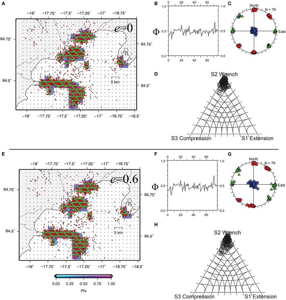
Figure 3. Checkerboard tests using synthetic earthquakes based on the selected earthquake catalog. (A–D) With no damping (e = 0): (A) map of the stress field issued from inversion of the synthetic earthquakes, superimposed red and green bars represent $\overrightarrow{\sigma }$₁ and $\overrightarrow{\sigma }$₃ respectively, denoting the strike slip regime; color bar denote the value of the stress shape ratio Φ from the stress inversion; epicenters of earthquakes are represented as red dots; the small crosses show the nodes of the grid in Figure 2B; (B) diagram of Φ with the number of the stress tensor on x-axis and the value of Φ on y-axis; (C) stereo-diagram of lower hemisphere (Schmidt's projection) showing the principal stresses where red, blue and green denote $\overrightarrow{\sigma }$₁, $\overrightarrow{\sigma }$₂, and $\overrightarrow{\sigma }$₃ respectively; (D) ternary diagram of the principal stress axes (e.g., Frohlich, 1992); (E–H) with damping (e = 0.6), same legend as for checkerboard test with no damping.

We produced a simple synthetic model m as the strike slip regime with $\overrightarrow{\sigma }$₁ alternatively heading to N 000° and N 045° for each adjacent node ij. Then, we ran two inversion tests with (1) no damping (e = 0) and (2) the optimal e-value of damping chosen at the lower left corner of the trade-off curve, which yields the best compromise between misfit and model variances (Figure 2A). Stress tensors are calculated if at least 8 focal mechanisms are contained per cell for both tests.

For inversion with no damping, the results show that the stress field $\widehat{m}$ issued from the inversion of the synthetic data gave a good reproduction of the synthetic stress field m in terms of stress orientations in all cells (Figure 3). The values of the fourth unknown Φ are on average also well-retrieved from the inversion. Examining the plunge of $\overrightarrow{\sigma }$₁, $\overrightarrow{\sigma }$₂, and $\overrightarrow{\sigma }$₃ on a triangular diagram (Figure 3D) shows that all stress tensors are strike-slip in type with $\overrightarrow{\sigma }$₂ within 20° of the vertical. This first test reveals that a random choice of the nodal planes does not significantly affect the resulting stress field. Thus, the size of the grid is well-adapted to the inversion.

For the next inversion, we used a value for the damping parameter e = 0.6, corresponding to the optimal value given by the trade-off curve depicted in Figure 2A. Figure 3 shows that the stress orientation of the principal axes is well reproduced with a damped stress inversion. Examining the plunge of $\overrightarrow{\sigma }$₁, $\overrightarrow{\sigma }$₂, and $\overrightarrow{\sigma }$₃ on a triangular diagram (Figure 3H) reveals that all stress tensors remain strike-slip in type, although more stress tensors show a $\overrightarrow{\sigma }$₂ away from the vertical than do the ones from the model with no damping. These results also reveal that cells containing a low number of data are first influenced by cells with a higher number of data when the damping parameter increases (Figure 3E).

These two checkerboard tests show that the sensitivity of the damped inversion is dependent on the number of data per cell and thus on the grid size. The synthetic stress field is well reproduced, despite the random choice among the two nodal planes. One should note that the heterogeneity of data within a cell is not evaluated with these tests.

Stress field results

We performed a damped stress inversion on the selected earthquake catalog described in section The Earthquake Catalog Used for Inversion. We used the grid size chosen from the checkerboard tests, as well as the same minimum number of focal mechanisms per cell to compute a stress tensor (Figure 3). Because the solution is not unique for such an inversion method, we computed four damped inversion models as a function of the scalar damping parameter e to evaluate the stability of the stress field in each cell. The e-values were chosen from the optimal value at the lower left corner of the trade-off curve (e = 0.6) compared to an a priori over-damped model (e = 1.4; Figure 2B).

Considering all the models, the effect of damping can clearly be seen in Figure 4, where a smoother model was obtained with high damping. All type of faulting were revealed, but normal and strike-slip faulting dominated (Figures 4, 5). In detail, the ternary diagrams show a continuum regime between strike-slip and normal faulting, revealing the occurrence of stress permutations between $\overrightarrow{\sigma }$₁ and $\overrightarrow{\sigma }$₂. This continuum is in agreement with the high stress shape ratio (e.g., Φ = 1) determined in the models (see Table 1). Nevertheless, stress permutation between $\overrightarrow{\sigma }$₂ and $\overrightarrow{\sigma }$₃ associated with a low stress shape ratio also occurs and this undergoes a slight decrease with the damped model e = 1.4. In a first approximation, the stress trajectory is rather scattered for the model e = 0.6. However, according to the geographical location, some trends remain stable irrespective of the e-value (Figure 4). Thus, the stress field can be divided into one of four bins as a function of the central volcano: Bárðarbunga (B), Grimsvötn (G), Kverkfjöll (K), or Hamarinn (H). For convenience, we calculated the minimum horizontal stress σ_hmin as defined by Lund and Townend (2007) to read the trend of the stress trajectory (Figure 6). (1) The σ_hmin in the H bin trends NW-SE with two main peaks at N135E and N090 for damping of e = 0.6. Upon increasing the damping e-value, the preferred orientation reaches N120 to N130. (2) The G bin shows more scattered $\overrightarrow{\sigma }$_hmin trends. However, the two main peaks are in the range of N060-90 and N000-N010. Damping tends to decrease the height of the first peak and to converge the $\overrightarrow{\sigma }$_hmin orientations toward a more narrow range between N070 and N080. (3) The stress pattern of the B bin is the most constant, showing a main peak in the range of N090 to N100, with few $\overrightarrow{\sigma }$_hmin axes tending perpendicular to this direction. When damping is strengthened, the main peak lies from N070 to N080. (4) The K bin constantly shows the same direction of $\overrightarrow{\sigma }$_hmin, which ranges from N010 to N030.

FIGURE 4

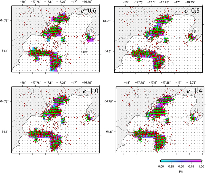
Figure 4. Results for different damped stress fields. The damping parameter e is indicated in each map. Same legend as Figure 3.

FIGURE 5

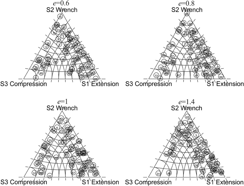
Figure 5. Ternary diagrams of the principal stress axes of the reduced stress tensors for the different damped stress fields. The damping parameter e is indicated above each diagram.

TABLE 1

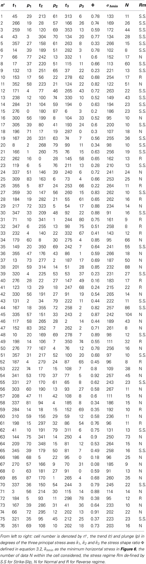
Table 1. Stress tensor solutions computed for a damping parameter e = 0.6, model displayed in Figure 4.

FIGURE 6

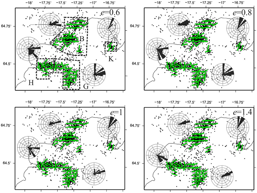
Figure 6. $\overrightarrow{\sigma }$_hmin maps for the different damped stress fields. The inset rose diagrams depict the direction of $\overrightarrow{\sigma }$_hmin in 10° bins for each volcano denoted by the capital letter and delimited by the dashed black line (only showed on the stress field for e = 0.6). Same background as for Figure 3.

When the scalar damping parameter e increases, the main stress trajectories are more clearly highlighted. This could suggest that the main tendency observed from the stress trajectories is statistically strongly required by the data, although some local perturbations are maintained even with a high damping as shown in Figure 6. Here, we only consider the trends that remain stable irrespective of the e-values. These correspond to a stress field strongly required by the data.

Error propagation tests

To evaluate the stability of stress inversion in each cell, we generated a data vector that includes random noise and inverted this to evaluate the propagation of the data errors. This experiment is similar to the “Monte Carlo” tests commonly used in seismic tomography.

To carry out error propagation tests with the damped stress field models determined in section Stress Field Results, we first added random perturbations on the strike, dip and rake of our dataset in the range of the uncertainties of the fault plane solution (±15°, section The Earthquake Catalog Used for Inversion), following a normal distribution (Figure 7D). We then inverted the noisy data and finally evaluated the difference between the noisy models and the optimum damped model (e = 0.6) determined in section Stress Field Results. A convenient way to evaluate error propagation is to compute the scalar product of the principal stresses between a perturbed stress tensor and a non-perturbed one at the ij cell, giving the angular deviations. For convenience, the angular deviation for each of the principal stresses is noted herein as $\overrightarrow{\sigma }$₁ − $\overrightarrow{\sigma }$^′₁, $\overrightarrow{\sigma }$₂ − $\overrightarrow{\sigma }$^′₂, and $\overrightarrow{\sigma }$₃ − $\overrightarrow{\sigma }$^′₃.

FIGURE 7

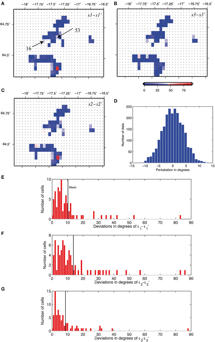
Figure 7. Results for error propagation tests. (A–C) represent the surface map of the angular deviation in degrees indicated by the color bar scale for $\overrightarrow{\sigma }$₁ − $\overrightarrow{\sigma }$^′₁, $\overrightarrow{\sigma }$₂ − $\overrightarrow{\sigma }$^′₂, and $\overrightarrow{\sigma }$₃ − $\overrightarrow{\sigma }$^′₃ respectively. Cells 53: example of stress axes permutation between $\overrightarrow{\sigma }$₁ and $\overrightarrow{\sigma }$₂ while $\overrightarrow{\sigma }$₃ remains unchanged (further explanation in text). Cell 16: example of large stress deviations for all of principal stress axes. (D) is the normal distribution of the errors used to perturb the data. (E–G) are histograms showing the distribution of the angular deviation as function of the number of cell.

The results are presented for each principal stress axis in Figure 7. The histograms in Figures 7E–G reveal the mean angular deviations associated with the mean errors in the range of 10 ± 13°, 14 ± 16°, and 9 ± 12° for $\overrightarrow{\sigma }$₁ − $\overrightarrow{\sigma }$^′₁, $\overrightarrow{\sigma }$₂ − $\overrightarrow{\sigma }$^′₂, and $\overrightarrow{\sigma }$₃ − $\overrightarrow{\sigma }$^′₃ respectively, showing relatively small deviations. Interestingly, $\overrightarrow{\sigma }$₃ is the most stable stress axis while $\overrightarrow{\sigma }$₂ is the least stable one. The number of cells with a deviation of under 10° for $\overrightarrow{\sigma }$₃ − $\overrightarrow{\sigma }$^′₃ is 59 (73% of the cells). The surface map deviations depicted in Figures 7A–C show that cells with high deviations (more than 25°) are systematically found on either a and c or b and c maps. For instance, cell 53 for $\overrightarrow{\sigma }$₂ − $\overrightarrow{\sigma }$^′₂ is associated with a high angular deviation that can also be found in the same cell for $\overrightarrow{\sigma }$₁ − $\overrightarrow{\sigma }$^′₁ but not for $\overrightarrow{\sigma }$₃ − $\overrightarrow{\sigma }$^′₃ (Figure 7). This suggests that stress rotation occurs around the $\overrightarrow{\sigma }$₃ stress axis, which remains the constant axis. Nevertheless, cell 16 is found to be deviated for all the principal stress axes (Figure 7). Stress deviations are therefore mainly expressed by rotations along one of the principal stress axes. It is not surprising that $\overrightarrow{\sigma }$₂ is the least stable stress axis since it is the common denominator for stress permutations such as $\overrightarrow{\sigma }$₁/$\overrightarrow{\sigma }$₂ and $\overrightarrow{\sigma }$₂/$\overrightarrow{\sigma }$₃. However, compared to the damped stress field models, we already pointed out the capacity of the stress field to permute mainly between $\overrightarrow{\sigma }$₁ and $\overrightarrow{\sigma }$₂ as shown on the ternary diagrams (Figure 5). So this stress permutation revealed through the stress field models is in good agreement with the results of the error propagation test. Applying tests with different damping parameter values (i.e., e = 0.8, 1, 1.4) yielded lower mean values concerning the deviation for each principal stress axis, keeping $\overrightarrow{\sigma }$₃ as the most stable axis. Adding larger noise, of the order of ±30° following a normal distribution, led to an increase in the mean angular deviation for each stress component of the order of 3°. Although more cells are disturbed, 44 cells for $\overrightarrow{\sigma }$₃ − $\overrightarrow{\sigma }$^′₃ have a deviation of under 10°, which represents 58% of all cells. Overall the error propagation tests show that the computed stress fields are stable.

State of Stress During the 1996 Volcanic Crisis

Several eruptions occurred during the 20 year time-span of the study. To select the eruptions associated with a large number of focal mechanisms for stress inversion purposes, a window of 100 earthquakes within 30 days was set up. Thus, only the volcanic crises in October 1996 (Guðmundsson et al., 2004, and references therein) and November 2004 in Grímsvötn (Sigmundsson and Guðmundsson, 2004) yielded significant numbers of earthquakes to carry out a proper analysis of state of stress (Figure 8A). Here, we focus on the volcanic crisis of 1996 because the resulting regional stress field shows only two main orientations of stress axes: (1) a dominant one nearly perpendicular to the spreading direction, and (2) a minor tendency in agreement with the spreading direction (Figure 6). The Grímsvötn area shows a more complex stress pattern that is probably not only related to volcano-tectonic interactions but also associated with a major geothermal activity (Bjórnsson et al., 1982, 1992) and outburst (i.e., jökulhlaup).

FIGURE 8

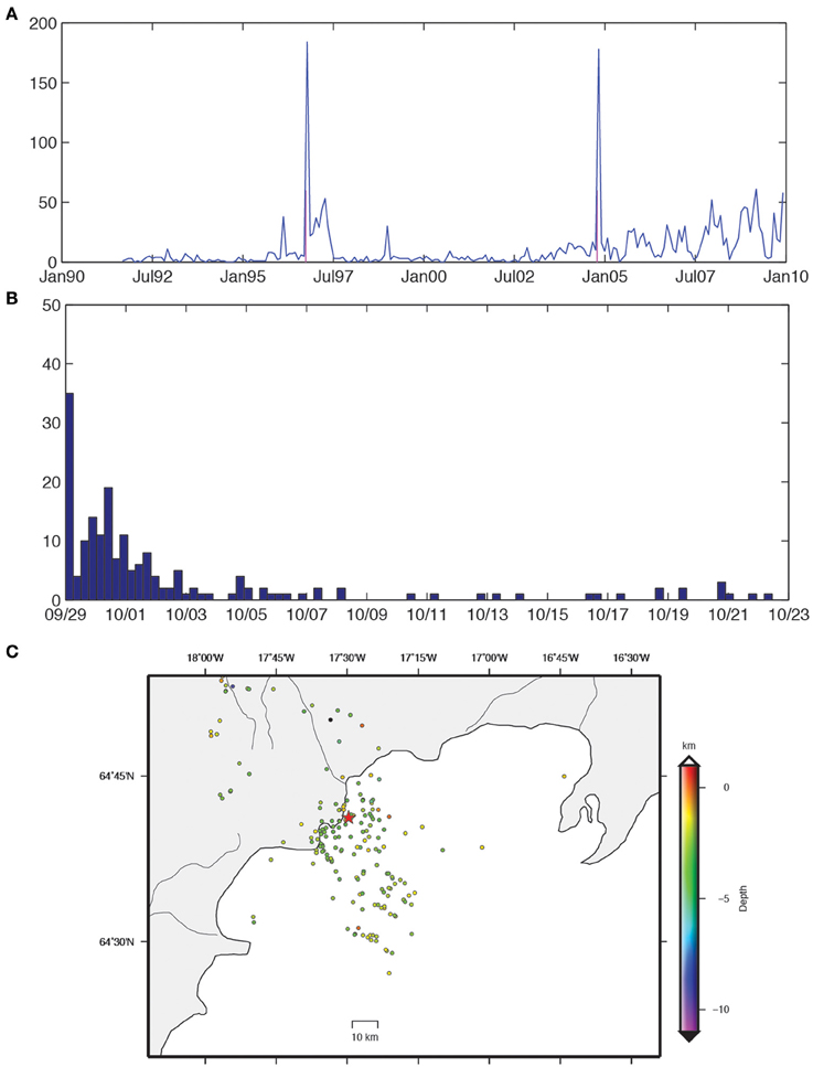
Figure 8. Distribution in time of the seismic events used in this study (see section The Earthquake Catalog Used for Inversion). (A) histogram showing the 20 years span of the database and the two major cluster denoted by the light purple bars based on a time window of 100 earthquakes for 30 days; (B) histogram of the selected cluster for stress analysis of the 1996 Gjálp eruption; (C) distribution of the epicenter of the selected cluster of the eruption 1996 as function of depth in km, red start denotes the main shock occurred the 09/29.

Cluster selected for stress analysis

Prior to the eruption, no particular seismic activity was observed. A significant seismic activity started on the 29th of September 1996 with a main shock of 4.8 moment magnitude (Figures 8B,C). The eruption onset lasted from the 30th of September to the 13th of October and took place on a 6 km long Gjálp fissure (Guðmundsson et al., 2004, Figure 1B), while dyke intrusion is believed to have occurred around the Barðarbunga central volcano (Pagli et al., 2007a). The selected cluster includes 184 earthquakes starting from the main shock on the 29th of September 1996 until the 25th of October 1996 (Figures 8A,C).

Figure 9 shows the general distribution of the strike, dip and rake of the cluster. Two main strike orientations are noted in the range of N095 to N115° and N195 to N210° (Figure 9A). Both nodal planes show dips that can be either relatively gentle (from 45 to 70°) or steep (from 70° to 90°) (Figure 9B). The rake presents two main peaks in the range of −45 to 30° and −170 to 150° (Figure 9C). This cluster denotes a major tendency for strike-slip mechanisms during eruption.

FIGURE 9

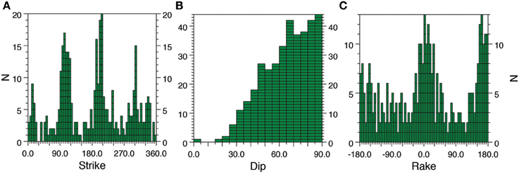
Figure 9. Histograms of the strike (A), dip (B), and rake (C) for both nodal planes of the cluster of the volcanic crisis of 1996 (see section Cluster Selected for Stress Analysis).

Stress analysis

To detail the state of stress, we used another approach to the one that served for the regional stress inversion. A random stress search from the Fsa package (Célérier, 2013, see section Random Stress Search) allowed interactive detection of the mechanically homogenous data subset.

A first stress inversion was applied to the 184 focal mechanisms. It yielded a reduced stress tensor which barely explains all the data. A second stress inversion was run but this time 30% of data were randomly selected and used for inversion to detect different datasets that are mechanically consistent. The resulting solution shows a reduced stress tensor with $\overrightarrow{\sigma }$₃ orientation of N065° associated with a plunge axis of 22° and $\overrightarrow{\sigma }$₁ orientation of N169° associated with a plunge axis of 30° (Φ = 0.8), thus defining a strike-slip regime. This solution explained 78 of the focal mechanisms with an angular α misfit lower than 30°. So this reduced stress tensor was used to reject data that yields an angular α misfit higher than 90°, to obtain a mechanically consistent data subset. Two subsets were thus sorted out, a first one containing 104 focal mechanisms and a second one containing 80 focal mechanisms. From this stage onwards, stress inversions are run on each subset.

Before inverting the data, a P, B, and T-axis analysis for 104 focal mechanisms is performed and presented in Figure 10. Interestingly, the P and T axes have a preferred orientation and the T-axis ranges between N055 and N075° (Figures 10A,B). According to the ternary diagram, most focal solutions are strike-slip in type although reverse and normal ones also occurred. A random stress inversion was applied to this data set. The 10 best reduced stress tensors are retained and these are shown in Figures 10D–H. The orientation of $\overrightarrow{\sigma }$₃ for the best solution is N073° with a plunge of 28° while the orientation of $\overrightarrow{\sigma }$₁ is N333° with a plunge of 17° for a stress shape ratio of 0.72, characterizing a strike-slip regime away from the Andersonian position (Figure 10E). This solution explains 83% of the data (with an angular misfit inferior to 30°, Figure 10G). The average angular misfit of the best solution was 15.9°. As for the regional stress field, an error propagation test was run, showing that the parameters of the reduced stress tensors remain very stable (see section Error Propagation Tests). The 10 best solutions obtained are in agreement with the regional stress field obtained over the 20-year span of this study (Figure 6).

FIGURE 10

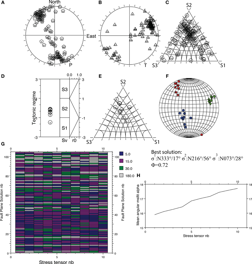
Figure 10. P, B, and T analysis and stress inversion results for the tectonic regime T1. (A) Stereographic projection lower hemisphere of P-axes, (B) Same projection for T-axes, (C) Ternary diagram for the P, B and T axes, S1 = Extension, S2 = Wrench, S3 = Compression (see Figure 3 for references). (D) Tectonic regime plot (Armijo et al., 1982; Philip, 1987; Célérier, 1995) of the 10 best stress tensors resulting from the random stress search. Vertical axis, $\Phi =\left(\frac{{\sigma }_2-{\sigma }_3}{{\sigma }_1-{\sigma }_3}\right)$. (E) Ternary diagram showing the plunge-axes of the 10 best stress tensors. (F) Same projection as for the P and T-axes, red squares denote the orientation of σ₁, blue circles σ₂ and green diamonds σ₃. (G) Table of the best 10 stress tensors in ascending order (x-axis, the first one being the best one), with the individual angular misfit α (between the observed slip and the resolved shear stress) of each datum (y-axis). Blue cases for α > 5°, purple ones for α > 15°, and green ones α > 30°. The gray ones shows α > 30° and then are not explained by the stress tensor. (H) Average misfit α in y-axis for the 10 best stress tensor numbered in x-axis.

As for the first subset, a P, B, and T-axis analysis was performed with the remaining 80 focal mechanisms and the results are presented in Figure 11. A preferred orientation of the T-axis is found; T-axes are mainly orientated in the range of N150–170° (Figures 11A,B). In terms of mechanisms, strike-slip regimes are dominant, although many focal solutions range between reverse and strike-slip positions in the ternary diagrams (Figure 11C). A first stress inversion was performed, yielding an average angular misfit of 20°. This misfit is acceptable, but it is preferable to refine it and run a second stress inversion, to remove the focal solutions with an angular misfit of higher than 90°. The second stress inversion yields an angular misfit of 14°, removing 5 focal solutions. These solutions are satisfactory and very stable, according to the estimation of the 10 best reduced stress tensors. An error propagation test was performed and this confirmed that the reduced stress tensor parameters are stable. Moreover, the best estimated stress tensor explains more than 90% of the data. This stress tensor solution shows a $\overrightarrow{\sigma }$₃ axis of N322° with a stress shape ratio Φ = 0.6 and is characterized by a strike-slip regime away from the Andersonian positions (Figure 11).

FIGURE 11

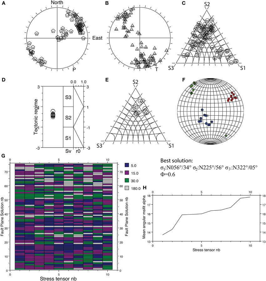
Figure 11. P, B, and T analysis and stress inversion results for the tectonic regime T2. Same legend as Figure 10.

Two states of stress are well-identified: (1) the strike-slip regime with the $\overrightarrow{\sigma }$₃ orientation of N073° (called T1 hereafter), and (2) the strike-slip regime with the $\overrightarrow{\sigma }$₃ orientation of N142° (called T2 hereafter). To illustrate more clearly the difference between the T1 and T2 tectonic regimes, we computed the distance between the 10 best reduced stress tensor solutions of T1 and T2. Lisle and Orife (2002) and Orife and Lisle (2003) defined a measure of the distance between two stress tensors called stress difference, expressed by a single scalar D that takes into account not only the stress orientation but also the stress magnitude (the reader is referred to these references for further details). This parameter D varies from 0 to 2, where 0 means that the two stress tensors are identical and 2 means that they are strictly opposite. The results are shown in Figures 12A,B. It is clear that T1 and T2 are opposite stress tensors since the D values are in the range of 1.8–2. The T1 regime represents 56% of the cluster while the T2 regime represents 41%. 3% (including the main shock) remain unexplained by either T1 or T2.

FIGURE 12

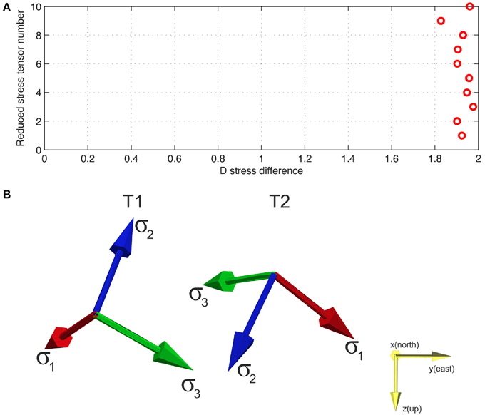
Figure 12. Two opposite reduced stress tensors. (A) Plot of the parameter D (in x-axis) representing a distance between the pair of the 10 best stress tensors solutions of T1 and the best 10 stress tensors of T2 (y-axis, in ascending order where the first one being the best one) that takes into account the stress orientations and the stress shape ratio (see section Stress Analysis, references (Lisle and Orife, 2002; Orife and Lisle, 2003)); (B) 3D perspective of the two opposite stress tensors T1 and T2.

Occurrence of the state of stress and geometrical rotations with time

To observe the occurrence of the T1 and T2 tectonic regimes over time, we simply plotted the focal solutions associated with T1 and T2 as a function of time (Figure 13A). Furthermore, to evaluate rotation of focal mechanisms with time, we consider three-dimensional rotations (3-D) of the geometry of focal mechanisms by an approach such as that described by Kagan (2007). This method considers 3-D rotations by which one double-couple focal mechanism can be turned into another arbitrary focal mechanism. This 3-D rotation is expressed by a single misfit angle noted β. This misfit β angle varies from 0° when the pair of focal mechanisms is identical to a maximum angular misfit of 120°. To calculate β, focal mechanisms need to be compared to an arbitrary frame. We introduced here the frame Q = ($\overrightarrow{p}$, $\overrightarrow{b}$, $\overrightarrow{\tau }$) where $\overrightarrow{p}$, $\overrightarrow{b}$, $\overrightarrow{\tau }$ are unit vectors parallel to the seismological P, B, and T axes respectively (here we used the same frames as Célérier, 2008, 2010). T1 was defined by the frame S_T1 (see section Stress Inversion Principle) and was used to set up an arbitrary frame Q_T1 such that:

$\begin{array}{cc}{S}_{T1}=Q_{T1}& (6)\end{array}$

Yielding a misfit β = 0 between these two frames. Next, each focal mechanism was defined by its frame Q_k (where k = 1, 2, 3…N the number of focal solutions). This was associated with the tectonic regime T1 compared to Q_T1 and the 3D rotation angle β calculated. One should note that Q_T1 (i.e., the arbitrary frame) and Q_k have to be compared in a common reference frame. We use a geographical frame G = ($\overrightarrow{g}$₁; $\overrightarrow{g}$₂; $\overrightarrow{g}$₃) where $\overrightarrow{g}$₁, $\overrightarrow{g}$₂, and $\overrightarrow{g}$₃ are unit vectors pointing north, east and down, respectively. The same process was carried out for T2, where Q_T2 is the second arbitrary frame set up. Rather than the absolute amount of rotation, we considered the relative rotation to qualitatively observe geometrical rotations of the focal solutions over time. This method is simple and has the advantage of not involving stress inversion. The results of the focal solutions with time are presented in Figure 13A. Also, the focal solutions and the rotation β misfit are presented on maps as functions of T1 and T2 (Figure 13B).

FIGURE 13

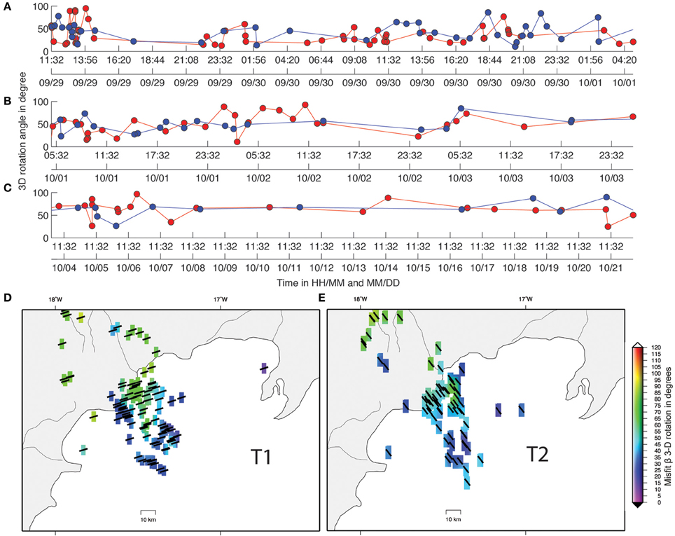
Figure 13. Distribution in time and in space of the tectonic regimes T1 and T2 during the 1996 eruption. (A–C) shows the 3D rotations angle β of each focal solution (Kagan, 2007) compared to the frame Q_T1 for T1 in red and the frame Q_T2 for T2 in blue respectively in y-axis and the time in x-axis, the dots represent the seismic events (see section Occurrence of the State of Stress and Geometrical Rotations with Time). The maps show the amount of 3D rotation β for T1 (D) associated with bars that characterized the location of the seismic events and the orientation of σ_hmin = N073° ± 5° and for T2 (E) with the same features than (D) where the orientation of σ_hmin = N142° ± 7°.

From Figure 13 it is obvious that both tectonic regimes occurred within the same time periods, sometime even within a couple of minutes of each other. Such flip of focal mechanisms over a short time period was seen in the Upptyppingar swarm in 2007 in Iceland, northeast of the glacier (Jakobsdóttir et al., 2008; White et al., 2011). Substantial changes in rotation of focal solutions were mainly observed immediately prior to the eruption (approximately 15 h before its onset) and during the first days of the eruption from 30th of September to 2nd of October). Afterwards, the rotation remains almost standard, but the amount of rotation is relatively greater than during the first days of the eruption. Also, both tectonic regimes occurred spatially in close proximity to each other, so no particular distribution was observed. This feature was also highlighted in the Upptyppingar swarm (Jakobsdóttir et al., 2008; White et al., 2011). However, then the location of the maximum amount of rotation seemed to be located northern of the Barðarbunga volcano where the main shock occurred, and in an ice-free domain (Figure 13B).

Discussion

More than 2400 focal mechanisms spanning a period of almost 20 years (from 1991 to 2009) were inverted to infer a first insight of the regional stress field beneath the Vatnajökull glacier. The contribution of the volcanic, tectonic and isostatic rebound processes will be discussed in the light of recent numerical models to interpret the resulting stress field.

Present-Day State of Stress in the Vatnajökull Region

Regional stress field over a 20 year time-span

The different stress fields obtained by the Hardebeck and Michael (2006) approach revealed a dominance of normal and strike-slip faulting associated with high stress shape ratio (e.i., σ₁ ≈ σ₂). In detail, the ternary diagrams (Figure 5) show rather a continuum between the normal and strike-slip faulting. These features suggest the occurrence of stress permutation between σ₁ and σ₂ in agreement with the stress shape ratio characterizing seismotectonic behavior. Stress permutations between σ₂ and σ₃ also occur but they remain a minor feature. It is well-established that stress permutations such as switching between normal to strike-slip faulting occurred widely throughout Iceland for the present-day stress field (Bergerat et al., 1998; Garcia et al., 2002; Bergerat and Plateaux, 2012) and for paleo-stress fields (Bergerat et al., 1990; Villemin et al., 1994; Guðmundsson et al., 1996; Bergerat and Angelier, 1998; Plateaux et al., 2012). Local conditions such as the uniaxial extension (σ₁ = σ₂ > σ₃), fluid transport and dyking can effectively affect the stress field locally. However, with the database and the method used here the question arises as to whether this permutation reflects oblique mechanisms (i.e., oblique slips) or rather two kinds of pure mechanisms. To answer this question, we selected the cell with the greatest amount of data. One hundred and four focal mechanisms are located around Bárðarbunga volcanoes as shown in Figure 4 at node 15–16 (stress tensor solution n° 48 in Table 1) as a representative cell. We plotted the P, B, and T axes of the 104 focal mechanisms in this cell.

This test does not imply any stress inversion and gives a “direct” observation of the focal mechanisms. The results are presented in Figure 14 and reveal a continuum between normal and strike-slip types. This strongly supports the hypothesis that the stress regime in the studied area is a continuum between normal and strike-slip faulting.

FIGURE 14

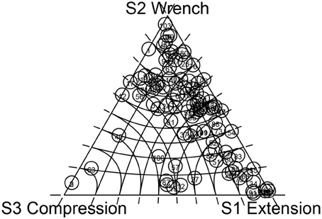
Figure 14. Distribution of the P, B, and T-axes for the 104 focal mechanisms of the cell 15–16 (corresponding to the stress tensor solution number 48, see Table 1).

In terms of stress orientations, two preferred directions of σ_hmin were determined: (1) a direction in agreement with the spreading direction N°105 E according to DeMets et al. (1990, 1994) and (2) a second direction deviated and perpendicular in some places. The damped regional stress field shows that the deviated stress direction is sustained through time mainly around the Bárðarbunga and Grímsvötn central volcanoes while the second direction prevails around the Hamarinn volcano. Interestingly, a gravimetric study of Guðmundsson and Hognadóttir (2007) highlighted that, in contrast to the large central volcanoes such as Grimsvötn and Bárðarbunga, no gravity anomaly is associated with the central volcano of Hamarinn. This volcano is lacking collapse caldera and shares a fissure swarm with the larger volcano of Bárðarbunga. Guðmundsson and Hognadóttir (2007) thus proposed that one of the two central volcanoes within the Veidivötn-Bárðarbunga volcanic system (Figure 1) becomes the dominant one (here the Bárðarbunga) and serves as the main conduit of magma supply, while the Hamarinn is supplied sporadically through sharing-dyke with the dominant one. This might explain why no deviation is observed in the Hamarinn volcano over the period of the study (20 years).

State of stress during the 1996 eruption

The same preferred directions of σ_hmin were determined for the present day stress and the state of stress during the 1996 eruption. However, it appears that the deviated stress direction prevails. Deviated states of stress from both the regional stress field and during the volcanic crisis show similar stress orientations and stress shape ratio (i.e., σ₁ ≈ σ₂).

White et al. (2011) have demonstrated that the flip of normal to reverse focal mechanisms may occur within a minute and in the same location. The two opposite states of stress characterized by the strike-slip regime that were highlighted during the volcanic crisis in 1996 support the same observation of two opposite fracturing mechanisms. Because the two T1 and T2 states of stress show stress regimes distant from the Andersonian positions, P, B, and T axes should be interpreted in terms of fault and slip geometry rather than in terms of stress (Célérier, 2010). White et al. (2011) proposed that the simultaneous normal and reverse sequence mechanisms may be associated with the progressive melt intrusion of a dyke. We propose that during the 1996 eruption, magma intrusion may have caused such sequence as well.

Comparison with other regions

The stress directions described here have been observed elsewhere in Iceland. For instance, a large swarm of earthquakes occurred in 2007 north of the Vatnajökull in the Upptyppingar region at a depth of 14–17 km and it is believed that this was due to dyke intrusion (Jakobsdóttir et al., 2008). Analyses of P, B, and T-axes from fault plane solutions achieved by the Icelandic national survey showed two preferred directions of the T-axis: one is in agreement with the direction of regional spreading and another one lies perpendicular to this (Jakobsdóttir et al., 2008; Plateaux et al., 2012). Interestingly, such an observation has been described for other volcano-tectonic regions such as Mount Etna (Cocina et al., 1996; Patané and Privitera, 2001), Guagua Pichincha in Ecuador (Legrand et al., 2002), the Soufrière Hills volcano (Roman et al., 2008) or Mount St. Helens in Washington (Letho et al., 2010). These studies propose that intruding magma must be the cause of these major changes in the direction of the pressure or tension axes. Thus, we argue that the occurrence of the stress deviations that we observe must be the consequence of volcanic processes prevailing locally on the tectonic ones, not only during a volcanic crisis but also over several years.

Contribution of Numerical Modeling for Stress Interpretation

The contribution of numerical modeling may provide an insight to decipher the “stress signal” of the volcanic, tectonic and isostatic rebound processes from the resulting stress field.

Influence of the glacier retreat

Iceland is currently undergoing glacial isostatic adjustment due to melting of the glaciers (Árnadóttir et al., 2009). Moreover, according to these authors our study area is the fastest rebounding area in Iceland. Therefore, we can expect the regional stress field to be affected by elastic rebound due to glacier thinning. On the base of numerical models of magma transport and isostasic rebound, Hooper et al. (2011), Jull and McKenzie (1996), Maclennan (2002), Sigmundsson et al. (2010a,b), and Pagli and Sigmundsson (2008) showed that decompression due to the recent retreat of the glacier will significantly increase the rate of melt generation in the mantle. However, Sigmundsson et al. (2010a,b) argued that the mode and time scale of transport of the additional magma toward the surface may take longer than decades or centuries. So, we might expect no direct influence of deglaciation on the regional stress field during the short time period of our seismotectonic study (20 years). According to Sigmundsson et al. (2010a,b), the elastic rebound due to the effect of present day ice thinning on the failure of shallow magma chambers should remain small, compared to their natural activity. Therefore, we can discard a notable effect on the expected state of stress (in terms of stress orientation and magnitude) due to the present-day retreat of the glacier, which can be compared to our results.

Stress deviation around volcanoes

A number of studies have attempted to model the stress field in terms of stress orientation and magnitude for volcano-tectonic interactions (Guðmundsson et al., 2005, Guðmundsson and Andrew, 2007). Numerical modeling of Andrew and Guðmundsson (2008) considered for their calculations the magma chambers as elastic inclusions. With these simplifications, they highlighted that a contrast of elastic properties between central volcanoes and their host matrix (e.g., lava pile) may significantly change the stress field. More specifically, the maximum principal stress (σ₁) can change in both magnitude and orientation in the host rocks immediately surrounding the elastic inclusion. These numerical models predict local stress deviation from the spreading direction around volcanoes. Pressurization and depressurization of the magma chamber must also change the stress in direction and in magnitude. Vargas-Bracamontes and Neuberg (2012) propose an interaction between the regional and the magma-induced local stress field, based on the Coulomb failure criterion, to explain the 90° shift of pressure axes (P-axes) referred therein as deviated stress direction from the regional stress field.. According to these authors, when magma pressure starts to increase, the slip (in either a regional or rotated sense of slip relative to the regional maximum compression) also increases. A further increase would tend to promote faulting in the opposite sense from faulting induced by regional stress fields.

Conclusion

While several authors, cited above, stressed the variability of focal mechanisms computed from the records of earthquake swarms, so far no inversion of stress field from focal mechanisms concerning the volcanic regions of Iceland has been published. Therefore, our scientific aim was to study at a small spatial scale the variations of the stress field around and beneath the Vatnajökull ice cap, where no direct observation of faulting is possible.

To do this, we used the methodology developed by Hardebeck and Michael (2006) that allowed us to analyze these variations on a 2.5 × 2.5 km scale during a temporal period of 20 years. To verify the resolution and evaluate the range of errors of our results, we introduced innovative methodologies as propagation test errors, notably the inversion developed by Célérier (2013). We also computed the stress difference as proposed by Lisle and Orife (2002) to extract distinct tectonic regimes.

In this paper, we describe the characterization of a continuum between strike-slip and extensive faulting with a high stress shape ratio Φ. We highlight local permutations between σ₁ and σ₂ and horizontal deviations of the stress pattern. Two main directions of σ_hmin were revealed: one in agreement with the regional spreading and second deviated, and even perpendicular to the first in some places. The deviated stress direction is sustained through the 20 year span of the study around the Bárðarbunga and Grimsvötn central volcanoes while the spreading direction remains predominant around the Hamarinn volcano. This result supports the hypothesis that this volcano lacks collapse caldera and shares a fissure swarm with the larger Bárðarbunga volcano.

During the 1996 eruption, two opposite strike-slip stress regimes occur: one in agreement with the spreading direction and the other deviated from this direction, which prevails during the volcanic crisis. Because these two states of stress T1 and T2 show stress regimes away from the Andersonian positions, P, B, and T axes, the rapid flip between these two regimes may be associated with the progressive melt intrusion of a dyke.

As a whole, the detailed study of stress regimes in this volcanic region provides not only a description of P, B, and T axis direction, but also allows the fracturing mechanisms over the long-term and during an intrusion/eruption sequence to be inferred through determination of the stress shape ratio Φ. Such stress deviations and/or permutations may favor the reactivation of faults and could explain the intense seismicity observed in the Vatnajökull region. Because such stress perturbations have already been noticed in other volcano-tectonic regions, such a detailed procedure of studying stress regimes at several spatial and temporal scales could be applied to other volcanic regions.

Conflict of Interest Statement

The authors declare that the research was conducted in the absence of any commercial or financial relationships that could be construed as a potential conflict of interest.

Acknowledgments

We thank Bergþóra S. Þorbjarnardóttir for help in providing the earthquakes catalog from IMO. We are also grateful to Bernard Célérier for fruitful discussions. Thanks to Marie Keiding for providing comments on the manuscript. We also would like to thank the editor Valerio Acocella and three anonymous reviewers for improving the manuscript. SATSI code (Spatial And Temporal Stress Inversion) was used for inverting data and was downloaded from USGS website (http://earthquake.usgs.gov/research/software/). Figures were made using GMT, MATLAB and ParaView.

References

Aki, K., and Richards, P. G. (1980). Quantitative Seismology: Theory and Methods. San Francisco, CA: W.H. Freeman.

Allen, R. M., Nolet, G., Morgan, W., Vogfjord, K., Nettles, M., Ekstrom, G., et al. (2002). Plume-driven plumbing and crustal formation in Iceland. J. Geophys. Res. 107, 1–19. doi: 10.1029/6202001JB000584

CrossRef Full Text

Andrew, R., and Guðmundsson, Á. (2008). Volcanoes as elastic inclusions: their effects on the propagation of dykes, volcanic fissures, and volcanic zones in Iceland. J. Volcanol. Geotherm. Res. 177, 1045–1054. doi: 10.1016/j.jvolgeores.2008.07.025

CrossRef Full Text

Angelier, J. (1975). Sur l'analyse de mesures recueillies dans des sites faillés: l'utilité d'une confrontation entre les méthodes dynamiques et cinématiques. C. R. Acad. Sci. D281, 1805–1808.

Angelier, J. (1979). Determination of the mean principal directions of stresses for a given fault population. Tectonophysics 56, T17–T26. doi: 10.1016/0040-1951(79)90081-7

CrossRef Full Text

Angelier, J. (1984). Tectonic analysis of fault slip data sets. J. Geophys. Res. 89, 5835–630 5848.

Angelier, J. (2002). Inversion of earthquake focal mechanisms to obtain the seismotectonic stress-IV. A new method free of choice among nodal planes. Geophys. J. Int. 150, 588–609. doi: 10.1046/j.1365-246X.2002.01713.x

CrossRef Full Text

Angelier, J., and Manoussis, S. (1980). Classification automatique et distinction des phases superposées en tectonique de failles. C. R. Acad. Sci. D 290, 651–654

Armijo, R., Carey, E., and Cisternas, A. (1982). The inverse problem in microtectonics and the separation of tectonic phases. Tectonophysics 82, 145–160. doi: 10.1016/0040-1951(82)90092-0

CrossRef Full Text

Armijo, R., and Cisternas, A. (1978). Un problème inverse en microtectonique cassante. C. R. Acad. Sci. 638D, 595–598

Árnadóttir, T., Lund, B., Jiang, W., Geirsson, H., Björsson, H., and Einarsson, P. (2009). Glacial rebound and plate spreading: results from the first countrywide GPS observations in Iceland. Geophys. J. Int. 177, 691–716. doi: 10.1111/j.1365-246X.2008.04059.x

CrossRef Full Text

Bergerat, F. (1987). Stress fields in the European platform at the time of Africa-Eurasia collision. Tectonics 6, 99–132. doi: 10.1029/TC006i002p00099

CrossRef Full Text

Bergerat, F., and Angelier, J. (1998). Fault systems and paleostresses in the Vestfirdir Peninsula. Relationships with the tertiary paleo-rifts of Skagi and Snaefells. Geodinamica Acta. 11, 105–118. doi: 10.1016/S0985-3111(98)80008-9

CrossRef Full Text

Bergerat, F., Angelier, J., and Villemin, T. (1990). Fault systems and stress patterns on emerged oceanic ridges: a case study in Iceland. Tectonophysics 179, 183–197. doi: 10.1016/0040-1951(90)90290-O

CrossRef Full Text

Bergerat, F., Guðmundsson, Á., Angelier, J., and Rögnvaldsson, S. T. (1998). Seismotectonics of the central part of the South Iceland Seismic Zone. Tectonophysics 298, 319–335. doi: 10.1016/650S0040-1951(98)00191-7

CrossRef Full Text

Bergerat, F., and Plateaux, R. (2012). Architecture and development of (Pliocene to Holocene) faults and fissures in the East Volcanic Zone of Iceland. C. R. Géosci. 344, 191–204. doi: 10.1016/653j.crte.2011.12.005

CrossRef Full Text

Bjórnsson, H., Björn, S., and Sigurgeirsson, T. (1982). Penetration of water into hot rock boundaries of magma at Grímsvötn. Nature 295, 580–581. doi: 10.1038/295580a0

CrossRef Full Text

Bjórnsson, H., Pálsson, F., and Guðmundsson, M. T. (1992). Vatnajökull, Northwestern Part. 1:100 000. Bedrock Map. Landsvirkjun og Raunvísindastofnun Háskólans.

Böðvarsson, R., Rögnvaldsson, S. T., Jakobsdóttir, S. S., Slunga, R., and Stefansson, R. (1996). The SIL data acquisition and monitoring system. Seismol. Res. Lett. 67, 35–46. doi: 10.1785/gssrl.67.5.35

CrossRef Full Text

Bott, M. H. (1959). The mechanisms of oblique slip faulting. Geol. Mag. 96, 109–117. doi: 10.1017/S0016756800059987

CrossRef Full Text

Burg, J., Célérier, B., Chaudhry, N. M., Ghazanfar, M., Gnehm, F., and Schnellmann, M. (2005). Fault analysis and paleostress evolution in large strain regions: methological and geological discussion of the southeastern Himalayan fold-and-thrust belt in Pakistan. J. Asian Earth Sci. 24, 445–467. doi: 10.1016/j.jseaes.2003.12.008

CrossRef Full Text

Célérier, B. (1995). Tectonic regime and slip orientation of reactivated faults. Geophys. J. Int. 121, 143–161. doi: 10.1111/j.1365-246X.1995.tb03517.x

CrossRef Full Text

Célérier, B. (2008). Seeking Anderson's faulting in seismicity: a centennial celebration. Rev. Geophys. 46, 1–34. doi: 10.1029/2007RG000240

CrossRef Full Text

Célérier, B. (2010). Remarks on the relationship between the tectonic regime, the rake of the slip vectors, the dip of the nodal planes, and the plunges of the P, B, and T axes of earthquake focal mechanisms. Tectonophysics 482, 42–49. doi: 10.1016/j.tecto.2009.03.006

CrossRef Full Text

Célérier, B. (2013). FSA Version 35.1: Fault and Stress Analysis Software. Available online at: http://www.pages-perso-bernard-celerier-univ-montp2.fr/software/dcmt/fsa/fsa.html

Célérier, B., Etchecopar, A., Bergerat, F., Vergely, P., Arthaud, F., and Laurent, P. (2012). Inferring stress from faulting: from early concepts to inverse methods. Tectonophysics 581, 206–219. doi: 10.1016/j.tecto.6752012.02.009

CrossRef Full Text

Cocina, O., Neri, G., and Privitera, S. (1996). Earthquake and stress tensor space-time distribution at Mount Etna before the 1991–1993 volcanic eruption. Acta Vulcanol. 8, 15–22

Darbyshire, F. A., Bjarnason, I. T., White, R. S., and Flovenz, O. G. (1998). Crustal structure above the Iceland mantle plume imaged by the ICEMELT refraction profile. Geophys. J. Int. 680, 1131–1149. doi: 10.1046/j.1365-246X.1998.00701.x

CrossRef Full Text

Darbyshire, F. A., White, R. S., and Priestley, K. F. (2000). Structure of the crust and uppermost mantle of Iceland from a combined seismic and gravity study. Earth Planet. Sci. Lett. 181, 409–428. doi: 10.1016/S0012-821X(00)00206-5

CrossRef Full Text

Delvaux, D., and Sperner, B. (2003). New aspects of tectonic stress inversion with reference to the tensor program. Geol. Soc. Lond. Spec. Publ. 212, 75–100. doi: 10.1144/GSL.SP.2003.212.01.06

CrossRef Full Text

DeMets, C., Gordon, R. G., Argus, F., and Stein, S. (1990). Current plate motions. Geophys. J. Int. 101, 425–478. doi: 10.1111/j.1365-246X.1990.tb06579.x

CrossRef Full Text

DeMets, C., Gordon, R. G., Argus, F., and Stein, S. (1994). Effect of recent revisions to the geomagnetic reversal time scale on estimates of current plate motion. Geophys. Res. Lett. 21, 2191–2194. doi: 10.1029/94GL02118

CrossRef Full Text

Einarsson, P. (1991). Earthquakes and present-day tectonism in Iceland. Tectonophysics 189, 261–279. doi: 10.1016/0040-1951(91)90501-I

CrossRef Full Text

Etchecopar, A. (1984). Étude des états de contrainte en tectonique cassante et simulations de déformations plastiques (approche mathématique). Thèse d'État ès Sciences, Université des Sciences et Techniques du Languedoc, 269.

Etchecopar, A., Vasseur, G., and Daignieres, M. (1981). An inverse problem in microtectonics for the determination of stress tensors from fault striation analysis. J. Struct. Geol. 3, 51–65. doi: 10.1016/0191-8141(81)90056-0

CrossRef Full Text

Frohlich, C. (1992). Triangle diagrams: ternary graphs to display similarity and diversity of earthquake focal mechanisms. Phys. Earth Planet. Interiors 75, 193–198. doi: 10.1016/0031-9201(92)90130-N

CrossRef Full Text

Garcia, S., Angelier, J., Bergerat, F., and Homberg, C. (2002). Tectonic analysis of an oceanic transform fault zone based on fault-slip data and earthquake focal mechanisms: the Húsavík–Flatey Fault zone, Iceland. Tectonophysics 344, 157–174. doi: 10.1016/S0040-1951(01)00282-7

CrossRef Full Text

Gephart, J. W. (1985). Principal stress directions and the ambiguity in fault plane identification from focal mechanisms. Bull. Seismol. Soc. Am. 75, 621–625

Guðmundsson, Á., Acocella, V., and Denatale, G. (2005). The tectonics and physics of volcanoes. J. Volcanol. Geotherm. Res. 144, 1–5. doi: 10.1016/j.jvolgeores.2004.12.002

CrossRef Full Text

Guðmundsson, Á., and Andrew, R. E. B. (2007). Mechanical interaction between active volcanoes in Iceland. Geophys. Res. Lett. 34, 1–5. doi: 10.1029/2007GL029873

CrossRef Full Text

Guðmundsson, Á., Bergerat, F., and Angelier, J. (1996). Off-rift and rift-zone palaeostresses in Northwest Iceland. Tectonophysics 255, 211–228. doi: 10.1016/0040-1951(95)00138-7

CrossRef Full Text

Guðmundsson, M., Sigmundsson, F., Bjórnsson, H., and Hognadóttir, T. (2004). The 1996 eruption at Gjalp, Vatnajakull ice cap, Iceland: efficiency of heat transfer, ice deformation and subglacial water pressure. Bull. Volcanol. 66, 46–65. doi: 10.1007/s00445-003-0295-9

CrossRef Full Text

Guðmundsson, M. T., and Hognadóttir, T. (2007). Volcanic systems and calderas in the Vatnajökull region, central Iceland: constraints on crustal structure from gravity data. J. Geodyn. 43, 153–169. doi: 10.1016/j.jog.2006.09.015

CrossRef Full Text

Hardebeck, J. L., and Michael, A. J. (2006). Damped regional-scale stress inversions: methodology and examples for southern California and the Coalinga aftershock sequence. J. Geophys. Res. 722, 1–11. doi: 10.1029/2005JB004144

CrossRef Full Text

Hooper, A., Ófeigsson, B. G., Sigmundsson, F., Lund, B., Einarsson, P., Geirsson, H., et al. (2011). Increased capture of magma in the crust promoted by ice-cap retreat in Iceland. Nat. Geosci. 4, 783–786. doi: 10.1038/ngeo1269

CrossRef Full Text

Jakobsdóttir, S. S., Roberts, M. J., Guðmundsson, G. B., Geirsson, H., and Slunga, R. (2008). Earthquake swarms at Upptyppingar, north-east Iceland: a sign of magma intrusion? Stud. Geophys. Geodaetica 52, 513–528. doi: 10.1007/s11200-008-0035-x

CrossRef Full Text

Jóhannesson, H., and Sæmundsson, K. (1998). “Geological map of Iceland, 1:500000. Bedrock Geology,” in Icelandic Institute of Natural History and Iceland Geodetic Survey (Reykjavik).

Jull, M., and McKenzie, D. P. (1996). The effect of deglaciation on mantle melting. J. Geophys. Res. 101, 21815–21828. doi: 10.1029/96JB01308

CrossRef Full Text

Kagan, Y. Y. (2007). Simplified algorithms for calculating double-couple rotation. Geophys. J. Int. 171, 411–418. doi: 10.1111/j.1365-246X.2007.03538.x

CrossRef Full Text

Larsen, G. (2002). “A brief overview of eruptions from ice-covered and ice-capped volcanic system in Iceland during the last 11 centuries: frequency, periodicity and implications,” in Ice-volcano Interaction on Earth and Mars, Vol. 202, eds J. L. Smellie and M. G. Chapman (London: Geological Society), 81–90. doi: 10.1144/GSL.SP.2002.202.01.05

CrossRef Full Text

Larsen, G., Guðmundsson, M. T., and Björnsson, H. (1998). Eight centuries of periodic volcanism at the center of the Iceland hotspot revealed by glacier tephrostratigraphy. Geology 26, 943. doi: 10.1130/7450091-7613(1998)026<0943:ECOPVA>2.3.CO;2

CrossRef Full Text

Legrand, D., Calahorrano, A., Guillier, B., Rivera, L., Ruiz, M., Villagomez, D., et al. (2002). Stress tensor analysis of the 1998–1999 tectonic swarm of northern Quito related to the volcanic swarm of Guagua Pichincha Volcano, Ecuador. Tectonophysics 344, 15–36. doi: 10.1016/S0040-1951(01)00273-6

CrossRef Full Text

Letho, H. L., Roman, D. C., and Moran, S. C. (2010). Temporal changes in stress preceding the 2004-2008 eruption of Mount St. Helens, Washington. J. Volcanol. Geotherm. Res. 751, 129–142. doi: 10.1016/j.jvolgeores.2010.08.015

CrossRef Full Text

Liesa, C., and Lisle, R. J. (2004). Reliability of methods to separate stress tensors from heterogeneous fault-slip data. J. Struct. Geol. 26, 559–572. doi: 10.1016/j.jsg.2003.08.010

CrossRef Full Text

Lisle, R. J., and Orife, T. (2002). STRESSTAT: a Basic program for numerical evaluation of multiple stress inversion results. Comput. Geosci. 28, 1037–1040. doi: 10.1016/S0098-3004(02)00018-3

CrossRef Full Text

Lisle, R. J., and Vandycke, S. (1996). Separation of multiple stress events by fault striation analysis: an example from Variscan and younger structures at Ogmore, SouthWales. J. Geol. Soc. 153, 945.

Lund, B., and Townend, J. (2007). Calculating horizontal stress orientations with full or partial knowledge of the tectonic stress tensor. Geophys. J. Int. 170, 1328–1335. doi: 10.1111/j.1365-246X.2007.03468.x

CrossRef Full Text

Maclennan, J. (2002). The link between volcanism and deglaciation in Iceland. Geochem. Geophys. Geosyst. 3, 1062. doi: 10.1029/2001GC000282

CrossRef Full Text

Mercier, J., and Carey-Gailhardis, E. (1989). Regional state of stress and characteristic fault kinematics instabilites shown by aftershock sequences: the aftershock sequences of the 1978 Thessalonki (Greece) and 1980 Campania-Lucania (italia) earthquakes as examples. Earth Planet. Sci. Lett. 92, 247–264. doi: 10.1016/0012-821X(89)90050-2

CrossRef Full Text

Michael, A. J. (1984). Determination of stress from slip data: faults and folds. J. Geophys. Res. 89, 11517–11526. doi: 10.1029/JB089iB13p11517

CrossRef Full Text

Michael, A. J. (1987). Use of focal mechanisms to determine stress: a control study. J. Geophys. Res. 92, 357–368. doi: 10.1029/JB092iB01p00357

CrossRef Full Text

Orife, T., and Lisle, R. J. (2003). Numerical processing of paleostress results. J. Struct. Geol. 25, 949–957. doi: 10.1016/S0191-8141(02)00120-7

CrossRef Full Text

Pagli, C., and Sigmundsson, F. (2008). Will present day glacier retreat increase volcanic activity? Stress induced by recent glacier retreat and its effect on magmatism at the Vatnajökull ice cap, Iceland. Geophys. Res. Lett. 35, 3–7. doi: 10.1029/2008GL033510

CrossRef Full Text

Pagli, C., Sigmundsson, F., Lund, B., Sturkell, E., Geirsson, H., Einarsson, P., et al. (2007a). Glacioisostasic deformation around the Vatnajökull ice cap, Iceland, induced by recent climate warming: GPS observations and finite element modeling. J. Geophys. Res. 112, 97–108. doi: 10.1029/2006JB004421

CrossRef Full Text

Patané, D., and Privitera, S. (2001). Seismicity related to 1989 and 1991-93 Mt. Etna Italy eruptions: kinematic constraints by fault plane solution analysis. J. Volcanol. Geotherm. Res. 787, 77–98. doi: 10.1016/S0377-0273(00)00305-X

CrossRef Full Text

Philip, H. A. (1987). Plio-Quaternary evolution of the stress field in Mediterranean zones of subduction and Collision. Anna. Geophys. 5B, 301–320.

Plateaux, R., Bergerat, F., Béthoux, N., Villemin, T., and Gerbault, M. (2012). Implications of fracturing mechanisms and fluid pressure on earthquakes and fault slip data in the east Iceland rift zone. Tectonophysics 581, 19–34. doi: 10.1016/j.tecto.2012.01.013

CrossRef Full Text

Rögnvaldsson, S. T., and Slunga, R. (1993). Routine fault plane solutions for local networks: a test with synthetic data. Bull. Seismol. Soc. Am. 11, 1232–1247.

Rögnvaldsson, S. T., and Slunga, R. (1994). Single and joint fault plane solutions for microearthquakes in South Iceland. Tectonophysics 237, 73–86. doi: 10.1016/0040-1951(94)90159-7

CrossRef Full Text

Roman, D., De Angelis, S., Latchman, J., and White, R. (2008). Patterns of volcanotectonic seismicity and stress during the ongoing eruption of the Soufrière Hills Volcano, Montserrat (1995–2007). J. Volcanol. Geotherm. Res. 173, 230–244. doi: 10.1016/j.jvolgeores.2008.01.014

CrossRef Full Text

Sæmundsson, K. (1979). Outline of the geology of Iceland. Jokull 29, 7–28.

Sigmundsson, F., and Guðmundsson, M. (2004). The Grímsvötn eruption, november 2004. in Icelandic. Jokull 54, 139–142.

Sigmundsson, F., Hreinsdóttir, S., Hooper, A., Árnadóttir, T., Pedersen, R., Roberts, M. J., et al. (2010a). Intrusion triggering of the 2010 Eyjafjallajökull explosive eruption. Nature 468, 426–430. doi: 10.1038/nature09558

Pubmed Abstract | Pubmed Full Text | CrossRef Full Text

Sigmundsson, F., Pinel, V., Lund, L., B, Albino, F., Pagli, C., Geirsson, H., et al. (2010b). Climate effects on volcanism: influence on magmatic systems of loading and unloading from ice mass variations, with examples from Iceland. Philos. Trans. R. Soc. 368, 2519–2534. doi: 10.1098/809rsta.2010.0042

Pubmed Abstract | Pubmed Full Text | CrossRef Full Text

Sperner, B., and Zweigel, P. (2010). A plea for more caution in fault-slip analysis. Tectonophysics 482, 29–41. doi: 10.1016/j.tecto.2009.07.019

CrossRef Full Text

Thordarson, T., and Larsen, G. (2007). Volcanism in Iceland in historical time: Volcano types, eruption styles and eruptive history. J. Geodyn. 43, 118–152. doi: 10.1016/j.jog.2006.09.005

CrossRef Full Text

Tryggvason, K., Husebye, E. S., and Stefansson, R. (1983). Seismic image of the hypothesized icelandic hot spot. Tectonophysics 100, 97–188. doi: 10.1016/0040-1951(83)90180-4

CrossRef Full Text

Vargas-Bracamontes, D. M., and Neuberg, J. W. (2012). Interaction between regional and magma-induced stresses and their impact on the volcano-tectonic seismicity. J. Volcanol. Geotherm. Res. 243–244, 91–96. doi: 10.1016/j.jvolgeores.2012.06.025

CrossRef Full Text

Villemin, T., Bergerat, F., Angelier, J., and Lacasse, C. (1994). Brittle deformation and fracture patterns on oceanic rift shoulders : the Esja peninsula, SW Iceland. J. Struct. Geol. 16, 1654–1994. doi: 10.1016/0191-8141(94)90132-5

CrossRef Full Text

Wallace, R. E. (1951). Geometry of shearing stress and relation to faulting. J. Geol. 59, 118–130. doi: 10.1086/625831

CrossRef Full Text

White, R. S., Drew, J., Martens, H. R., Key, J., Soosalu, H., and Jakobsdóttir, S. S. (2011). Dynamics of dyke intrusion in the mid-crust of Iceland. Earth Planet. Sci. Lett. 304, 300–312. doi: 10.1016/j.epsl.2011.02.038

CrossRef Full Text

Yamaji, A. (2000). The multiple inverse method: a new technique to separate stresses from heterogeneous fault-slip data. J. Struct. Geol. 22, 441–452. doi: 10.1016/S0191-8141(99)00163-7

CrossRef Full Text

Yamaji, A. (2003). Are the solutions of stress inversion correct? Visualization of their reliability and the separation of stresses from heterogeneous fault-slip data. J. Struct. Geol. 25, 241–252. doi: 10.1016/S0191-8141(02)00021-4

CrossRef Full Text