Observational study of land-surface-cloud-atmosphere coupling on daily timescales

Introduction

Analysis of the long-term Canadian Prairie data set is transforming our understanding of land-atmosphere coupling and more broadly hydrometeorology (Betts et al., 2014a). From the early 1950s to the present, these data contain a remarkable set of hourly observations of opaque or reflective cloud cover in tenths, made by trained observers who have followed the same protocol for 60 years (MANOBS, 2013). Betts et al. (2013) calibrated these opaque cloud observations against multiyear shortwave and longwave radiation data to quantify the impact of clouds. This gives the so-called shortwave and longwave cloud forcing (SWCF, LWCF), as well as net radiation, R_n. Many climate studies have been limited to temperature and precipitation for which long-term records are generally available. Similarly, model climate change analyses typically focus on temperature and precipitation, and it is thought that uncertainties in cloud processes explain much of the spread in modeled climate sensitivity (Flato et al., 2013). In contrast, the Canadian Prairie data have 60 years of hourly records for the fully coupled system of temperature, relative humidity (RH), precipitation, and radiation derived from cloud observations. The diurnal cycle is tightly coupled to clouds and radiation (Betts et al., 2013), but on monthly timescales, temperature and RH are jointly coupled to precipitation, cloud cover and radiation (Betts et al., 2014a). They found that up to 60–80% of the monthly variance in the diurnal temperature range, afternoon RH and lifting condensation level could be explained in terms of monthly anomalies of opaque cloud and precipitation. From this it is clear that four variables, temperature, RH, radiation and precipitation are all essential for understanding hydrometeorology and hydroclimatology.

The role of clouds and radiative forcing has been missing in much of the literature on land-atmosphere coupling, where the focus has been largely on surface variables, such as soil moisture and albedo (Koster and Suarez, 2001; Koster et al., 2004; Dirmeyer, 2006; Ferguson and Wood, 2011; Ferguson et al., 2012; Koster and Manahama, 2012; Santanello et al., 2013) following earlier work by Betts and Ball (1995, 1998), Beljaars et al. (1996) and Eltahir (1998). The framework for describing atmospheric controls on soil moisture–boundary layer interactions (Findell and Eltahir, 2003) used two lower-atmosphere metrics: the convective triggering potential and low-level humidity, but not the clouds that are part of the tightly coupled boundary layer system. Modeling studies of course highlight the critical role of the cloud and radiation fields on land-surface processes (e.g., Betts, 2004; Betts and Viterbo, 2005; Betts, 2007), but the wide variation between models (Dirmeyer et al., 2006; Guo et al., 2006; Koster et al., 2006; Taylor et al., 2013) may reflect in part model errors in the cloud fields. However, while there has been ongoing work to benchmark uncoupled land surface models (Abramowitz, 2012), there are still a lack of appropriate metrics for benchmarking coupled land-atmosphere models. Using the 600 station-years of data from the Canadian Prairies, we can finally begin to develop coupled benchmarking metrics and relationships necessary to test model behavior against observations.

Betts et al. (2013) showed that there is marked difference between a warm season state with an unstable daytime convective boundary layer (BL), controlled by the SWCF, and a cold season state with surface snow with a stable BL, controlled by the LWCF. Betts et al. (2014b) looked at the rapid transitions that occur with snow cover between the warm season convective BL and the cold season stable BL. This paper will revisit with much greater precision the calibration of the opaque cloud data, for the warm and cold seasons, using 17 years of data from the baseline surface radiation network (BSRN) site at Bratt's Lake in Saskatchewan, and co-located grid-point data from the European Center reanalysis known as ERA-Interim. Then we shall examine in more detail the physical processes influencing land-atmosphere coupling and the daily climate in the warm season. The daily timescale analysis framework that we use here was proposed by Betts (2004), and applied in several studies using model data from reanalysis (Betts and Viterbo, 2005; Betts, 2006, 2009) and to compare reanalysis and observations over the boreal forest (Betts et al., 2006). It has proved useful for other recent studies of land-atmosphere coupling (Ferguson et al., 2012; Dirmeyer et al., 2014).

Our intent is to provide an observational reference for the evaluation of both simplified models, and the large-scale models we depend upon for weather forecasting and climate simulation, where most land-surface-BL and cloud processes have to be parameterized. From an analysis perspective, the key addition is having a quantitative estimate of the surface radiation as well as the traditional surface climate variables. In Section Data and Analysis Methods we outline our analysis framework. In Section Analysis of the BSRN Data, we first analyze the BSRN and ERA-Interim data to look at the annual cycle of the SWCF and LWCF. We show the warm season coupling between SW and LW radiation and the diurnal ranges of temperature and RH at the BSRN site. Then we calibrate the opaque cloud data at Regina in Saskatchewan against the nearby BSRN data for the cold and warm seasons. In Section Dependence of Daily Climate in Summer on Opaque Cloud and other Variables, we merge the 11 Prairie stations to give us about 600 station-years of data, and map how different physical processes affect daily land-surface climate in summer, June, July and August (JJA). Specifically, after stratifying by opaque cloud, we will identify the daily climate signature of wind, relative humidity, the day-night asymmetry of the cloud field, and monthly weighted precipitation anomalies. In Section Dependence of Summer Climate on ECA and LW_n we remap the diurnal climate signatures in terms of surface net longwave and effective cloud albedo, and Section Summary and Conclusions summarizes our conclusions.

Data and Analysis Methods

Climate Variables and Data Processing

We analyzed data from the 11 climate stations listed in Table 1: the stations are all at airports across the Canadian Prairies. They have hourly data, starting in 1953 for all stations, except Regina and Moose Jaw which start in 1954. The last year with complete precipitation data (that was available in 2012 when these data were processed) is listed after the station name.

TABLE 1

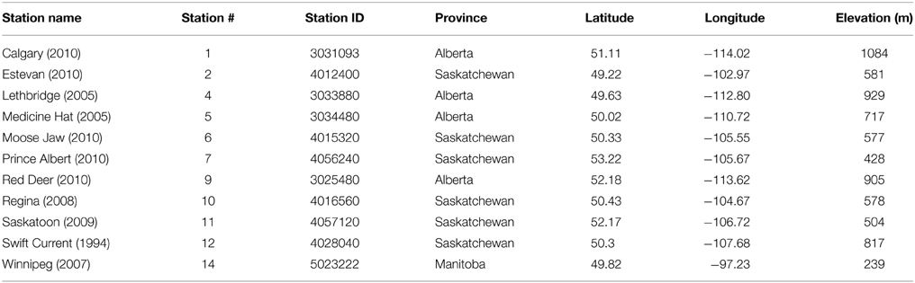
Table 1. Climate stations: location and elevation.

The hourly climate variables include surface pressure (p), dry bulb temperature (T), relative humidity (RH), windspeed and direction, total opaque cloud amount and total cloud amount. The time-base is Local Standard Time (LST). Trained observers have followed the same cloud observation protocol for 60 years (MANOBS, 2013). Opaque (or reflective) cloud is defined (in tenths) as cloud that obscures the sun, or the moon and stars at night. The long-term consistency of these hourly opaque cloud fraction observations makes them useful for climate studies. Betts et al. (2013) used four stations, Lethbridge, Swift Current, Winnipeg and The Pas (in the boreal forest), with downward shortwave radiation SW_dn to calibrate the daily mean total opaque cloud fraction, OPAQ_m, in terms of daily SWCF. They also used downward longwave radiation LW_dn from Saskatoon and Prince Albert National Park for the calibration of OPAQ_m to net longwave (LW_n) on daily timescales. Here we extend these analyses using the BSRN data, which is 25 km from the Regina climate station.

We generated a file of daily means for all variables, such as mean temperature and humidity, T_m and RH_m, and extracted and appended to each daily record the corresponding hourly data at the times of maximum and minimum temperature (T_x and T_n). We merged a file of daily total precipitation (and daily snow depth, not used here). Since occasional hourly data were missing, we kept a count of the number of measurement hours, MeasHr, of valid data in the daily mean. In our results here we have filtered out all days for which MeasHr <20. However, with almost no missing hours of data in the first four decades, there are very few missing analysis days, except for Swift Current, where night-time data is missing from June 1980 to May 1986, and Moose Jaw, where night-time measurements ceased after 1997.

From the hourly data we compute the diurnal temperature range between maximum temperature, T_x, and minimum temperature, T_n, as:

$\begin{array}{cc}\text{DTR}={\text{T}}_{\text{x}}-{\text{T}}_{\text{n}}& \left(1\right)\end{array}$

We also define the difference of relative humidity, RH, between T_n and T_x, as:

$\begin{array}{cc}\Delta \text{RH}={\text{RH}}_{\text{x}}-{\text{RH}}_{\text{n}}\approx {\text{RH}}_{\text{tn}}-{\text{RH}}_{\text{tx}}& \left(2\right)\end{array}$

Where RH_x, RH_n are the maximum and minimum RH. This approximation is excellent in the warm season, when surface heating couples with a convective BL. Then typically RH reaches a maximum near sunrise at T_n and a minimum at the time of the afternoon T_x (Betts et al., 2013). We also derived from p, T_x and RH_tx, the lifting condensation level (LCL), the pressure height to the LCL, P_LCLtx, mixing ratio (Q_tx) and equivalent potential temperature, θ_Etx, all at the time of the maximum temperature. Similarly we derived Q_tn, θ_Etn, and P_LCLtn at the time of the minimum temperature, T_n.

This Prairie data set is large and includes the synoptic variability for nearly 600 station-years. For summer (JJA) there are about 54,000 days with good data. We will bin the data and generate means for many sub-stratifications, to isolate the climatological coupling between different variables in this fully coupled system. As an estimate of the uncertainty in a mean value, derived from N daily values, we will show the standard error (SE) of the mean, calculated from the standard deviation (SD) as SE = SD/√N. As a result, larger SE values generally indicate a smaller data sample N. For the larger dataset we will not show a mean value unless N > 200, and for the much smaller BSRN dataset, we reduced this threshold to N = 40. Many plots with a 2-way stratification (e.g., showing the dependence of DTR on opaque cloud and windspeed) may have >500 days in each bin, so the SE of each point is small. We will also use multiple linear regression of the daily data to assess the scatter in quasi-linear relationships.

BSRN data

Canada's BSRN station was a Prairie site at Bratt's Lake, Saskatchewan at 50.204°N, 104.713°W at an elevation of 588 m. We will use it to calibrate the opaque clouds observed at Regina, about 25 km to the north in terms of SWCF and net longwave flux (LW_n). We processed the raw 1-min mean BSRN data to hourly means (with standard deviation, max and min) for the 17-year period of 1995–2011. We filtered the long-wave down (LW_dn) data, removing from the hourly average extreme values greater than 3 standard deviations of the 1-min data for each month. The data quality is high for the first 14 years, and this LW filtering removed less than 0.5% of the 1-min data values. During July–October, 2009 and June–August, 2010, the long-wave data appears to have a bias of unknown origin and these data were not used. For shortwave down (SW_dn), we removed hourly values at night < ±1 W/m². The dataset includes temperature and pressure for all years, and relative humidity for 2000–2011.

We have no measurements of the upward components (SW_up and LW_up). Defining a surface albedo, α_s, gives the net shortwave:

$\begin{array}{cc}{\text{SW}}_{\text{n}}={\text{SW}}_{\text{dn}}-{\text{SW}}_{\text{up}}=(1-{\alpha }_{\text{s}}){\text{SW}}_{\text{dn}}& \left(3\right)\end{array}$

The mean surface albedo for Saskatchewan ranges from about 0.16 in summer to 0.73 in winter (Betts et al., 2014a,b). We calculated an estimate of LW_up from the daily mean air temperature, T_m (°C), using T_k (K) = T_m + 273.15, from:

$\begin{array}{cc}{\text{LW}}_{\text{up}}=\epsilon \sigma {\text{T}}_{\text{k}}^4& \left(4\right)\end{array}$

with σ = 5.67 × 10⁻⁸ (W m⁻² K⁻⁴) and the emissivity ε set to 1. Based on previous analyses of radiation data over the far more heterogeneous boreal forest (Betts et al., 2006), we estimate the uncertainty of LW_up is < ±5 W/m². This gives net long-wave as:

$\begin{array}{cc}{\text{LW}}_{\text{n}}={\text{LW}}_{\text{dn}}-{\text{LW}}_{\text{up}}& \left(5\right)\end{array}$

One objective of this paper is to assess the impact of clouds on the surface radiative balance using long-term observations. In the shortwave budget, we can define an effective cloud transmission (ECT), an effective cloud albedo (ECA) and the shortwave cloud forcing (SWCF) in terms of a downwelling clear-sky flux, SWC_dn:

$\begin{array}{cc}\text{ECT}={\text{SW}}_{\text{dn}}/{\text{SWC}}_{\text{dn}}& \left(6\right)\end{array}$

$\begin{array}{cc}\text{ECA}=1-{\text{SW}}_{\text{dn}}/{\text{SWC}}_{\text{dn}}& \left(7\right)\end{array}$

$\begin{array}{cc}\text{SWCF}={\text{SW}}_{\text{dn}}-{\text{SWC}}_{\text{dn}}& \left(8\right)\end{array}$

The dimensionless ECA and ECT, scaled by SWC_dn to give a range from 0 to 1, are very useful measures of the impact of the cloud field on the surface shortwave radiation budget (Betts and Viterbo, 2005; Betts, 2009). Using the clear-sky fluxes from nearest grid-point of ERA-Interim as a guide, we will fit an annual curve to SWC_dn. Rearranging (7) and combining with (3) gives SW_n in terms of two albedos:

$\begin{array}{cc}{\text{SW}}_{\text{n}}=(1-{\alpha }_{\text{s}})(1-\text{ECA}){\text{SWC}}_{\text{dn}}& \left(9\right)\end{array}$

Similarly we can define a longwave cloud forcing (LWCF) in terms of a down-welling clear-sky flux LWC_dn as:

$\begin{array}{cc}\text{LWCF}={\text{LW}}_{\text{dn}}-{\text{LWC}}_{\text{dn}}& \left(10\right)\end{array}$

We will take LWC_dn from the nearest ERA-Interim grid-point. The total cloud forcing (CF) of the downwelling radiative fluxes is the sum:

$\begin{array}{cc}\text{CF}=\text{SWCF}+\text{LWCF}& \left(11\text{a}\right)\end{array}$

When there is reflective snow, the surface albedo greatly reduces SW_n, which reduces the impact of clouds on the surface radiation budget (SRB). So it is convenient to also define the net cloud forcing as:

$\begin{array}{cc}{\text{CF}}_{\text{n}}=(1-{\alpha }_{\text{s}})\text{SWCF}+\text{LWCF}& \left(11\text{b}\right)\end{array}$

We will return to these radiative budget components in our analysis of the BSRN data in Section Analysis of the BSRN Data.

ERA-Interim Data

We used the data for the closest 80 km grid-box to Bratt's Lake, with center at 50.1753°N, 105°W, from ERA-Interim (abbreviated to ERI in Figures). We used 12 h forecasts from analyses at 00 and 12 UTC for each day. These data have a 3-hrly time step, and we integrated to a daily mean in terms of local time, which is UTC-6. The available fields include the clear-sky and all-sky radiation fluxes, surface sensible and latent heat fluxes and surface stresses, 2-m T_m, T_x, T_n and specific humidity, surface pressure, soil temperature and soil water, as well as the model estimates of low, medium, high and total cloud cover. In this paper we will use only the clear-sky surface radiation.

Distinction between Warm and Cold Seasons

On the Prairies, the freezing point of water gives two sharply contrasting near-surface climate regimes (Betts et al., 2013, 2014b). Figure 1 shows the diurnal cycle of T and RH for Regina, stratified by T_m < > 0°C and by daily mean opaque cloud, OPAQ_m, on a scale of 0–1. The time axis is local standard time. We get a very similar figure (not shown) if we stratify instead based on no snow cover, or snow depth>0, or simply average the months April to October and November to March. When T_m < 0°C, precipitation falls as snow giving the surface a high albedo with low sublimation of the surface ice. Extensive snow cover acts as a climate switch (Betts et al., 2014b), which drops temperatures by more than 10°C. This regime is dominated by LWCF (see Figure 3 later). Temperatures drop under clear skies to give a strong shallow stable BL at sunrise, while the daily variation of RH is small, not far below saturation over ice (Betts et al., 2014b). We will find that in this regime LW_n depends on near-surface temperature as well as cloud.

FIGURE 1

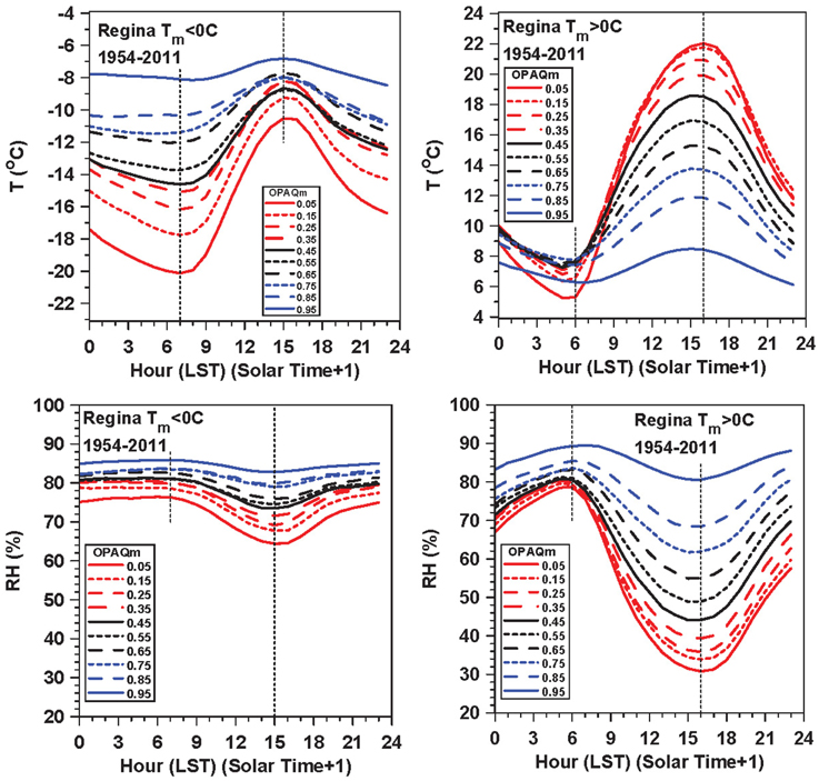
Figure 1. Diurnal cycle of T and RH as a function of opaque cloud, when T_m < 0°C (left) and (right) T_m > 0°C.

In contrast, in the warm season with T_m > 0°C, there is no snow, plants grow and transpire, increasing atmospheric water vapor. This regime is dominated by SWCF (see Figure 3 later). Minimum temperature varies little, but T_x increases and RH_m falls under clear skies (Betts et al., 2013), as the daytime solar heating drives the development of a deep unstable convective BL. We will find that in this regime LW_n depends on RH_m as well as cloud.

This difference between warm and cold seasons is a fundamental characteristic of the Prairie climate.

In Section Analysis of the BSRN Data, we will partition the BSRN data into these cold and warm seasons, and show the warm season coupling of the diurnal ranges of T and RH to ECA and LW_n. We will calibrate opaque cloud cover Regina with the LW and SW data at the nearby BSRN site. In Section Dependence of Daily Climate in Summer on Opaque Cloud and other Variables, we will expand the analysis to the full Prairie data set, focusing on summer as representative of the warm season. The cold season needs a more careful treatment, because on a daily timescale, advective temperature changes are typically larger than the solar forcing of the diurnal cycle (Betts et al., 2014b; Wang and Zeng, 2014). We will address the full diurnal cycle over the annual cycle in a later paper.

Analysis of the BSRN Data

As discussed in Section BSRN Data, we have 17 years of SW_dn and LW_dn at Bratt's Lake, Saskatchewan, which we first averaged from 1-min data to hourly means, and then to daily means, which we use here. Our analysis involves several important steps. In Sections Comparison of ERA-Interim Clear-Sky Fluxes and BSRN on Clear Days and Mean Annual Cycle of Cloud Forcing, we will compare the climatology of the daily BSRN data on nearly cloud-free days with the clear sky fluxes for the same dates from ERA-Interim (ERI), which are calculated using atmospheric temperature and humidity and climatological aerosols. Then we will represent SWC_dn by a functional fit for the annual cycle, and this will be used to compute ECA and SWCF from the BSRN data. We will compute LWCF using the ERI clear sky fluxes and the BSRN data. In Section Coupling between ECA, LW_n, DTR, and ΔRH on Daily Timescales for April to October we will show the coupling between ECA, LW_n, DTR, and ΔRH on daily timescales for the warm season. Finally we will calibrate the opaque cloud data at Regina against the near-by BSRN data for the warm and cold seasons, so we can later convert the opaque cloud data across the Prairies to both ECA and LW_n on daily timescales.

Comparison of ERA-interim Clear-sky Fluxes and BSRN on Clear Days

The ERI archive contains surface SW_dn, SW_n and the surface net clear sky flux SWC_n, but not SWC_dn so we retrieved SWC_dn by first calculating α_s from Equation (3). However, in winter with surface snow, this method fails if ERI (1-α_s) becomes very small. The surface SWC_dn has a large dependence (range 60–370 W/m²) on solar zenith angle and a small dependence (±5 W/m²) on the variable atmospheric absorption by gasses and aerosols, which are included in the ERI clear-sky computation, but are not available across the Prairies for our long-term datasets. So we looked for simplified fits to the annual profile, which neglect the variable atmospheric absorption by adjusting the empirical functions used in Betts et al. (2013). Defining DOY for Day of Year, we first fitted the ERI clear-sky shortwave data with the empirical function:

$\begin{array}{cc}{\text{SWC}}_{\text{dn}}(\text{ERIfit})=55+300\text{SIN}{(\pi \text{DS}/365)}^{1.92}& \left(12\right)\end{array}$

where DS = DOY + 14 for DOY < 351, and DOY - 351 for DOY >350 (adjusted for leap years). This fit has a mean annual bias of −0.2 ± 5.2 W/m², with mean monthly biases that are ≤ ±3 W/m².

Figure 2 (left panel) compares BSRN SW_dn for nearly clear days with ECT > 0.95 (red dots), and the ERI clear-sky SWC_dn flux (blue dots) for the same days. For these nearly clear days, the BSRN measurements are systematically higher than ERI clear sky fluxes by 9.5 ± 4.8 W/m², despite small amounts of cloud, suggesting that the reanalysis has greater absorption, either from the radiation calculation, or from less absorption by aerosols than the climatological aerosols assumed in ERI. So we shifted Equation (12) upward to define an approximate upper bound to the BSRN data:

$\begin{array}{cc}{\text{SWC}}_{\text{dn}}(\text{BSRNfit})=65+310{(\text{SIN}(\pi \text{DS}/365))}^{1.92}& \left(13\right)\end{array}$

FIGURE 2

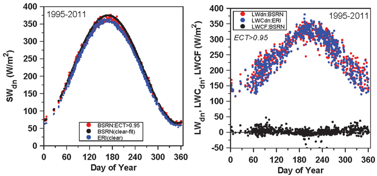
Figure 2. Clear sky (ECT>0.95) BSRN SW_dn, ERA-Interim SWC_dn and clear-sky fit used with BSRN data (left) and (right) BSRN LW_dn, ERA-Interim LWC_dn and the difference, the LWCF.

This fit, indicated by the black dots in Figure 2, is used with the BSRN SW_dn flux to calculate ECT, ECA and SWCF. The uncertainty in this fit is of the order of ±5 W/m², because it neglects the variability of atmospheric clear-sky absorption, and by aerosols. This is, however, smaller than the estimated bias of the ERI clear-sky fluxes. The data gaps in winter in Figure 2 result from the failure of our method of calculating SWC_dn on days when SW_dn is small with ERI α_s ≈ 1. As a result, the relative uncertainty in SWC_dn is larger in winter with snow than in the warm season.

For the same subset of the data, representing nearly clear skies in the daytime (ECT > 0.95), the right panel shows the measured LW_dn, the ERI clear sky flux, LWC_dn, and the LWCF from Equation (10). The annual mean LWCF for these nearly clear-sky conditions is 2.8 ± 10.5 W/m²: much smaller than the ±25 W/m² variability of LWC_dn on monthly timescales, so we will use ERI as an estimate of the clear-sky flux, LWC_dn.

Mean Annual Cycle of Cloud Forcing

Figure 3 shows the mean annual cycle of SWCF, LWCF, CF, and CF_n, binned in 0.1 ranges of ECA. There is a single bin for all the data for which ECA > 0.7, and the standard error of the bin means is shown. The top left panel just shows the variation of SWCF with ECA, which follows directly from the definitions (7) and (8). This shows that that the reduction of the surface SW flux by clouds is naturally largest in summer, when SWC_dn is largest. The sharp drop in reflective cloud cover between June and July (Betts et al., 2014a) gives the jump in the monthly mean for all data (heavy black curve).

FIGURE 3

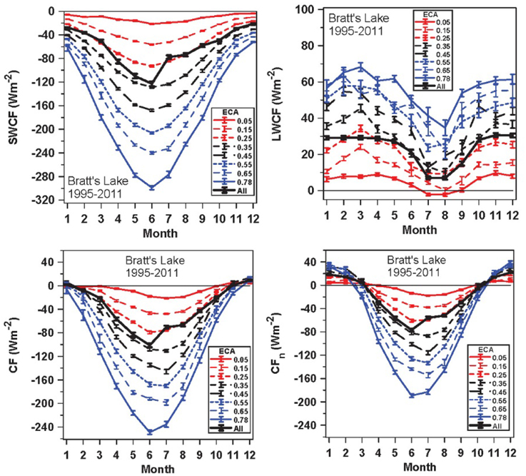
Figure 3. Mean annual cycle of SWCF, LWCF, CF, and CF_n, stratified by ECA.

The top right panel shows that the LWCF increases with ECA. The impact of clouds on the LWCF is larger in winter than in summer, when the moister atmosphere is itself more opaque to LW radiation. The very small negative values in summer for ECA = 0.05 may reflect a small positive bias in LWC_dn from ERA-Interim.

The bottom left panel is the sum of the upper two, which shows that the total cloud forcing of the down-welling flux is near zero from November to January, when SWC_dn is smallest. The bottom right panel is CF_n, the cloud forcing of the net surface radiative flux, defined by (11b). For consistency with our 1995–2011 analysis period, we used monthly mean values of surface albedo from ERA-Interim, although the annual range from 0.19 in summer to 0.61 in winter is slightly less than the range of 0.16–0.73, shown in Betts et al. (2014b) for Saskatchewan for the 2000–2001 winter. The impact of reflective snow cover in reducing the net SW fluxes means that CF_n becomes positive from November to February (Betts et al., 2013). This reversal of the sign of CF_n leads to the two distinct climate states on the Canadian Prairies for the warm and cold seasons (see Figure 1 and Betts et al., 2014b).

Coupling between ECA, LW_n, DTR, and ΔRH on daily Timescales for April to October

Following Betts et al. (2013), we will merge the warm season months, April to October with T_m > 0 and no snow cover, and show the climatology of the coupling between the SW and LW radiation field and the diurnal cycle of temperature and humidity. The Bratt's Lake site has temperature data for the full 17-year period, but RH data only for the last 12 years, 2000–2011. For this data set, we extracted T_n, T_x, RH_x, and RH_n. From SW_dn and LW_dn, we calculated ECA using Equations (7) and (13), and LW_n using (5).

The diurnal climatology is coupled to both daytime and nighttime processes. The daytime rise of temperature from T_n to T_x, and the corresponding fall of humidity from RH_x to RH_n, is driven by SW heating, as well as the surface energy partition and the growth of the unstable BL. The night-time return back to T_n and RH_x is driven by LW cooling and the structure of the stable BL (Betts, 2006). So in the daily climatology, DTR is coupled to both SW and LW processes, which are themselves coupled through the cloud field, as well as details of the BL depth and structure. The data shows the observed diurnal climatology of the coupled land-BL-cloud system. In contrast, models construct their own differing diurnal climatologies from a suite of process models and parameterizations for the surface, BL and cloud components, so this observed diurnal coupling is of value for model evaluation.

Figure 4 shows a fundamental set of relationships for the coupling between ECA, LW_n, DTR and ΔRH on daily timescales. The data has been averaged (with standard error bars) in bins of the x-axis. The upper left pair of panels shows the mean dependence of LW_n and DTR on ECA, as well as the subdivision into three RH_m ranges with roughly the same number of days: RH_m <60, 60–75, >75%.

FIGURE 4

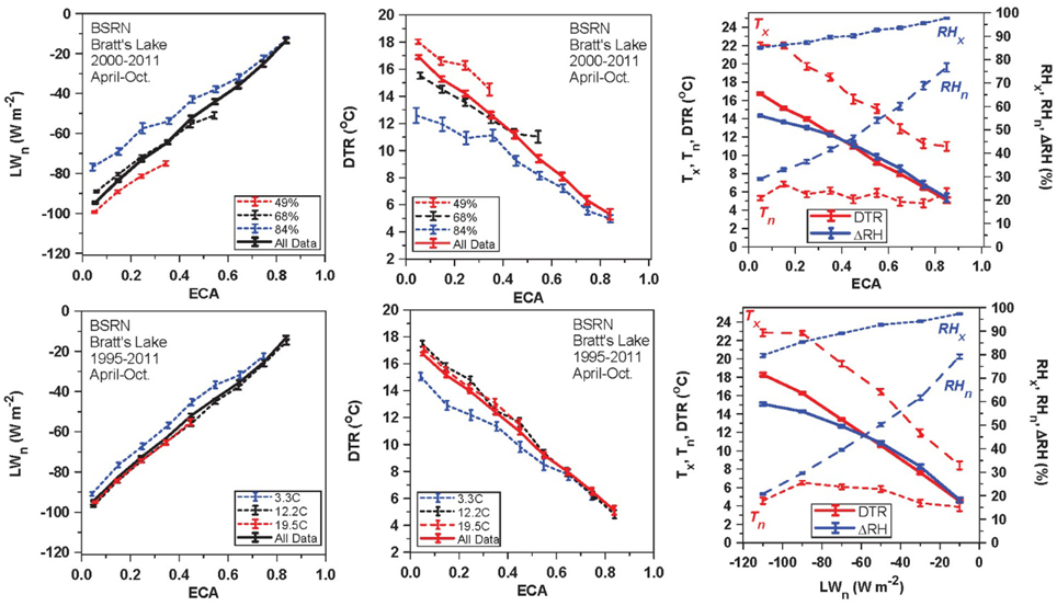
Figure 4. Coupling between ECA, LW_n, DTR, and ΔRH on daily timescales for April to October, for the BSRN station at Bratt's Lake, Saskatchewan.

The lower left pair of panels are the corresponding plots with the subdivision into three T_m ranges: 0–8, 8–16, and 16–24°C. The plots, averaging all the data, show a quasi-linear dependence of LW_n and DTR on ECA. The RH partition shows that a more humid atmosphere reduces both DTR and outgoing LW_n, consistent with reanalysis data (Betts et al., 2006). The temperature partition shows a fall of LW_n and DTR at cold mean temperatures, characteristic of April and October, with much less variability at warmer temperatures.

Multiple linear regression of daily LW_n on ECA, RH_m, and T_m gives (R² = 0.88).

$\begin{array}{cc}\begin{array}{l}{\text{LW}}_{\text{n}}=-127.7(\pm 9.3)+75.0(\pm 1.1)\text{ECA}+0.60(\pm 0.02){\text{RH}}_{\text{m}}\\ -0.26(\pm 0.03){\text{T}}_{\text{m}}\end{array}& \left(14\right)\end{array}$

The right panels show the mean dependence of DTR and ΔRH, with the corresponding maximum and minimum values, on ECA (top-right) and LW_n (bottom-right). They appear very similar, because LW_n and ECA are themselves linearly related (left panels). There is a wide seasonal range of T_x and T_n for the 7 months, but the seasonal ranges of DTR, RH_x, RH_n, and ΔRH are small (Betts et al., 2013). The standard error of the bin means for DTR and ΔRH plotted against LW_n are slightly smaller than plotted against ECA. There are 3400 days with temperature data and 2400 days with RH data, so there are generally more than a 100 days in each “All Data” bin. Values are omitted from the graphs if there are <40 days in a temperature or RH subdivision.

We conclude that the DTR increases quasi-linearly with the SW transmission represented by ECT = 1 − ECA, and with increasing outgoing LW_n, while ΔRH has a similar non-linear increase. The simple linear regression of DTR on ECA and LW_n gives:

$\begin{array}{cc}\text{DTR}=17.7(\pm 3.6)-14.8(\pm 0.3)\text{ECA}({\text{R}}^2=0.48)& \left(15\text{a}\right)\end{array}$

$\begin{array}{cc}\text{DTR}=3.2(\pm 3.1)-0.146(\pm 0.003){\text{LW}}_{\text{n}}({\text{R}}^2=0.60)& \left(15\text{b}\right)\end{array}$

We will revisit these DTR regressions later in Section Dependence of Summer Climate on ECA and LW_n with the much larger dataset for the Prairies.

The multiple regression fit including the RH_m dependence (Figure 4, top center panel), increases the explained variance substantially:

$\begin{array}{cc}\begin{array}{l}\text{DTR}=16.1(\pm 3.2)-9.0(\pm 0.4)\text{ECA}\\ -0.144(\pm 0.06)\delta {\text{RH}}_{\text{m}}({\text{R}}^2=0.60)\end{array}& \left(15\text{c}\right)\end{array}$

where δRH_m is the RH anomaly from the mean of 64.6%.

Calibrating Opaque Cloud Data at Regina to SWCF, ECA, and LW_n

The Canadian Prairie data is invaluable because of the manual observations of opaque or reflective cloud cover by trained observers over many decades. Here we map the opaque cloud impact on the surface LW and SW radiation using the BSRN data. Since these observations are hourly (with very little missing data), the daily mean, OPAQ_m, is well sampled. Betts et al. (2013) showed a one-to-one correlation between the independent daily mean opaque cloud observations at Regina and Moose Jaw, 64 km apart, which suggests that they are spatially representative for this scale. They also used measured SW_dn and LW_dn to calibrate OPAQ_m in terms of ECA and LW_n. Here we extend their analysis using the well-calibrated BSRN SW_dn and LW_dn observations. We will calibrate daily mean OPAQ_m against daily mean LW_n, as in Betts et al. (2013). However, the daily mean SWCF and ECA from (8) and (7) depend only on daytime SW reflection and absorption, so we defined a daily SW weighted OPAQSW as a weighted sum of hourly OPAQ values during daylight hours.

$\begin{array}{cc}\text{OPAQSW}=\text{SUM}(\text{SWCwt}\ast \text{OPAQ})& \left(16\right)\end{array}$

Using a simple weighting function SWCwt = A * COS(π HNoon/W)⁴ fitted to the ERI clear-sky flux data (not shown). HNoon is hours from local solar noon, and A, W are the amplitude and width (in hours) for the weighting function, which are calculated only for HNoon < ±H. We divided the year into three groups of 4 months to approximate the change of solar-day length with solar zenith angle over the annual cycle. For these groupings, NDJF, AMSO, and MJJA, the parameters (A, W, ±H) are (0.1777, 15, ±7), (0.1333, 20, ±9) and (0.1111, 24, ±11). Each weighting function sums to unity with hourly data. Across the Prairies, the difference between LST, the time-base of the climate observations, and nominal solar time ranges from 0.3 to 1.2 h for different stations in different provinces. We kept the analysis simple by choosing solar time = LST-1 for all stations.

The climate station at Regina airport is about 25 km north of the BSRN station at Bratt's Lake, so we merged the daily mean datasets for the period 1995–2011. We found significant differences between warm and cold seasons, which were well separated by sub-setting the data by daily mean temperature T_m < > 0°C, as in Figure 1.

Figure 5 (left) shows the relation between ECA derived from the BSRN data and OPAQSW, for the warm season above freezing and the cold season below freezing. ECA increases more steeply with increasing opaque cloud in the warm season than the cold season. This division is very similar if we split by the months AMJJASO and NDJFM (not shown). We show the mean and standard error of the binned data, and the quadratic regression fits to the daily data. For the warm season, these are (R² = 0.87).

FIGURE 5

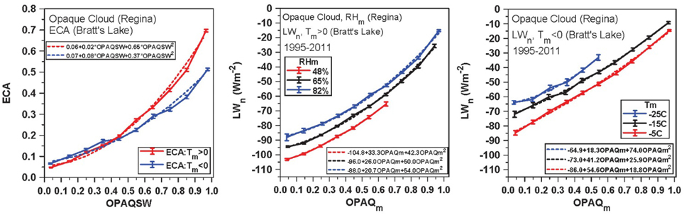
Figure 5. Relation between Opaque cloud at Regina and Bratt's Lake ECA (left), LW_n and stratified by RH_m in warm season (middle) and (right) LW_n stratified by T_m in cold season.

$\begin{array}{cc}\begin{array}{l}\text{ECA}=0.06(\pm 0.08)+0.02(\pm 0.02)\text{OPAQSW}\\ +0.65(\pm 0.02){\text{OPAQSW}}^2\end{array}& \left(17\text{a}\right)\end{array}$

For the cold season, these are (R² = 0.71).

$\begin{array}{cc}\begin{array}{l}\text{ECA}=0.07(\pm 0.11)+0.08(\pm 0.03)\text{OPAQSW}\\ +0.37(\pm 0.03){\text{OPAQSW}}^2\end{array}& \left(17\text{b}\right)\end{array}$

The uncertainty in ECA on a daily basis is of the order of ±0.08 in the warm season and ±0.11 in the cold season. The standard errors shown for the climatological fits are much smaller because they are reduced by the large number of days.

Figure 5 (middle) shows the dependence of LW_n on opaque cloud and RH_m (taken from Regina because RH was not measured at Bratt's Lake for the first 5 years) for days above freezing (3245 days). Increasing atmospheric humidity reduces the outgoing LW_n flux for the same cloud cover. The temperature dependence is very small when T_m > 0°C (not shown). In contrast for temperatures below freezing (2198 days), the humidity dependence is small but the temperature dependence is large, shown in the right panel. The outgoing LW_n flux now decreases with colder temperatures, probably because the surface cools under a stable BL in the cold season (Betts et al., 2014b).

The quadratic fits in the two right panels are the fits to the binned data. Multiple regression on the daily values of LW_n on quadratic opaque cloud and RH_m in the warm season gives (R² = 0.91).

$\begin{array}{cc}\begin{array}{l}{\text{LW}}_{\text{n}}=-128.6(\pm 7.8)+28.1(\pm 1.8){\text{OPAQ}}_{\text{m}}\\ +44.6(\pm 1.8){\text{OPAQ}}_{\text{m}}^2+0.49(\pm 0.01){\text{RH}}_{\text{m}}\end{array}& \left(18\text{a}\right)\end{array}$

Multiple regression on quadratic opaque cloud and T_m and RH_m in the cold season gives (R² = 0.83), where the contribution from RH_m is small.

$\begin{array}{cc}\begin{array}{l}{\text{LW}}_{\text{n}}=-89.2(\pm 10.1)+43.5(\pm 2.8){\text{OPAQ}}_{\text{m}}+26.8(\pm 2.5)\\ {\text{OPAQ}}_{\text{m}}^2+0.29(\pm 0.02){\text{RH}}_{\text{m}}-1.02(\pm 0.03){\text{T}}_{\text{m}}\end{array}& \left(18\text{b}\right)\end{array}$

If we merge the data for the whole year, the regression fit is (R² = 0.89).

$\begin{array}{cc}\begin{array}{l}{\text{LW}}_{\text{n}}=-112.6\pm (9.2)+34.1(\pm 1.6){\text{OPAQ}}_{\text{m}}+35.2(\pm 1.5)\\ {\text{OPAQ}}_{\text{m}}^2+0.36(\pm 0.01){\text{RH}}_{\text{m}}-0.66(\pm 0.01){\text{T}}_{\text{m}}\end{array}& \left(18\text{c}\right)\end{array}$

The incoming LW flux depends on water vapor at higher levels in the atmosphere. The addition of total column water vapor (TCWV in mm) from ERI, which is only available from 1979 on, to the multiple regression explains a little more variance, particularly in the cold season. For T<0 (R² = 0.86)

$\begin{array}{cc}\begin{array}{l}{\text{LW}}_{\text{n}}=-117.6(\pm 9.0)+39.4(\pm 2.6){\text{OPAQ}}_{\text{m}}+30.1(\pm 2.3)\\ {\text{OPAQ}}_{\text{m}}^2+0.23(\pm 0.02){\text{RH}}_{\text{m}}-1.24(\pm 0.03){\text{T}}_{\text{m}}\\ +1.38(\pm 0.07)\text{TCWV}\end{array}& \left(18\text{d}\right)\end{array}$

For the whole year the regression is (R² = 0.91).

$\begin{array}{cc}\begin{array}{l}{\text{LW}}_{\text{n}}=-118.2(\pm 8.3)+31.2(\pm 1.5){\text{OPAQ}}_{\text{m}}+37.7(\pm 1.4)\\ {\text{OPAQ}}_{\text{m}}^2+0.32(\pm 0.0){\text{RH}}_{\text{m}}-1.01(\pm 0.01){\text{T}}_{\text{m}}\\ +0.86(\pm 0.02)\text{TCWV}\end{array}& \left(18\text{e}\right)\end{array}$

Figure 6 shows the LW_n regression fits from Equation (18a) for the warm season and (18d) for the cold season. The left panel shows the dependence of LW_n on OPAQ_m, separated into three ranges of RH_m, with the regression fits from (18a) for the bin-means of RH_m. The right two panels plot the regression fits to LW_n against the BSRN LW_n from Equations (18a) and (18d). They show that OPAQ_m, a daily mean calculated from the hourly observations of opaque cloud fraction by trained observers, together with daily mean temperature, humidity and TCWV in winter, gives daily mean LW_n to about ±8–9 W/m².

FIGURE 6

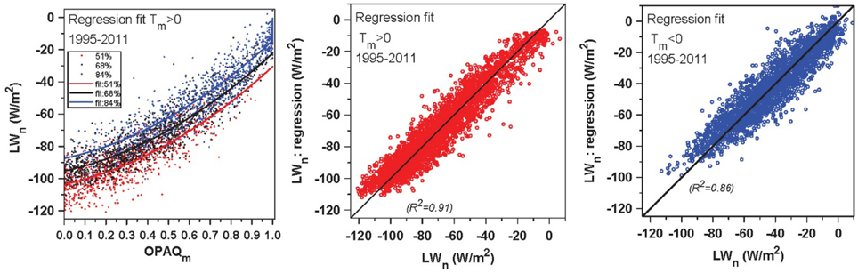
Figure 6. Regression fits based on Equation (18a) for warm season and Equation (18d) for cold season.

Figure 7 shows the raw daily data for the warm and cold season mapping between OPAQSW and BSRN ECA with the climatological regression fits from Equation (17). The uncertainty in effective cloud albedo ECA of the order of ±0.08 in the warm season means that on a daily basis, SW_n can be estimated to about ±8% from OPAQSW and SWC_dn. The uncertainty in ECA is larger in the cold season. One reason may be the larger uncertainty in SWC_dn (Section Comparison of ERA-Interim Clear-Sky Fluxes and BSRN on Clear Days), another may be that our hourly solar-weighted sampling of the cloud field, OPAQSW, involves fewer hours in the cold season than the warm season, and a third may be that with more stratiform clouds of varying thickness, rather than say warm season shallow cumulus, it is harder for observers to estimate opaque cloud fraction.

FIGURE 7

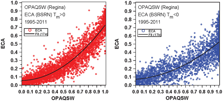
Figure 7. BSRN ECA plotted against OPAQSW at Regina for warm and cold seasons with regression fits.

Combining Equations (5) and (9) gives net radiation:

$\begin{array}{cc}{\text{R}}_{\text{n}}{=\text{ SW}}_{\text{n}}+{\text{LW}}_{\text{n}}=(1-{\alpha }_{\text{s}})(1-\text{ECA}){\text{SWC}}_{\text{dn}}+{\text{LW}}_{\text{n}}& \left(19\right)\end{array}$

Given opaque cloud cover, T_m and RH_m at climate stations, we can use the fits (17) for ECA and (18) for LW_n to estimate the climatological dependence of SW_n, LW_n, and R_n. For the summer months (JJA), SWC_dn = 343 W/m², α_s = 0.16, so an error of ±0.08 in ECA converts to an error of ±23 W/m² in SW_n. However, if the source of error is the uncertainty in the opaque cloud, which has an opposite impact on the LWCF and SWCF, the errors partly cancel in R_n. An uncertainty of ±0.1 in opaque cloud fraction at low cloud cover leads a small uncertainty in R_n of ±1 W/m², but this increases non-linearly to ±25 W/m² under nearly overcast conditions.

Dependence of Daily Climate in Summer on Opaque Cloud and Other Variables

As noted in Figure 1, warm and cold seasons differ radically in the land-atmosphere coupling. The diurnal cycle in the winter season needs careful treatment (see Section 8 of Betts et al., 2014b), which will be addressed in our next paper. Here, we just show summer (JJA) as representative of the warm season. Figure 4 shows that ECA and LW_n have a tight relationship in the warm season to the diurnal ranges of temperature and RH, which was also noted in Betts et al. (2013). We have only 17 years of the BSRN data, but we have nearly 600 station-years of the Prairie data with opaque cloud observations, which we have calibrated to ECA and LW_n with Equations (17a) and (18a). There is sufficient data in the summer season (nearly 54,000 days) to identify several local physical processes that give a systematic daily climate signal in the fully coupled surface-BL-atmosphere system. Note that the data includes all the synoptic variability that is coupled to the diurnal cycle, but our sub-setting of this large dataset extracts the daily climate signal related to specific variables. We use OPAQ_m as the primary stratification, available at all the Prairie climate stations, because of its tight coupling to LW_n and the diurnal cycle of temperature (Betts, 2006). Then we sub-stratify by relative humidity, surface wind, day-night asymmetry of the opaque cloud field and monthly precipitation anomalies. The transformation from the opaque cloud stratification to ECA and LW_n follows in Section Dependence of Summer Climate on ECA and LW_n.

Dependence of Daily Summer Climate on Opaque Cloud, Partitioned by Mean RH

Figure 8 shows the partition of the summer data for all 11 Prairie stations, most of which have record lengths over 50 years, using OPAQ_m and 5 ranges of mean RH_m (<50%, 50–60%, 60–70%, 70–80%, >80%). Figure 8 (left) shows the mean structure (with SE uncertainty) for T_x, DTR, and T_n, the middle panel shows RH_tx, RH_tn and precipitation, and the right panel shows Q_tx and θ_Etx. The magenta lines (small SE bars omitted for clarity) show the mean of the daily data without the partition into bins of RH_m. For the mean data we see that T_x, DTR, and θ_E fall with increasing cloud cover, while T_n is almost flat, while RH_tx, RH_tn, and Q_tx increase, and precipitation increases most steeply at high opaque cloud cover.

FIGURE 8

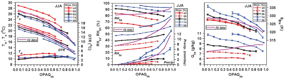
Figure 8. Dependence of T_x, DTR and T_n (left), (middle) RH_tx, RH_tn, and precipitation, (right) Q_tx and θ_Etx on opaque cloud, partitioned by RH_m.

The sub-partition into RH_m bins presents a different picture. With a drier RH_m, T_x and DTR increase systematically, but T_n only increases for very dry conditions when RH_m <50%. Perhaps this is an indicator of drought. Precipitation not surprisingly decreases with lower RH_m, becoming near zero for RH_m <50%. While RH_tx, RH_tn, and Q_tx necessarily increase with RH_m, note that Q_tx now decreases with increasing opaque cloud cover in the higher RH_m bins, despite the increase of RH_tx because of the steep fall of T_x with increasing cloud cover, and precipitation. Although θ_Etx falls with increasing cloud cover, there is an upward shift to higher θ_Etx with increasing RH_m. Conversely, while T_x increases under dry conditions, we see this gives a fall of θ_Etx for the same cloud forcing.

For the daily mean data (magenta lines), the decrease of T_x and DTR and increase of RH_tx are clearly non-linear and are well fitted with a quadratic dependence on opaque cloud (not shown). Binned by RH_m many relations become less non-linear. Figure 8 depicts the summer daily climate coupling to OPAQ_m, which together with RH_m, is coupled to LW_n. We will revisit this coupling to LW_n in Section Dependence of Summer Climate on ECA and LW_n. The variability of RH_m in summer comes from both local processes, such as changes in surface evaporation related to soil moisture or vegetation phenology, as well as remote processes, such as synoptic advection.

Dependence of Daily Summer Climate on Cloud, Partitioned by Mean Windspeed

Figure 9 shows the dependence of daily summer climate on opaque cloud, sub-stratified into four windspeed ranges (<2, 2–4, 4–6, and >6 m/s). We see that the stratification by surface windspeed shows a climate signal in both the daytime and night-time near-surface layer. At low windspeed, afternoon T_x and RH_tx are slightly higher, corresponding to a substantial increase of Q_x and θ_Etx. At sunrise under low cloud cover, T_n falls and RH_tn increases substantially with decreasing windspeed. These changes at T_n are a major contribution to the fall of the diurnal ranges of DTR and ΔRH with increasing windspeed.

FIGURE 9

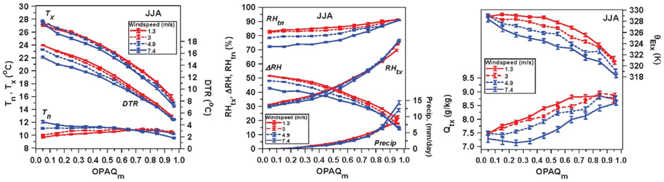
Figure 9. Coupling of daily climate to opaque cloud and windspeed.

The cooling of T_n with decreasing windspeed at low OPAQ_m is consistent with greater night-time cooling by outgoing LW_n and reduced wind-stirring, increasing the stable stratification of the night-time BL (Betts, 2006). Note there is a weak reversal at high cloud cover, when LW_n is small and the fall of surface T may be dominated by the evaporation of precipitation. The fall of RH_tn with increasing windspeed may be related to the mixing down of drier air.

At higher windspeeds in the afternoon, θ_Etx decreases with increasing cloud cover, presumably related to the reduction of the surface R_n with OPAQ_m, as well as the likelihood of low θ_E downdrafts at higher precipitation rates. However, the small increases in T_x and RH_tx with decreasing windspeed lead to a broad maximum in θ_Etx for opaque cloud <0.5 (typical of a shallow cumulus field). We can only speculate on the possible causes for this substantial increase of θ_Etx at low wind speeds. One possible reason is that the near-surface gradients in the superadiabatic layer are stronger in weak winds, giving an increase in T_x and RH_tx with respect to the mixed layer. In contrast under strong winds, there may be a near-neutral surface layer for the same cloud cover and radiative forcing. Another possible reason could be that low windspeeds may be associated with high pressure systems and with reduced advection, and the BL may drift toward a warmer and moister state on sequential days. It is also unclear whether this low windspeed increase of near-surface θ_Etx is important for convective development, but it is clearly important for convective parameterization schemes that lift near surface air to saturation to define an ascending moist adiabatic.

Dependence of Daily Summer Climate on OPAQ_m and OPAQSW

The stratifications in the previous sections were mapped in terms of OPAQ_m which is closely related to LW_n [see Equation (18a) and Section Dependence of Summer Climate on ECA and LW_n]. This section will show how the diurnal cycle changes if the opaque cloud fraction is non-uniform between day and night, so it has a different impact on SW_n and LW_n which in turn changes R_n given by (19). We define:

$\begin{array}{cc}\Delta \text{OPAQ}={\text{OPAQ}}_{\text{m}}-\text{OPAQSW}& \left(20\right)\end{array}$

When ΔOPAQ > 0, it is less cloudy in the daytime hours than at night, which gives a positive change to both SWCF and LWCF, as well as R_n, with the reverse for ΔOPAQ < 0. It is generally cloudier in the daytime in summer with a mean value of ΔOPAQ = −0.04.

Figure 10 shows the diurnal cycle impact for three ranges: ΔOPAQ <−0.5, −0.5< ΔOPAQ <0.5 and ΔOPAQ >0.5. The mean values of ΔOPAQ for these three bins are −0.13, 0.00, +0.11. As expected, as ΔOPAQ increases, both T_x and T_n increase (left panel), but the response of DTR is an increase when OPAQ_m is high, but the change is not well-defined when OPAQ_m is low. For ΔOPAQ < 0, RH increases, and the decrease of ΔRH with OPAQ_m becomes steeper. The right panel shows that daily R_n and afternoon θ_E both increase with increasing ΔOPAQ: suggesting that the increase of afternoon θ_E can be viewed as a coupled response to less daytime cloud and higher daily R_n. The small associated increase of precipitation, shown in the middle panel is consistent with this increase of afternoon θ_E.

FIGURE 10

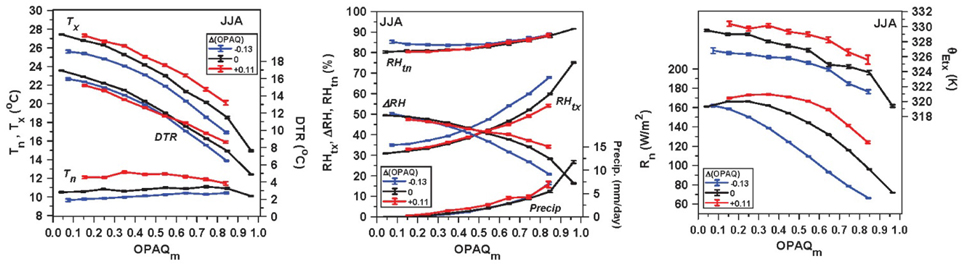
Figure 10. Coupling of daily climate to OPAQ_m and ΔOPAQ.

Dependence of Daily Summer Climate on Cloud, Partitioned by Precipitation Anomalies

The land-atmosphere coupling depends on two key processes: R_n which mostly depends on cloud forcing, and the partition of R_n into sensible and latent heat fluxes which depends on the availability of soil water, as well as vegetation phenology and rooting. In this climate dataset we have no measurements of soil water (or phenology), but we explored whether precipitation anomalies could provide some information on the availability of soil water, and hence the energy partition and the daily climate. Betts et al. (2014a) showed that summer afternoon RH_tx and P_LCLtx anomalies are strongly correlated on monthly timescales with precipitation anomalies for the current month and preceding 2 months (Mo-1 and Mo-2), as well as the current month opaque cloud anomalies. For MJJA they found using multiple linear regression (with R² = 0.68).

$\begin{array}{cc}\begin{array}{l}\delta {\text{RH}}_{\text{tx}}=4.21(\pm 0.12)\delta \text{PrecipWT}\\ +4.46(\pm 0.10)\delta \text{OpaqueCloud}\end{array}& \left(21\right)\end{array}$

with δOpaqueCloud in tenths, and δPrecipWT in mm/day, given by:

$\begin{array}{cc}\begin{array}{l}\delta \text{PrecipWT}=0.17(\pm 0.02)\ast \delta \text{Precip}(\text{Mo}-2)+0.35(\pm 0.02)\ast \\ \delta \text{Precip}(\text{Mo}-1)+0.48(\pm 0.02)\ast \delta \text{Precip}\end{array}& \left(22\right)\end{array}$

Within the uncertainty of ±0.02, these weighting coefficients are the same for the P_LCLtx regression; both for MJJA and for the subset of the summer months, JJA. So this weighted precipitation contains monthly timescale information about the memory of the current climate to current and past precipitation. We can suppose that this correlation with RH_tx means that these monthly values of δPrecipWT are related to soil water anomalies. The reasoning here is that we know from surface flux measurements (e.g., Betts and Ball, 1995, 1998) as well as many model studies that there is a chain of processes linking soil water to surface vegetative resistance and transpiration, to the vapor pressure deficit and the LCL of near-surface air (Betts, 2000, 2004, 2009; Betts et al., 2004; Betts and Viterbo, 2005; Seneviratne et al., 2010; van Heerwaarden et al., 2010; Ferguson et al., 2012).

For this paper, we calculated the monthly precipitation anomalies for each station from a mean monthly precipitation climatology, found by combining the 11 stations. Then we used Equation (22) to compute monthly weighted anomalies δPrecipWT for each station. These were used to sort the daily data. This is more primitive than using a vegetation model and daily soil water balance model, but it has the advantage of being entirely observationally based. But the mismatch between the monthly and daily timescales introduces a significant approximation, because we use δPrecipWT for sorting all the days in the current month, regardless of when it rains during this month. Nonetheless useful climate results will emerge from these composites because the dataset is so large.

Mean Daily Climate Dependence on δPrecipWT

Figure 11 shows how the mean daily climate and cloud cover changes with increasing δPrecipWT. The rather small standard errors shown for many variables reflect the very large number of days in this dataset. The left panel shows that T_x and DTR fall by 3.4 and 2.8°C respectively with increasing δPrecipWT, while T_n changes very little (Betts et al., 2013). The center panel shows that as δPrecipWT increases, opaque cloud cover increases by 10%, while afternoon RH_tx and sunrise RH_tn increase by 16 and 11%, so that the diurnal range ΔRH decreases. The right panel shows the large fall of P_LCLtx (71 hPa), and very little systematic change of mean θ_Etx. With the increasing cloud cover, SW_n decreases by 18 W/m², but there is also a decrease in outgoing LW_n (not shown), so that R_n decreases by only 2 W/m². These climate signals are consistent with increasing evaporation as δPrecipWT and presumably soil water increase.

FIGURE 11

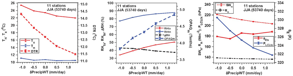
Figure 11. Dependence of mean diurnal climate, opaque cloud, and radiation on δPrecipWT.

Stratification of Daily Summer Climate by Opaque Cloud and δPrecipWT

Figure 12 shows the stratification of the daily climate by opaque cloud and δPrecipWT. The partition by δPrecipWT at constant OPAQ_m changes R_n by < ± 4 W/m², so the change of diurnal climate can be interpreted as the impact of δPrecipWT on the partition of R_n.

FIGURE 12

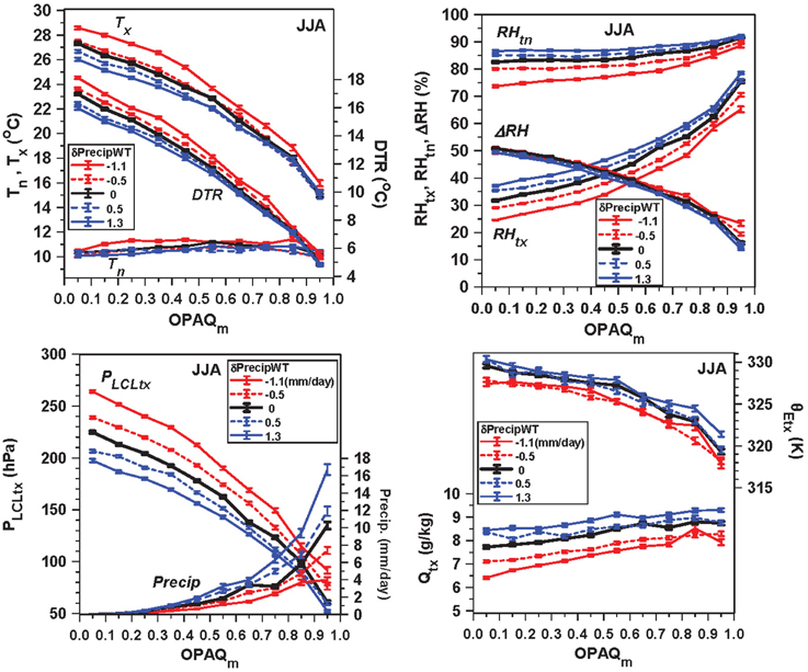
Figure 12. Stratification of daily climate by opaque cloud and δPrecipWT.

Figure 12 (top left) shows that as the monthly anomaly of δPrecipWT increases at constant cloud cover, T_x and DTR both fall on the daily timescale, with the largest changes at low cloud cover, while T_n changes little. The top right panel shows that both RH_tx and RH_tn increase with increasing δPrecipWT, but ΔRH falls slightly. The bottom left panel shows the corresponding steep fall of P_LCLtx (representative of afternoon cloud-base) and increase in daily mean precipitation, which is to be expected since precipitation for the current month is almost half the contribution to δPrecipWT in Equation (22). The bottom right panel shows that the drop of T_x, coupled with the substantial rise of RH_tx with δPrecipWT, results in an a relatively large increase of Q_tx and a smaller increase of θ_Etx.

This shift with increasing δPrecipWT toward a cooler, moister afternoon daily climate with a lower cloud-base and a slightly higher θ_Etx, is consistent with increased evaporation from soils that are moister, due to higher precipitation on the monthly to seasonal timescale. Comparing with Figure 8, where the data were simply stratified by daily RH_m, we see some similarities, but also important differences. For example, Figure 12 shows the increase of Q_tx consistent with larger precipitation anomalies and increased evaporation, which is different from the simple RH stratification in Figure 8.

Dependence of Summer Climate on ECA and LW_n

This section addresses the remapping of the results shown in Section Dependence of Daily Climate in Summer on Opaque Cloud and other Variables from opaque cloud back to daily mean ECA and LW_n using the regression relations (17a) and (18a). This is so we can compare the full Prairie dataset with the BSRN data in Figure 4. Figure 13 has six panels corresponding to the ECA (top row) and LW_n (bottom row) dependence of T_x, T_n, and DTR for the RH_m, windspeed and precipitation anomaly stratifications shown in Figures 8, 9, 12. For T_x and DTR, the left pair also shows the mean of all the data (magenta).

FIGURE 13

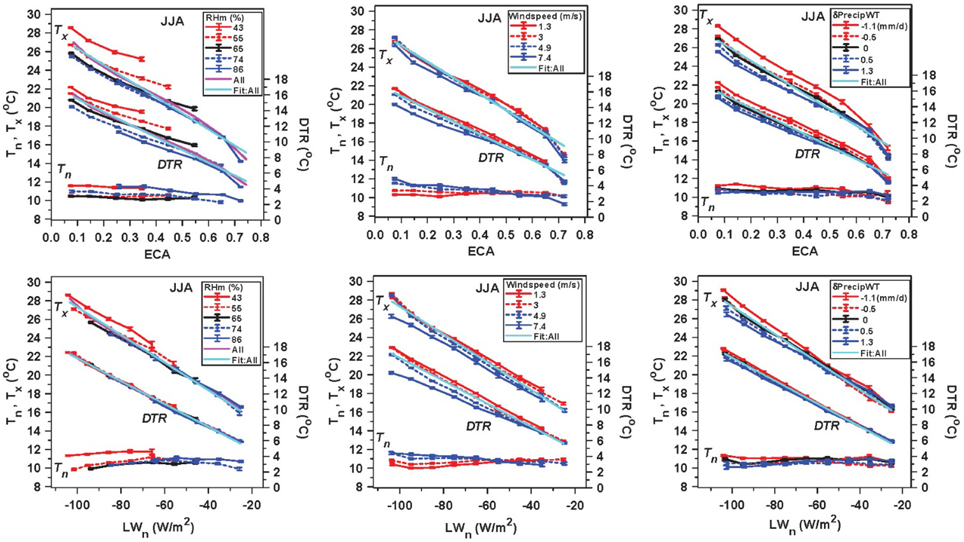
Figure 13. ECA (upper row) and LW_n (lower row) dependence of T_x, T_n, and DTR for the RH_m, windspeed and precipitation anomaly stratifications.

The top row of panels differ from the corresponding panels in Figures 8, 9, 12 by a small difference between OPAQ_m and OPAQSW and the quadratic transformation from OPAQSW to ECA given by (17a). However, the transformation (18a) from OPAQ_m to LW_n also includes a substantial RH_m dependence, which has a big impact on the stratifications that involve RH differences. The bottom left panel for the RH_m partition shows a collapse of DTR into almost a single line against LW_n and the bottom right for the precipitation partition shows a similar but smaller change. Both show a reduction in the spread of T_x, when plotted against LW_n. One interpretation of these differences between these ECA and LW_n stratifications is that the cooling at night is directly coupled to the LW_n, but the daytime partition of the solar flux determines the daytime warming and this is correlated to either RH_m or the precipitation anomalies. In contrast, the middle pair shows that the spread of DTR and T_x is slightly increased when plotted against LW_n rather than ECA, which is related to the small increase in RH with decreasing windspeed.

We have recovered for this much larger summer dataset, the nearly linear dependence of DTR on ECA and LW_n, which was seen in Figure 4 for 12 years of data at a single site for the warm season (AMJJAS). The linear regression fits to the full set of filtered daily data (53,740 days) are shown in all panels (cyan):

$\begin{array}{cc}\text{DTR}=17.10(\pm 0.02)-16.29(\pm 0.07)\ast \text{ECA}({\text{R}}^2=0.53)& \left(23\right)\end{array}$

$\begin{array}{cc}\text{DTR}=1.95(\pm 0.04)-0.146(\pm 0.001)\ast {\text{LW}}_{\text{n}}({\text{R}}^2=0.61)& \left(24\right)\end{array}$

$\begin{array}{cc}{\text{T}}_{\text{x}}=28.05(\pm 0.03)-17.35(\pm 0.09)\ast \text{ECA}({\text{R}}^2=0.41)& \left(25\right)\end{array}$

$\begin{array}{cc}{\text{T}}_{\text{x}}=12.42(\pm 0.06)-0.149(\pm 0.001)\ast {\text{LW}}_{\text{n}}({\text{R}}^2=0.44)& \left(26\right)\end{array}$

The explained variance is much higher for DTR than T_x, because DTR = T_x − T_n and this difference removes much of the daily variability related to the seasonal cycle and synoptic scale variability. Comparing Equations (15a) and (15b) with (23) and (24) we see that DTR has the same slope with LW_n, while this larger Prairie data set has a larger slope with ECA. Clearly the linear fit is better for the LW_n plots, confirming observationally the strong coupling between DTR and daily LW_n seen in models (Betts, 2004, 2006). The regression of this larger data set on ECA and the anomaly δRH_m (from the mean of 63.5%) is:

$\begin{array}{cc}\begin{array}{l}\text{DTR}=16.30(\pm 0.06)-12.60(\pm 0.08)\text{ECA}\\ -0.083(\pm 0.001)\delta {\text{RH}}_{\text{m}}({\text{R}}^2=0.57)\end{array}& \left(27\right)\end{array}$

Comparing with Equation (15c) we see here a larger slope with ECA and a reduced dependence on δRH_m.

The windspeed dependence of DTR in the center panels increases with decreasing cloud or increasing transmission ECT. We can represent this by adding a term to the multiple linear regression for the product of ECT and the anomaly δWS (from the mean of 3.45 m/s). This gives with a small increase in the explained variance to R² = 0.63.

$\begin{array}{cc}\begin{array}{l}\text{DTR}=2.02(\pm 0.04)-0.145(\pm 0.000){\text{LW}}_{\text{n}}\\ -0.43(\pm 0.01)\text{ECT}\ast \delta \text{WS}\end{array}& \left(28\right)\end{array}$

So DTR falls with increasing windspeed by −0.43 K/(ms⁻¹) under clear skies.

The δPrecipWT dependence of DTR and T_x in the bottom right panel is small, with regressions:

$\begin{array}{cc}\begin{array}{l}\text{DTR}=2.12(\pm 0.04)-0.144(\pm 0.001)\ast {\text{LW}}_{\text{n}}\\ +0.30(\pm 0.01)\delta \text{PrecipWT}({\text{R}}^2=0.61)\end{array}& \left(24\text{a}\right)\end{array}$

$\begin{array}{cc}\begin{array}{l}{\text{T}}_{\text{x}}=12.702(\pm 0.06)-0.146(\pm 0.001)\ast {\text{LW}}_{\text{n}}\\ +0.47(\pm 0.02)\delta \text{PrecipWT}({\text{R}}^2=0.44)\end{array}& \left(26\text{a}\right)\end{array}$

Figure 14 shows the nearly linear dependence of RH_tx and P_LCLtx on LW_n, partitioned by daily windspeed and weighted monthly precipitation anomaly.

FIGURE 14

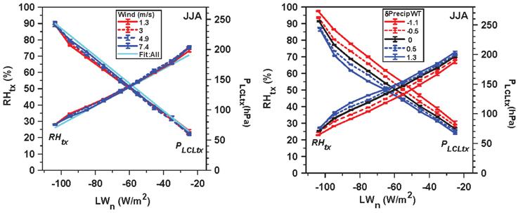
Figure 14. LW_n dependence of RH_tx and P_LCLtx, for the windspeed and precipitation anomaly stratifications.

The left panel also shows the linear regression fits (cyan) for all the daily data, which are:

$\begin{array}{cc}{\text{RH}}_{\text{tx}}=84.8(\pm 0.1)+0.566(\pm 0.002){\text{LW}}_{\text{n}}(R^2=0.67)& \left(29\right)\end{array}$

$\begin{array}{cc}{\text{P}}_{\text{LCLtx}}=7.5(\pm 0.6)-2.27(\pm 0.01){\text{LW}}_{\text{n}}({\text{R}}^2=0.65)& \left(30\right)\end{array}$

For the right panel, adding δPrecipWT (in mm/day), the multiple linear regression gives:

$\begin{array}{cc}\begin{array}{l}{\text{RH}}_{\text{tx}}=82.9(\pm 0.1)+0.550(\pm 0.002){\text{LW}}_{\text{n}}\\ +3.32(\pm 0.05)\delta \text{PrecipWT}({\text{R}}^2=0.69)\end{array}& \left(31\right)\end{array}$

$\begin{array}{cc}\begin{array}{l}{\text{P}}_{\text{LCLtx}}=16.5(\pm 0.5)-2.16(\pm 0.01){\text{LW}}_{\text{n}}\\ -15.5(\pm 0.2)\delta \text{PrecipWT}({\text{R}}^2=0.69)\end{array}& \left(32\right)\end{array}$

These linear regression fits for RH_x have a higher R² than the linear fits of DTR on LW_n. For fixed LW_n, a 1 mm/day increase in the monthly precipitation anomaly increases daily RH_tx by 3.3% and decreases P_LCLtx by 15.5 hPa.

Derived from nearly 54,000 days of observations, these linear regression fits characterize the coupled surface-BL-cloud system over the Prairies on daily timescales, where the afternoon LCL is closely related to cloud-base (Betts et al., 2013), and LW_n is tightly coupled to opaque cloud fraction (Figure 6). For model evaluation, this set of relationships, (24) and (28)–(32), describing the quasi-linear coupling between LW_n and the key diurnal climate variables DTR, RH_tx, and P_LCLtx, may be the most useful.

Summary and Conclusions

The Prairie data show the observed diurnal climatology of the coupled land-BL-cloud system. In contrast, models construct their own differing diurnal climatologies from a suite of process models and parameterizations for the surface, BL and cloud components. Our broad intent is to provide quantitative guidance based on observations for the evaluation of both simplified models, and the large-scale models that we depend upon for weather forecasting and climate simulation. The control of radiation by SWCF and LWCF is dominant on daily timescales (Betts et al., 2013), although both cloud and precipitation matter on monthly to seasonal timescales (Betts et al., 2014a). So understanding hydrometeorology requires both precipitation and cloud/radiation measurements as well as temperature, RH and pressure data. Temperature, RH and pressure are all needed, because from them we can compute Q, LCL, and θ_E, which feedback on clouds and precipitation in the warm season. This paper has focused primarily on mapping the coupling of clouds and other observables to the daily climate in the warm season.

We used the Canadian Prairie data from eleven climate stations, which contain nearly 600 station-years of well-calibrated relatively homogenous data. Earlier work (Betts et al., 2013) explored the coupling between daily climate and opaque cloud cover over the annual cycle, and used SW_dn and LW_dn measurements to calibrate the opaque cloud observations in terms of SWCF and LW_n. This paper has extended their analysis in several directions. First we noted that the warm and cold season regimes are sharply delineated by the freezing point of water. The diurnal cycle in the winter cold regime with surface snow is dominated by LWCF, so that near-surface minimum temperatures plunge under clear skies. In contrast, when T>0°C, SWCF dominates and maximum temperatures rise in clear skies, while minimum temperatures change little. With this framework, we revisited the calibration of the opaque cloud data in both cold and warm seasons using the high quality BSRN data from Bratt's Lake, Saskatchewan. Using just the BSRN data we explored the dependence of the diurnal range of T and RH on the radiative drivers. We confirmed the nearly linear dependence of DTR on both ECA and LW_n in the warm season, seen in Betts et al. (2013), and earlier in model data (Betts, 2006). We then used multiple regression to relate opaque cloud data at Regina with ECA and LW_n at Bratt's Lake, only 25 km away. We found that LW_n could be determined from the daily means of OPAQ_m and RH_m to ±8 W/m² (R² = 0.91) in the warm season (T > 0°C); and from the daily means of OPAQ_m, T_m, RH_m, and TCWV to ±9 W/m² (R² = 0.86) in the cold season (T < 0°C). We derived quadratic relationships between OPAQSW, opaque cloud weighted by the daytime clear-sky SW_dn flux, which give effective cloud albedo, ECA to ±0.08 (R² = 0.87) in the warm season, and to ±0.11 (R² = 0.71) in the cold season.

We applied these relations between OPAQ_m and LW_n, and OPAQSW and ECA to all eleven Prairie stations, and created a summer (JJA) merge of the eleven Prairie stations to explore sub-stratifications of the Prairie data. As noted by Betts et al. (2013, 2014a), cloud cover is the primary driver of daily climate, as it largely determines LW_n and R_n. However, the additional sub-stratification by RH_m, windspeed, the day-night asymmetry of cloud cover and monthly precipitation anomalies show how other physical processes are coupled to daily land-surface climate in summer.

The RH stratification shows that T_x and DTR increase systematically with drier RH_m, but T_n only increases for very low RH_m <50%. Precipitation not surprisingly decreases sharply with lower RH_m, becoming near zero for RH_m <50%. While θ_Etx falls with increasing cloud cover, as T_x falls, there is an upward shift with constant cloud but increasing RH_m to higher θ_Etx, consistent with increasing precipitation. The variability of RH_m in summercomes from both remote processes, such as synoptic advection, as well as local processes, such as changes in surface evaporation related to soil moisture or vegetation phenology.

The surface windspeed stratification has an impact on both the daytime and night-time near-surface layer. At low windspeed, afternoon T_x and RH_tx are slightly higher, giving a substantial increase of Q_x and θ_Etx. One possible reason is that the near-surface gradients in the superadiabatic layer are stronger in weak winds, giving an increase in T_x and RH_tx relative to the mixed layer. In contrast under strong winds, there may be a near-neutral surface layer for the same cloud cover and radiative forcing. It is unclear whether this low windspeed increase of near-surface θ_Etx is important for convective development. At sunrise, T_n is lower and RH_tn is higher at low windspeed and low cloud cover, consistent with greater night-time cooling by outgoing LW_n and reduced wind-stirring giving a more stable stratification in the night-time BL (Betts, 2006). The fall of the diurnal ranges of DTR and ΔRH with increasing windspeed are heavily influenced by these changes at T_n. The fall of RH_tn with increasing windspeed may be related to the mixing down of drier air into the stable BL.

The difference, ΔOPAQ, between the two opaque cloud means, daily mean OPAQ_m (closely related to LW_n) and OPAQSW, weighted by the solar clear sky flux (and related to ECA), is a measure of the asymmetry of the cloud field between day and night. ΔOPAQ > 0 means it is less cloudy in the daytime hours than at night giving more solar heating and less LW cooling at night. We used ΔOPAQ to sub-stratify the data. As expected, as ΔOPAQ increases, both T_x and T_n increase, but the response of DTR is more complex. DTR increases when OPAQ_m is high, but the change is not well-defined when OPAQ_m is low. We see that daily R_n and afternoon θ_E both increase with increasing ΔOPAQ, and there is a small associated increase of precipitation.

The land-atmosphere coupling depends on two key processes: R_n that mostly depends on cloud forcing, which we know quite well from the opaque cloud data, and the partition of R_n into sensible and latent heat fluxes, which depends on the availability of soil water, as well as vegetation phenology. In this dataset we have no measurements of soil water or phenology, but based on the work of Betts et al. (2014a) we sub-stratified the data using monthly weighted precipitation anomalies as a surrogate for soil moisture anomalies. We found a shift with increasing precipitation anomalies toward cooler, moister afternoon daily climate with a lower cloud-base and a higher θ_Etx. This is consistent with increased evaporation from soils that are moister because of higher precipitation on the monthly to seasonal timescale.

Finally we remapped the diurnal changes of temperature from the stratifications based on RH_m, wind and precipitation anomalies back onto LW_n and ECA. Because LW_n is itself dependent on RH_m in the warm season, the relationship between DTR and LW_n becomes almost independent of RH_m and precipitation anomalies. This confirms the fundamental importance of daily LW_n in determining the diurnal temperature range (Betts, 2006), independent of the evaporative and advective processes that modify RH. However, the afternoon RH_tx retains a substantial dependence on precipitation anomalies. We map the quasi-linear coupling between LW_n and the key diurnal climate variables DTR, RH_tx, and P_LCLtx using multiple linear regression in Equations (24) and (28)–(32), with R²-values ranging from 0.61 to 0.69. These relationships derived from the Prairie daily climate data for this fully coupled system may be the most useful for model evaluation. Although we also derived relationships using multiple linear regression between DTR and ECA and RH_m, further exploration of the daytime forcing of the diurnal climate requires the partition of R_n into sensible and latent heat fluxes. We plan to extend this work using surface flux products for the Canadian Prairies (Wang et al., 2013).

Conflict of Interest Statement

The Guest Associate Editor Dr. Pierre Gentine declares that, despite having collaborated with author Dr. Alan K. Betts, the review process was handled objectively. The authors declare that the research was conducted in the absence of any commercial or financial relationships that could be construed as a potential conflict of interest.

Acknowledgments

This research was supported by Agriculture and Agri-Food Canada and the Center for Ocean-Land-Atmosphere Studies, George Mason University. We thank the civilian and military technicians of the Meteorological Service of Canada and the Canadian Forces Weather Service, who have made reliable cloud observations hourly for 60 years. We thank Devon Worth for processing the Prairie climate data and Jeffrey Watchorn for processing the BSRN data. The daily mean data are available from the corresponding author. The full hourly dataset is being reprocessed and will available later this year.

References

Abramowitz, G. (2012). Towards a public, standardized, diagnostic benchmarking system for land surface models. Geosci. Model Dev. 5, 819–827. doi: 10.5194/gmd-5-819-2012

CrossRef Full Text | Google Scholar

Beljaars, A. C. M., Viterbo, P., Miller, M. J., and Betts, A. K. (1996). The anomalous rainfall over the United States during July 1993: sensitivity to land surface parameterization and soil moisture anomalies. Mon. Weather Rev. 124, 362–383.

Google Scholar

Betts, A. K. (2000). Idealized model for equilibrium boundary layer over land. J. Hydrometeorol. 1, 507–523. doi: 10.1175/1525-7541(2000)001<0507:IMFEBL>2.0.CO;2

CrossRef Full Text | Google Scholar

Betts, A. K. (2004). Understanding hydrometeorology using global models. Bull. Am. Meteorol. Soc. 85, 1673–1688. doi: 10.1175/BAMS-85-11-1673

CrossRef Full Text | Google Scholar

Betts, A. K. (2006). Radiative scaling of the nocturnal boundary layer and the diurnal temperature range. J. Geophys. Res. 111, D07105. doi: 10.1029/2005JD006560

CrossRef Full Text | Google Scholar

Betts, A. K. (2007). Coupling of water vapor convergence, clouds, precipitation, and land-surface processes. J. Geophys. Res. 112, D10108. doi: 10.1029/2006JD008191

CrossRef Full Text | Google Scholar

Betts, A. K. (2009). Land-surface-atmosphere coupling in observations and models. J. Adv. Model Earth Syst. 1, 18. doi: 10.3894/JAMES.2009.1.4

PubMed Abstract | Full Text | CrossRef Full Text | Google Scholar

Betts, A. K., and Ball, J. H. (1995). The FIFE surface diurnal cycle climate. J. Geophys. Res. 100, 25679–25693. doi: 10.1029/94JD03121

CrossRef Full Text | Google Scholar

Betts, A. K., and Ball, J. H. (1998). FIFE surface climate and site-average dataset: 1987-1989. J. Atmos Sci. 55, 1091–1108.

Google Scholar

Betts, A. K., Ball, J. H., Barr, A. H., Black, T. A., McCaughey, J. H., and Viterbo, P. (2006). Assessing land-surface-atmosphere coupling in the ERA-40 reanalysis with boreal forest data. Agric. For. Meteorol. 140, 355–382. doi: 10.1016/j.agrformet.2006.08.009

CrossRef Full Text | Google Scholar

Betts, A. K., Desjardins, R., and Worth, D. (2013). Cloud radiative forcing of the diurnal cycle climate of the Canadian Prairies. J. Geophys. Res. Atmos. 118, 8935–8953. doi: 10.1002/jgrd.50593

CrossRef Full Text | Google Scholar

Betts, A. K., Desjardins, R., Worth, D., and Beckage, B. (2014a). Climate coupling between temperature, humidity, precipitation and cloud cover over the Canadian Prairies. J. Geophys. Res. Atmos. 119, 13305–13326. doi: 10.1002/2014JD022511

CrossRef Full Text | Google Scholar

Betts, A. K., Desjardins, R., Worth, D., Wang, S., and Li, J. (2014b). Coupling of winter climate transitions to snow and clouds over the Prairies. J. Geophys. Res. Atmos. 119, 1118–1139. doi: 10.1002/2013JD021168

CrossRef Full Text | Google Scholar

Betts, A. K., Helliker, B., and Berry, J. (2004). Coupling between CO₂, water vapor, temperature and radon and their fluxes in an idealized equilibrium boundary layer over land. J. Geophys. Res. 109, D18103. doi: 10.1029/2003JD004420

CrossRef Full Text | Google Scholar

Betts, A. K, and Viterbo, P. (2005). Land-surface, boundary layer and cloud-field coupling over the south-western Amazon in ERA-40. J. Geophys. Res. 110, D14108. doi: 10.1029/2004JD005702

CrossRef Full Text | Google Scholar

Dirmeyer, P. A. (2006). The hydrologic feedback pathway for land–climate coupling. J. Hydrometeor. 7, 857–867. doi: 10.1175/JHM526.1

CrossRef Full Text | Google Scholar

Dirmeyer, P. A., Koster, R. D., and Guo, Z. (2006). Do Global models properly represent the feedback between land and atmosphere? J. Hydrometeor. 7, 1177–1198. doi: 10.1175/JHM532.1

CrossRef Full Text | Google Scholar

Dirmeyer, P. A., Wang, Z., Mbuh, M. J., and Norton, H. E. (2014). Intensified land surface control on boundary layer growth in a changing climate. Geophys. Res. Lett. 41, 1290–1294. doi: 10.1002/2013GL058826

CrossRef Full Text | Google Scholar

Eltahir, E. A. B. (1998). A soil moisture–rainfall feedback mechanism: 1. Theory and observations. Water Resour. Res. 34, 765–776. doi: 10.1029/97WR03499

CrossRef Full Text | Google Scholar

Ferguson, C. R., and Wood, E. F. (2011). Observed land–atmosphere coupling from satellite remote sensing and reanalysis. J. Hydrometeorol. 12, 1221–1254. doi: 10.1175/2011JHM1380.1

CrossRef Full Text | Google Scholar

Ferguson, C. R., Wood, E. F., and Vinukollu, R. K. (2012). A global intercomparison of modeled and observed land-atmosphere coupling. J. Hydrometeorol. 13, 749–784. doi: 10.1175/JHM-D-11-0119.1

CrossRef Full Text | Google Scholar

Findell, K. L., and Eltahir, E. A.B. (2003). Atmospheric controls on soil moisture–boundary layer interactions. Part I: framework development. J. Hydrometeor. 4, 552–569. doi: 10.1175/1525-7541(2003)004<0552:ACOSML>2.0.CO;2

CrossRef Full Text | Google Scholar

Flato, G., Marotzke, J., Abiodun, B., Braconnot, P., Chou, S. C., Collins, W., et al. (2013). “Evaluation of climate models,” in Climate Change 2013: The Physical Science Basis. Contribution of Working Group I to the Fifth Assessment Report of the Intergovernmental Panel on Climate Change, eds T. F. Stocker, D. Qin, G.-K. Plattner, M. Tignor, S. K. Allen, J. Doschung, A. Nauels, Y. Xia, V. Bex, and P. M. Midgley (Cambridge; New York, NY: Cambridge University Press), 741–882. doi: 10.1017/CBO9781107415324.020

CrossRef Full Text

Guo, Z. C., Koster, R. D., Dirmeyer, P. A., Bonan, G., Chan, E., Cox, P., et al. (2006). GLACE: the global land–atmosphere coupling experiment. Part II: analysis. J. Hydrometeor. 7, 611–625. doi: 10.1175/JHM511.1

CrossRef Full Text | Google Scholar

Koster, R. D., Dirmeyer, P. A., Guo, Z., Bonan, G., Chan, E., Cox, P., et al. (2004). Regions of strong coupling between soil moisture and precipitation. Science 305, 1138–1140. doi: 10.1126/science.1100217

PubMed Abstract | Full Text | CrossRef Full Text | Google Scholar

Koster, R. D., Guo, Z., Dirmeyer, P. A., Bonan, G., Chan, E., Cox, P., et al. (2006). GLACE: the global land–atmosphere coupling experiment. Part I: overview. J. Hydrometeor. 7, 590–610. doi: 10.1175/JHM510.1

CrossRef Full Text | Google Scholar

Koster, R. D., and Manahama, S. P. P. (2012). Land surface controls on hydroclimatic means and variability. J. Hydrometeor. 13, 1604–1619. doi: 10.1175/JHM-D-12-050.1

CrossRef Full Text | Google Scholar

Koster, R. D., and Suarez, M. J. (2001). Soil moisture memory in climate models. J. Hydrometeor. 2, 558–570. doi: 10.1175/1525-7541(2001)002<0558:SMMICM>2.0.CO;2

CrossRef Full Text | Google Scholar

MANOBS. (2013). Environment Canada MANOBS, Chapter 1, Sky. Available online at http://www.ec.gc.ca/manobs/default.asp?lang=En&n=A1B2F73E-1.

Santanello, J. A., Peters-Lidard, C. D., Kennedy, A., and Kumar, S. V. (2013). Diagnosing the nature of land–atmosphere coupling: a case study of dry/wet extremes in the U.S. Southern great plains. J. Hydrometeor. 14, 3–24. doi: 10.1175/JHM-D-12-023.1

CrossRef Full Text | Google Scholar

Seneviratne, S. I., Corti, T., Davin, E. L., Hirschi, M., Jaeger, E. B., Lehner, I., et al. (2010). Investigating soil moisture-climate interactions in a changing climate: a review. Earth Sci. Rev. 99, 125–161. doi: 10.1016/j.earscirev.2010.02.004

CrossRef Full Text | Google Scholar

Taylor, C. M., Birch, C. E., Parker, D. J., Dixon, N., Guichard, F., Nikulin, G., et al. (2013). Modeling soil moisture-precipitation feedback in the Sahel: importance of spatial scale versus convective parameterization. Geophys. Res. Lett. 40, 6213–6218. doi: 10.1002/2013GL058511

CrossRef Full Text | Google Scholar

van Heerwaarden, C. C., Vilà Guerau de Arellano, J., Gounou, A., Guichard, F., and Couvreux, F. (2010). Understanding the daily cycle of evapotranspiration: a method to quantify the influence of forcings and feedbacks. J. Hydrometeor. 11, 1405–1422. doi: 10.1175/2010JHM1272.1

CrossRef Full Text | Google Scholar

Wang, A., and Zeng, X. (2014). Range of monthly mean hourly land surface air temperature diurnal cycle over high northern latitudes. J. Geophys. Res. Atmos. 119, 5836–5844. doi: 10.1002/2014JD021602

CrossRef Full Text | Google Scholar

Wang, S., Yang, Y., Luo, Y., and Rivera, A. (2013). Spatial and seasonal variations in evapotranspiration over Canada's landmass. Hydrol. Earth Syst. Sci. 17, 3561–3575. doi: 10.5194/hess-17-3561-2013

CrossRef Full Text | Google Scholar