Sensitivity of glacier runoff projections to baseline climate data in the Indus River basin

Introduction

Access to freshwater is becoming increasingly important as world populations grow. In many regions, including High Mountain Asia, glaciers are a significant component of freshwater resources, particularly in the dry summer months. Glaciers are very sensitive to climate perturbations and are substantially affected by climate change, with large socio-economic and ecological impacts (e.g., Barnett et al., 2005; Xu et al., 2009; Kaser et al., 2010). Our understanding of the contributions of glacier runoff to specific watersheds, and of projections for glacier runoff in a warming climate, is critical, and especially important in the high mountains of Asia (hereafter HMA) that constitute the “Third Pole,” one of the largest glacierized areas outside the polar icecaps (Dyurgerov and Meier, 2005; Bolch et al., 2012). With regional warming greater than 1°C in the past 50 years and over three billion people supplied with water from the rivers draining these mountains, any glacier response to climate change is likely to have a significant impact in HMA (Wagnon et al., 2007; Immerzeel et al., 2010; Yu et al., 2013). However, the necessary financial, political and scientific resources have only sparsely been applied to detailed hydrologic and glaciologic assessments in HMA in order to accurately quantify the impact of climate change over this large and geopolitically sensitive region, and uncertainty remains.

Glacier meltwater has been found to constitute up to 80% of total annual river discharge in some basins in HMA (Cook et al., 2013; Yu et al., 2013; Lutz et al., 2014; Mukhopadhyay and Khan, 2014). Regional hydrologic studies suggest decreases in snow and ice extent over the coming century will be most detrimental in the Indus and Brahmaputra watersheds because of the significant role glacier runoff plays in these basins (Singh et al., 2006; Kulkarni et al., 2007; Immerzeel et al., 2010, 2013; Thayyen and Gergan, 2010; Rupper et al., 2012; Sharif et al., 2012; Khalid et al., 2013; Lutz et al., 2013, 2014; Mukhopadhyay and Khan, 2014). The Indus basin has one of the world's largest integrated irrigated networks, and more than 215 million people rely on it for agriculture, industrial development, and hydropower generation (Jianchu et al., 2007; Yu et al., 2013; Mukhopadhyay and Khan, 2014). Hence, there is widespread concern over the potential effects of climate change on the glaciers, and thereby freshwater resources, that has motivated recent glaciologic and hydrologic research across the Himalayan region, and in particular the Indus River basin.

In the past 5 years, a few studies have attempted to quantify snowmelt and/or glacier melt runoff for HMA using glacio-hydrological models and a variety of gridded climate data products (e.g., Bookhagen and Burbank, 2010; Immerzeel et al., 2010, 2013; Pellicciotti et al., 2012; Lutz et al., 2013, 2014; Bliss et al., 2014). Immerzeel et al. (2010) and Lutz et al. (2014) are particularly noteworthy, as they applied a snow and ice mass balance model at the regional scale to project meltwater runoff in the six major Himalayan river basins in the twenty-first century. Both studies concluded that climate warming will be most significant to water resources in the Indus River basin in particular, where they estimate >40% of total runoff comes from melting glaciers. However, large uncertainty in this estimate, and in how snowmelt and glacier melt will be affected by regional warming, remains.

A significant source of uncertainty in these and other regional analyses is introduced by the necessary use of gridded climate reanalysis datasets to calculate melt over large glacierized areas. Rupper et al. (2012), for example, have highlighted some of the uncertainties associated with gridded climate data in melt models for a small region in the eastern Himalaya. The 5th Assessment of the IPCC details the different methodologies and observational data used in the state-of-the-art gridded climate reanalysis datasets (IPCC, 2013), but there is significant difficulty in determining which is most accurate. Furthermore, use of any single climate datasets (as opposed to ensembles of datasets) can introduce significant bias in meltwater projections.

Here, we aim to assess the uncertainty in glacier meltwater projections for the Indus River watershed that is derived from the choice of baseline climate data. We estimate the present volume of melt from > 29,000 km² of glacierized surface area in the Upper Indus watershed using the Randolph Glacier Inventory (v. 4.0) (RGI4), a simple temperature-index glacier melt model, and seven gridded reanalysis climate datasets that have been used recently for large scale hydrologic modeling in HMA. We compare the distribution of mean annual surface temperature from these seven climate datasets to test the sensitivity of melt and runoff estimates to the climate dataset used for the baseline measurements in the region. By employing a common modeling approach, we are able to test the sensitivity of results to the particular climate dataset chosen, as well as to the choice of melt parameters. We look at the distribution of glacier meltwater runoff averaged over the period 1979–2007 for each of the >20,000 glaciers in the Indus watershed, assess the uncertainties in such estimates associated with uncertainties in both the climate data and glacier parameters used.

We also investigate the potential change in meltwater flux in the coming century from plausible regional warming scenarios of 2–4°C (Christensen et al., 2007; Cruz et al., 2007; Collins et al., 2013). Our approach results in a range of current and future glacier meltwater volumes from the Upper Indus watershed, and highlights the magnitude of uncertainty therein. We also investigate the spatial characteristics of the projected meltwater fluxes, and highlight the key glaciers that contribute most of the meltwater to the Indus River, in order to inform the direction of future research.

Methods

Climate Data

There are 19 weather and gauging stations in the Upper Indus watershed, most with less than a decade of data (Sharif et al., 2012) (see Figure 1). In the absence of direct meteorological observations, most studies use gridded reanalysis climate data to provide a range of possible temperatures, and hence of melt, across the region. We chose seven climate datasets that have been used in HMA: NCEP/NCAR, CRU TS 3.22, ERA Interim, APHRODITE, JMA, PGMFD, and U. Delaware (Willmott and Matsuura, 1995; Kalnay et al., 1996; Kistler et al., 2001; Fan and Van den Dool, 2008; Dee et al., 2011; Yasutomi et al., 2011; Harris et al., 2014; Kobayashi et al., 2015). Each of these products uses varied combinations of observations (e.g., weather stations, radiosondes, remote sensing data, etc.) and modeling (e.g., statistical interpolations, weather forecast models, etc.) to provide an informed and plausible representation of climate on a uniform grid across large regions. Each dataset covers a different period of time and a variety of spatial and temporal resolutions (see Table 1).

FIGURE 1

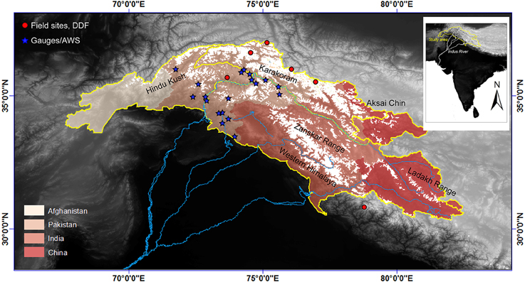
Figure 1. Location of glaciated portion of the upper Indus River watershed (in white) and key mountain ranges. Indus watershed as defined by Global Runoff Data Center. Also noted are the locations of all publicly available meteorological stations and streamflow data in the region (blue stars), and those glaciers where degree-day melt factors have been measured (red dots).

TABLE 1

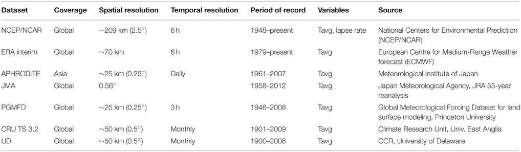
Table 1. Overview of the gridded reanalysis climate datasets compared in this study.

For the purpose of comparison, we use monthly average temperatures from each of the seven datasets for the period of common overlap, 1979–2007, and used them to derive the gridded climatological monthly means that we then used to implement our positive degree-day (PDD) melt model.

Glacier Area

Recent estimates of glacierized area in the Himalayas range between 33,000 and 60,000 km², with more than 23,000 glaciers (Dyurgerov and Meier, 2005; Zemp et al., 2009; Bolch et al., 2012; Kääb et al., 2012; Yao et al., 2012). To capture the fullest extent of the glaciers in the Indus watershed, we used the most recent version of the Randolph Glacier Inventory (RGI 4.0) (Pfeffer et al., 2014). The RGI incorporates both current and historical data to accurately approximate global glacier coverage. The database has extensive coverage and compiles a number of databases into one. While this greatly simplifies analysis, the inventory has the explicit drawback of inconsistency in sampling time periods, which results in significant uncertainty in estimates of glacier extent in regions where recent glacier change is significant. That said, the RGI inventory is widely used in the region. Other recently developed glacier inventories for HMA in particular, such as the ICIMOD and GAMDAM inventories (Bajracharya and Shrestha, 2011; Nuimura et al., 2014) have not yet been widely used or verified, hence we use the RGI 4.0 here in order to avoid introducing further uncertainty.

We define the Indus hydrologic watershed by the Global Runoff Database (World Meteorological Organization, 2014). There are 20,279 individual glaciers in the RGI 4.0 within the watershed so defined. Each glacier is represented by a single latitude and longitude centroid coordinate, maximum, minimum and mean elevation, glacier surface area, orientation, and length. The glacier area and area accuracy, and the date of the image used to identify glacier areas, are also available for a subset of the glaciers in the RGI inventory (see http://glims.org/RGI).

We find a total glaciated surface area of 29,413 km² in the Indus watershed, approximately 12% of the total upper basin area of 220,000 km² (Yu et al., 2013) (see Figure 1). The average elevation of the 20,279 glaciers is 5243 ± 547 m.a.s.l., with a range of mean elevation from ~2975 to 7200 m.a.s.l. (Figure 2A). The estimated mean elevation of the late summer snowline is 5000 m.a.s.l. Most of the glaciers below 5000 m.a.s.l. are in the Hindu Kush and Karakoram in the northwest of Afghanistan and Pakistan, and some are located at lower elevations and northern aspects of the High Himalaya in India. Median glacier size is 1.4 km². The vast majority (97%) of glaciers have surface areas of less than 5 km²; however, 46 glaciers cover areas larger than 100 km². Most of the glaciers larger than 5 km² are in the Karakoram (Figure 2B).

FIGURE 2

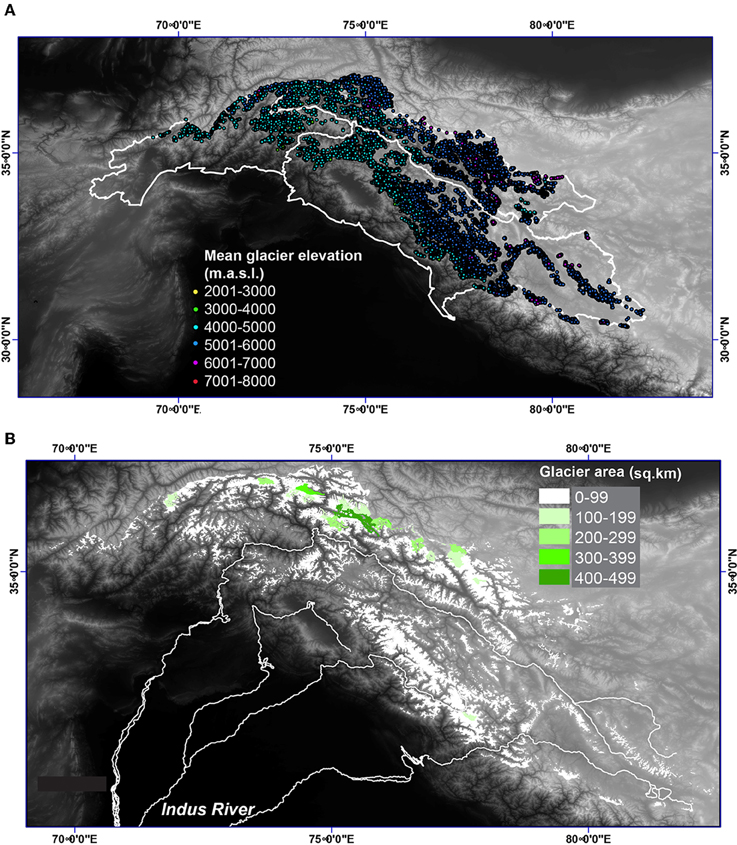
Figure 2. (A) Spatial distribution of mean glacier elevation (in meters above sea level). (B) spatial distribution of glacier size (surface area, in km²) across the Indus watershed.

Positive Degree-day Model for Meltwater Flux

In order to calculate the mean annual glacier meltwater flux to the Indus watershed over the past 40 years, we found the melt rate for each glacier with a PDD temperature-index melt model (Ambach and Kuhn, 1985; Braithwaite, 1995; Hock, 2003; Bliss et al., 2014; Radic and Hock, 2014). Temperature-index models rely on the premise that surface air temperature, one of the more accurate variables available from most climate datasets, is proportional to the mass loss from glaciers over time (Oerlemans, 2005; Cuffey and Paterson, 2010). In particular, the PDD approach assumes melt is proportional to the per-day-sum of all temperatures greater than the melting point (the degree days). The proportionality constant relating melt to the PDDs, i.e., the melt factor, depends on the glacier surface albedo, which is a function of both latitude and the conditions at the glacier surface, such as debris-cover, clean ice or fresh snow (e.g., Braithwaite, 1995; Kayastha et al., 2003; Collier et al., 2015). Unlike more complex and data-intensive mass and energy balance models, degree-day models are simple to implement: the only components necessary to run the model are the glacier surface area and elevation, the temperature at the glacier surface, and a melt factor (Ambach and Kuhn, 1985; Braithwaite, 1995; Rupper et al., 2009). The main limitation to this modeling approach is that they do not take into account spatial and temporal changes in factors such as precipitation, cloudiness or debris-cover that may influence albedo.

While an energy-balance approach would be more physically based, observational and modeled data for surface energy flux and mass balance gradients for individual glaciers is highly limited in the region (see Figure 1). The study area is large, with large variations in glacier area, aspect, hypsometry, debris cover and spatial and temporal precipitation distribution; hence, an energy and mass balance approach would be computationally intensive and attended by significant uncertainties. There is also a dearth of both weather stations and climate models at high enough resolution to provide the surface energy inputs and mass balance gradients necessary to implement an accurate energy balance modeling approach to quantify melt for individual glaciers across the region. Moreover, unlike for precipitation rates (e.g., Palazzi et al., 2013), surface temperature is one of the more certain outputs in all of the climate datasets available for this region. Additionally, a number of reports suggest that changes in glacier areas in the HMA are driven primarily by temperature (Ambach and Kuhn, 1985; Braithwaite, 1995; Kayastha et al., 1999; Rupper et al., 2009, 2012). A PDD/temperature index approach is therefore appropriate for this large region.

Total annual per-glacier meltwater flux is estimated from the mean elevation of each glacier, the 2 m air temperature at that elevation, a regional temperature lapse rate, a melt factor, and the glacier surface area (see Figure 3).

FIGURE 3

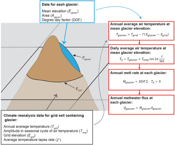
Figure 3. Schematic illustration of the data inputs and calculations used to derive the final meltwater flux at each glacier. The gray, background grids illustrate a coarse reanalysis grid. The cartoon mountain with a blue glacier illustrates the location of the glacier relative to these reanalysis grids. The gray and blue boxes contain a list of the data required as input into the series of equations used to calculate meltwater flux (outlined in red boxes).

The annual average air temperature at each glacier (see Figure 4) is determined as:

$\begin{array}{cc}{T}_{glacier}=T_{grid}+\Gamma \left(E_{glacier}-E_{grid}\right)& \left(1\right)\end{array}$

where T_grid (in °C) is the above-ground gridded temperature of the grid cell in which the glacier is located, Γ (in °C m⁻¹) is the adiabatic temperature lapse rate from the NCEP/NCAR Reanalysis dataset (Kalnay et al., 1996), E_glacier (in m.a.s.l.) is the mean elevation of the glacier, and E_grid (in m.a.s.l.) is the gridded elevation of the climate data cell in which the glacier is located.

FIGURE 4

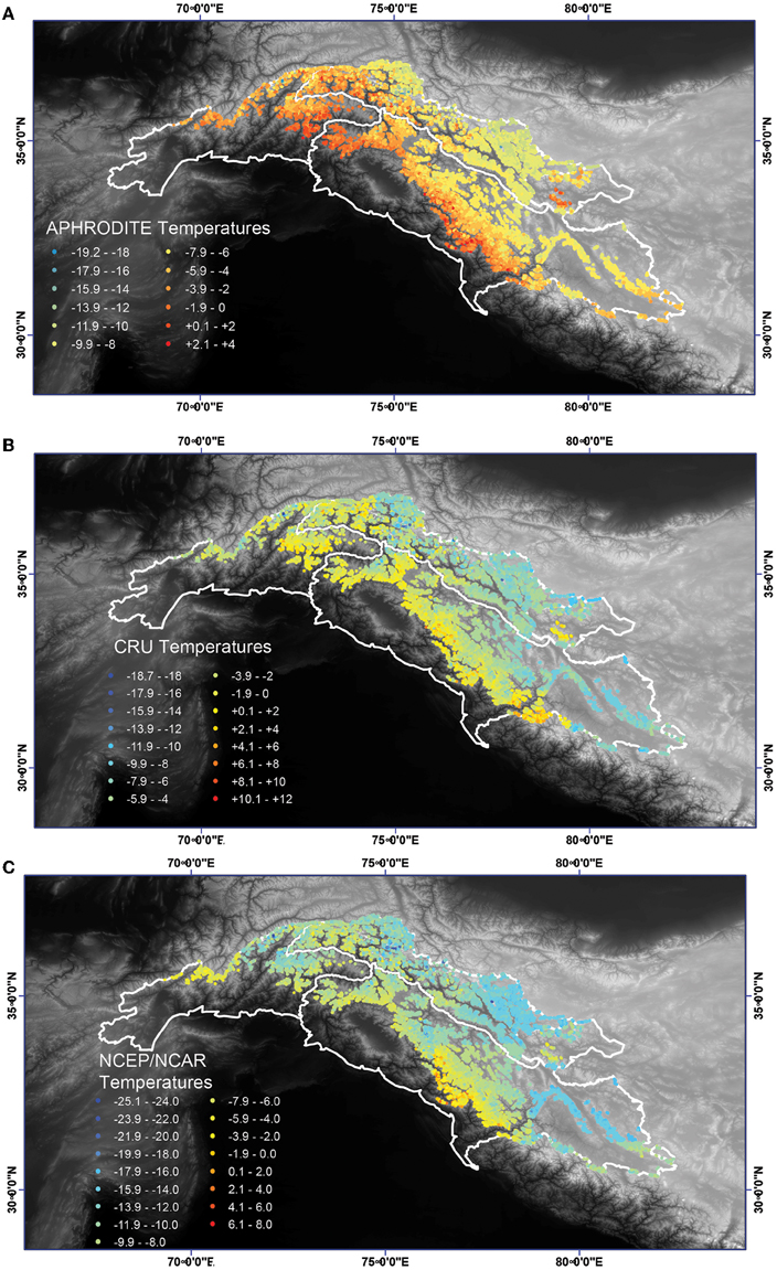
Figure 4. Distribution of mean annual glacier 2 m air temperatures (in °C) at the mean glacier elevation across the Indus watershed. (A) using the APHRODITE, (B) CRU, and (C) NCEP temperature data. Note the temperature color scale varies for each dataset.

We calculate the positive degree days (PDDs) using monthly reanalysis output by calculating daily mean air temperature (T_a) as:

$\begin{array}{cc}{T}_a=T_{glacier}+T_{amp}\cos 2\pi \frac{t}{365}& \left(2\right)\end{array}$

where T_amp is the amplitude in the seasonal cycle in air temperature and t is the day of the year. The PDDs are then the sum of all daily temperatures greater than zero (Equation 3). Monthly data are used as not all reanalysis products provide daily data over the full period of interest.

The mean annual melt rate per glacier is:

$\begin{array}{cc}{M}_{glacier}=DDF{\displaystyle \sum T_a>0},& \left(3\right)\end{array}$

where M_glacier is total annual melt (meters of water equivalent per year), T_a is daily mean air temperature at the glacier surface (°C), and DDF is the melt factor relating snow and ice melt to surface air temperature (mm d⁻¹ °C⁻¹), which depends on the conditions at the glacier surface. We set fresh snow to 4 m yr⁻¹ °C⁻¹, clean ice to 6.5 m yr⁻¹ °C⁻¹, and dirty ice to 9 m yr⁻¹ °C⁻¹ following Cuffey and Paterson (2010), Shea et al. (2009), and Zhang et al. (2006). These melt factors compare favorably with the few empirically-derived melt factors from across HMA (see Figure 1): the mean observed melt factor in HMA is 8 ± 3.4 mm d⁻¹ °C⁻¹, the minimum (snow) is 3.7 mm d⁻¹ °C⁻¹ and the maximum (dirty ice) is 13.8 mm d⁻¹ °C⁻¹ (Kayastha et al., 2000, 2003; Singh et al., 2000; Zhang et al., 2006). We note that all empirically-derived melt factors were measured over a limited summer season of at most 3 months (Hock, 2003). While debris thickness is presumed to influence melt rates (Scherler et al., 2011) by enhancing melt with thin debris cover and impeding melt as it thickens, recent studies indicate that debris-covered ice in the region has thinned at a rate similar to that of exposed clean ice (Bolch et al., 2012; Kääb et al., 2012; Collier et al., 2015). Hence, we implement a single average melt factor, derived from measurements on clean ice as a first-order approximation of ice melt across the region.

The meltwater flux (Q_glacier), assuming melt (and runoff) rate (M_glacier) from each individual glacier is the product of the total annual melt and the glacier surface area [A_glacier (in m²)] over which melt is occurring, is:

$\begin{array}{cc}{Q}_{glacier}=M_{glacier}{A}_{glacier}& \left(4\right)\end{array}$

The total annual meltwater contribution to the Indus watershed is the sum of all individual glacier meltwater fluxes. Hence, uncertainty will arise from uncertainty in the climate data used (T_grid and T_glacier), estimates of glacier area and elevation (A_glacier and E_glacier), the melt factor (DDF) and lapse rate (Γ).

Model Parameterizations

Model parameterization necessarily introduces additional uncertainty in the melt calculations. In order to bound our modeled meltwater flux within a plausible range, we used sets of input parameters that may reasonably be said to represent the mean, maximum, and minimum melt scenarios in the Upper Indus watershed, respectively: (a) mean monthly two meter air temperature, the mean of the empirically-derived melt factors across High Mountain Asia (6.5 mm d⁻¹ C⁻¹) and a melting surface area of 75% (after Cuffey and Paterson, 2010), (b) adiabatic lapse rate reduced by 1°C km⁻¹, the maximum empirically-derived melt factor for the region that is appropriate for dirty ice (9.0 mm d⁻¹ C⁻¹), and a melting surface area of 100%, and (c) an adiabatic lapse rate increased by 1°C km⁻¹, the minimum empirically-derived melt factor that would be appropriate for snow (4.0 mm d⁻¹ C⁻¹), and a melting surface area of 45% (the ablation area) (see Table 2).

TABLE 2

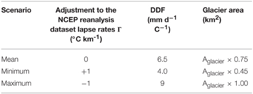
Table 2. Summary of parameters used in the degree-day model to find upper and lower bounds and mean meltwater flux.

The maximum and minimum parameterizations should be viewed as extreme endmembers, providing wide bounds to potential meltwater flux in the study area. This method allowed us to highlight spatial trends and variability in glacier meltwater runoff and assess the relative importance of the lapse rate, temperature, melt factor, and glacier surface area to the total uncertainty in our calculated meltwater volumes.

Analysis of Results

Spatial Distribution of Meltwater Flux and Temperature

Glacier meltwater flux integrated over the study area for each climate dataset is in Figure 5 and the spatial distribution of the mean annual meltwater flux by glacier (in km³ yr⁻¹) is in Figure 6. The results vary significantly between the climate datasets, from an integrated meltwater flux of 8–169 km³ yr⁻¹, with NCEP/NCAR and APHRODITE temperature data representing the endmembers (see Figure 5). The average meltwater contribution across all climate datasets for the 1979–2007 was 90 km³ yr⁻¹, or 41% of total mean annual runoff (Table 3). All model inputs except temperature were held constant (by design), hence differences in the meltwater flux estimates are solely the result of differences in the gridded temperature datasets.

FIGURE 5

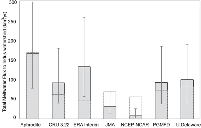
Figure 5. Comparison of watershed-integrated meltwater flux across the Indus watershed for seven climate datasets. The error bars illustrate the extreme minimum and maximum meltwater flux assuming systematic parametrization of the degree-day model. The dashed lines are the integrated meltwater fluxes if temperatures for all datasets are adjusted to the same mean temperature.

FIGURE 6

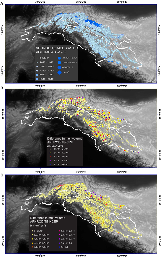
Figure 6. (A) Distribution of mean annual meltwater flux by glacier across the Indus watershed. The meltwater fluxes were calculated using APHRODITE temperature dataset as control. (B) Difference in melt volume generated between APHRODITE and CRU temperature datasets. (C) Difference in melt volume generated between APHRODITE and NCEP datasets. Meltwater volumes are in km³/yr.

TABLE 3

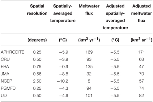
Table 3. Climate dataset, spatial resolution, 2 m air temperature averaged across all glaciers, integrated meltwater flux for the Indus watershed, integrated meltwater flux for the Indus watershed when all temperatures are adjusted to the same mean.

Closer inspection of the spatial pattern in temperatures at the glacier elevations, using the APHRODITE temperature dataset as control, provides important insights into some of the key differences between the reanalysis datasets. The spatial distribution of glaciers with mean annual surface temperatures >0°C (above freezing) were found throughout the watershed in every country except Afghanistan (Figure 4). Temperatures at the mean elevation of the glaciers ranged between −20.0 and 10.5°C, with a mean of −5.9°C (Figure 7B).

FIGURE 7

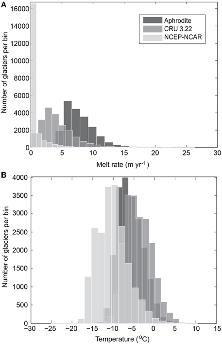
Figure 7. Histograms of (A) glacier melt rate and (B) temperature for three climate datasets: APHRODITE (dark gray), CRU (intermediate gray), and NCEP (lightest gray). Note that all three melt-rate histograms are right-skewed while temperatures show a Gaussian distribution. As temperatures decrease, the median melt rates shift to lower values, resulting in an increasing number of glaciers binned into the zero melt rate (as seen with NCEP here). This leads to a significant number of glaciers not contributing to the total meltwater flux when using NCEP temperature data as compared to APHRODITE and CRU.

On average, the glacier surface temperatures derived using the CRU dataset are 2°C warmer than those found using the APHRODITE temperature data, but the spatial pattern is very similar (spatial correlation coefficient equal to 0.82). One distinct exception is in the southernmost edge of the watershed on the northern aspects of the Garwhal Himalaya of India, where temperatures using APHRODITE are more than 4°C warmer than CRU, perhaps reflecting the incorporation of orographic effects in higher spatial resolution climate reanalysis data.

The NCEP/NCAR reanalysis temperatures are also spatially correlated with both APHRODITE and CRU (correlation coefficients of 0.86 and 0.74, respectively (see Table 4). However, NCEP/NCAR temperatures are significantly cooler than temperatures from the other datasets, ranging from −24 to +8°C, with a spatially-averaged glacier temperature of −10.2°C (Table 3). Temperature derived from the remaining datasets varies within the range of those from the APHRODITE and NCEP/NCAR reanalyses.

TABLE 4

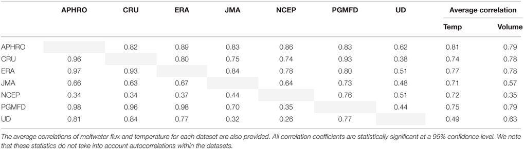
Table 4. Spatial correlations of air temperature at the glaciers (right of gray diagonal) and of meltwater flux (left of gray diagonal) between climate datasets.

Despite some notable spatial differences in temperatures between reanalysis dataset, the spatial distribution is highly and significantly correlated (p-value < 0.005) (Table 4)—that is, the pattern of temperature variation across the study area correlates between datasets even when absolute temperatures do not. (The one exception is the UD dataset. The spatial correlations between UD and the other datasets are statistically significant, but the correlations are not very high.) Therefore, the primary driver of the large spread in meltwater flux is the difference in spatially-averaged, or baseline, temperatures (Table 3). This is because temperatures can be negative while melt cannot and the datasets with lower baseline temperatures will have a greater number of glaciers with zero melt. This is illustrated in Figure 7 which shows that the values for temperature within the datasets approximate a Gaussian distribution while the distribution of meltwater flux is right-skewed. In particular, NCEP and JMA have much lower average temperatures than the other datasets, low enough that many glaciers produce minimal or no meltwater thereby decreasing the spatial correlation between meltwater fluxes (Table 4) and driving their integrated meltwater fluxes much lower than the other datasets (Table 3).

To better compare the pattern of meltwater flux variability between temperature datasets (rather than absolute values) we applied systematic adjustment to each to standardize the spatially-averaged temperature. The result was an increase in the spatial correlation of meltwater flux between temperature datasets. Most notably, the average spatial correlation between NCEP/NCAR meltwater flux with the other datasets increases from 0.35 to 0.71, and the average correlation between JMA meltwater flux with the other datasets increases from 0.57 to 0.69. We are able to conclude that a significant proportion (~70%) of the differences in watershed-integrated meltwater flux is driven by the differences in spatially-averaged temperature between the datasets. The remaining proportion of the integrated meltwater flux differences (Table 3 and Figure 5) is the result of spatial differences in temperatures from one dataset to the other.

Interestingly, the spatial resolution of the climate input data is not necessarily a good predictor of the magnitude of the integrated meltwater flux (see Table 3). While APHRODITE, the dataset with the highest spatial resolution, produced the greatest estimate of total meltwater flux in the Indus watershed, and NCEP, with the lowest spatial resolution, produces the lowest estimate, the remainder of the datasets did not follow any particular pattern.

Spatial Distribution of Meltwater Flux and Glacier Size

For each dataset, the spatial correlation of meltwater flux with glacier area is significantly higher than the spatial correlation of meltwater flux with temperature (Table 5, Figure 8). This is due to the role glacier size plays in meltwater flux. Larger glaciers tend to have higher meltwater fluxes, and thus the spatial pattern in glacier size (which is the same for regardless of the climate dataset used) increases the meltwater flux correlations for each climate dataset. In other words, the size of each glacier is a much better predictor of meltwater flux than temperature (and hence melt rate) at the glacier surface (Table 5, Figure 8). For the Indus watershed, the largest meltwater fluxes were found in the Karakoram and High Himalaya of India, where the largest glaciers are (Figure 6). This result is robust across all climate datasets, with the possible exception of NCEP, wherein temperature estimates tended to be well below the 0°C isotherm, and hence many glaciers produced little to no melt (See Figure 7). The uncertainty in glacier area and change in glacier area over time will therefore lead to significant uncertainty in regional meltwater flux calculations and projections.

TABLE 5

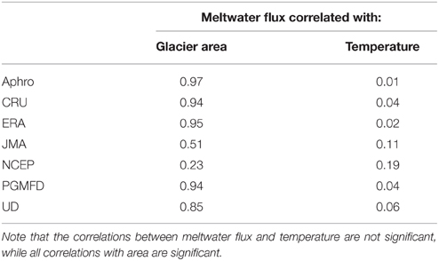
Table 5. Spatial correlation of meltwater flux with glacier area and mean 2 m air temperature at the glacier.

FIGURE 8

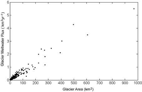
Figure 8. Comparison of glacier area and meltwater flux for all glaciers using the APHRODITE climate data. Note the significant correlation between glacier area and flux. This is similar for all datasets, but with varying slopes.

Meltwater Flux and Parameter Uncertainties

Beyond temperature, uncertainties in glacier area over which melt is assumed to occur, environmental lapse rate, and complexities that influence melt factors (e.g., debris-cover, avalanching onto glacier surfaces, deposition of black carbon) will also give rise to uncertainty in the meltwater fluxes. The minimum and maximum melt model scenarios provide bounds on the meltwater contribution and highlight how the meltwater fluxes may vary due to large uncertainties in these input parameters (Figure 5).

Using the APHRODITE dataset as control and the three model parameterizations, annual meltwater contributions to the Indus River over the period 1979–2007 ranged from a minimum of 79 km³ yr⁻¹ to a maximum of 302 km³ yr⁻¹ and averaged 169 km³ yr⁻¹. Given total runoff in the Indus River has averaged 218 km³ yr⁻¹ during this period (Sharif et al., 2012; Yu et al., 2013), the maximum bound on melt parameterization is clearly unrealistic. By contrast, the CRU climate data produced a lower estimate of meltwater flux of between 40 and 181 km³ yr⁻¹ with an average of 93 km³ yr⁻¹. At the lowest end of the range of estimated meltwater flux, the NCEP/NCAR climate data resulted in annual melt volumes of between 2 and 26 km³ yr⁻¹, with an average of 8 km³ yr⁻¹. These are extreme melt model scenarios, but highlight the fact that the choice of climate dataset will give rise to uncertainties of the same order of magnitude as the largest, systematic uncertainties in all model parameters.

Key Regions of Meltwater Contribution

Given the high spatial correlation between glacier meltwater fluxes between climate dataset, we considered it robust to evaluate which glaciers contribute the most meltwater runoff and whether they share common characteristics. Overall, variations in the spatial patterns of glacier elevation, glacier surface area, and surface temperatures provide an a priori control on spatial patterns in meltwater flux across the watershed. As expected, given that most of the largest and lowest elevation glaciers are located in the Karakoram and Hindu Kush ranges of Pakistan, and a large percentage of the total glaciated area in the Indus is located in Pakistan, the glaciated mountain ranges of Pakistan contribute the largest meltwater flux of all the countries in the Indus watershed, in all cases.

Importantly, we find that despite differences in estimates of glacier runoff between the climate datasets, most of the meltwater comes from a small percentage of the glaciers (Figure 9). This result is robust across all datasets and is independent of the modeling assumptions. Less than 1% of the glaciers in the Upper Indus basin contribute half of the total meltwater runoff to the Indus River, and, 10% of them more than 80% of total glacier runoff (Figure 9). Most of these glaciers are in the Hindu Kush and Karakoram of Pakistan, but a few large glaciers are in the High Himalaya of Himachal Pradesh and the Aksai Chin of China (Figure 6). Given their outsized impact on water resources in the Indus Basin, we suggest that these glaciers should be the target of further detailed research, and fieldwork in particular.

FIGURE 9

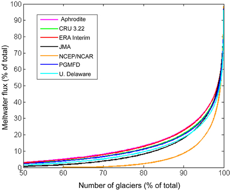
Figure 9. Percentage of glaciers in the Indus watershed contributing to the total glacial melt flux. Regardless of dataset used, less than 1% of the glaciers contribute over 50% of the meltwater, and 10% contribute over 80% of the total meltwater to annual runoff.

Changes in Meltwater Flux with Regional Climate Change

To test the sensitivity of glacier meltwater flux in the Upper Indus watershed to current and future climate change, we calculated the change in flux under a range of temperature projections generated for the IPCC AR5. The 5th phase of the IPCC Climate Model Intercomparison Project project warming across HMA by 2100 AD, from 1.8 ± 0.5°C (RCP 4.5) to 3.7 ± 0.7°C (RCP 8.5) (Collins et al., 2013). Most future warming scenarios project at least 1°C warming across HMA in the next 50 years (Christensen et al., 2007).

We ran our mean model parameterization with mean temperature from all seven climate reanalysis datasets as the baseline and forced it with regional warming scenarios of 2 and 4°C (Cruz et al., 2007). For each model run, warming was applied equally across the study area. We assume that the surface area of all glaciers in the Indus watershed continue to shrink at the same rate of 0.1–0.4% per year that they have exhibited over the last 50 years (Bolch et al., 2012), and use the reduced glacier area and warming scenarios to calculate the percent change in total annual metlwater flux by 2100 AD (Figure 10).

FIGURE 10

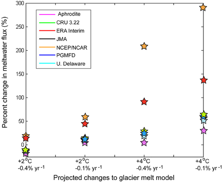
Figure 10. Projected percentage change in meltwater flux, relative to the mean meltwater flux for the 1979–2007 period, assuming warming of 2–4°C by 2100 AD (IPCC, 2013), and a constant rate of glacier area decrease of 0.1–0.4% yr⁻¹ (i.e., 6–26% reduction in glacier extents by 2100 AD) (Bolch et al., 2012).

We find a very large spread in the response of meltwater flux from −10 to +10% with 2°C warming and 0.1% per year area reduction, to +30 to +290% volume with 4°C warming and 0.4% per year area reduction. These results should be viewed with caution due to the simplicity of our approach; nevertheless, our findings highlight the dependence of future climate impact projections on the climate dataset that is used, and the fact that the spread in meltwater flux estimates between climate datasets becomes larger as the imposed temperature change (RCP scenario) increases (Figure 10).

Ours is a conservative estimate of the change in meltwater contribution, as we have assumed an average melt rate over the entire glacier surface, while in reality the highest melt rates occur in the lowest reaches of the glaciers that are typically the areas being lost during glacier shrinkage and retreat. However, we have not considered the unlikely but plausible scenario of glacier expansion, should precipitation rates increase sufficiently that enhanced melt due to a temperature increase is offset. Given that we find meltwater flux is highly sensitive to glacier surface area, this potential glacier response to climate change will be an important consideration in future analyses.

Conclusions

We applied a PDD melt model and a selection of gridded reanalysis climate datasets to the glaciers in the Indus River watershed to quantify the contribution of glacier meltwater runoff to total annual discharge. Our results, using a reasonable mean parameterization of melt factors for the region, range from 8 to 169 km³ yr⁻¹ for the period 1979–2007, depending on the temperature dataset chosen. This suggests glacier melt accounts for on average between 4 and 77% of the average annual discharge of the Indus, dependent upon the baseline climate dataset chosen. When applying extreme minimum and maximum bounds in the melt model parameters for each climate dataset, we find a similar range of variability in melt estimates. Thus, the uncertainty inherent in climate reanalysis datasets represents a significant challenge to quantification and projection of glacier changes across large regions such as HMA. Even when any uncertainty derived from estimates of glacier surface area and melt factors are minimized, there remains significant uncertainty propagated by the necessary use of climate reanalysis datasets to drive glacio-hydrological models, that must be acknowledged in any use of these data for modeling purposes. This is an issue not only when using gridded climate data, as we have done, but also when using sparse weather station data that is extrapolated to disparate glaciated areas in this remote and high relief region.

We have demonstrated that estimates of modeled glacier runoff in the Indus Basin vary by more than an order of magnitude between reanalysis datasets, but found also that the spatial pattern of melt across the study region is robust and independent of both the temperature datasets and the model parameterization. Indeed, the spatial correlation of meltwater volumes between the climate datasets, with the exception of NCEP and JMA, is r ~ 0.79. We are therefore able to conclude that fewer than 10% of the glaciers in the watershed contribute more than 80% of the total meltwater flux to the Indus River. Meltwater runoff is greatest where glaciers occupy relatively low elevations and large surface areas. The vast majority of these are in the Hindu Kush-Karakoram, and fewer in the Himachal Pradesh, India. Our results show that the largest glaciers in the Karakoram are particularly important to runoff in the Indus River. Focused research on these glacier are critical to more accurately project the impact of changing glacier-hydrology on downstream transboundary water resources in the Indus drainage basin.

Given that glacier surface area has a significant influence on any melt volume calculations, over time changes in glacier size will impact meltwater production to a similar extent as any projected regional change in temperature (or precipitation). Continued focus is hence needed to more accurately represent both the total number of glaciers in the Indus watershed and any spatial variability in glacier area and length changes, as well as better quantification of regional temperature and precipitation changes across the wider Himalayan region, in order to assess the meltwater response to ongoing regional climate change.

Our climate sensitivity analysis suggests that infrastructure and development in the Indus watershed over the past few decades has been predicated upon higher than normal meltwater volumes, as temperatures have increased faster than glaciers have responded by thinning and shrinking. Dependent upon the baseline climate chosen, glacier meltwater contributions will increase slightly to significantly in the coming century, but will likely ultimately decrease as the total glacierized area in the watershed continues to decrease. Uncertainties in our parametrizations of melt leads to additional uncertainty in the projections of future glacier extent, and has roughly the same importance as the uncertainty in both the baseline climate data and in the climate projections. Much of this glacier response to climate change will be ultimately controlled by a few key glaciers in the Karakoram and High Himalaya. In order to more accurately predict current and future glacier meltwater contributions to all of the major rivers of the Himalayan region, future efforts should focus on minimizing uncertainties in the global climate datasets used, in the melt models applied and, more importantly, in more accurately measuring past and present glacier area changes.

Conflict of Interest Statement

The authors declare that the research was conducted in the absence of any commercial or financial relationships that could be construed as a potential conflict of interest.

Acknowledgments

Funding for this project was provided in part by a Brigham Young University mentoring grant and an NSF grant (#1304397) to SR, and a Natural Sciences and Engineering Research Council (NSERC) operating grant to MK. We thank G. Cogley, T. Bolch and two anonymous reviewers for suggestions on an earlier version of this manuscript.

References

Ambach, W., and Kuhn, M. (1985). Accumulation gradients in Greenland and mass balance response to climatic changes. Z. Gletscherkd Glazialgeol. 21, 311–317.

Barnett, T. P., Adam, J. C., and Lettenmaier, D. P. (2005). Potential impacts of a warming climate on water availability in snow-dominated regions. Nature 438, 303–309. doi: 10.1038/nature04141

PubMed Abstract | CrossRef Full Text | Google Scholar

Bajracharya, S. R., and Shrestha, B. (eds.). (2011). The Status of Glaciers in the Hindu Kush-Himalayan Region. Kathmandu: ICIMOD.

Google Scholar

Bliss, A., Hock, R., and Radic, V. (2014). Global response of glacier runoff to twenty-first century climate change. J. Geophys. Res. Earth Surf. 119, 717–730. doi: 10.1002/2013jf002931

CrossRef Full Text | Google Scholar

Bolch, T., Kulkarni, A., Kääb, A., Huggel, C., Paul, F., Cogley, J. G., et al. (2012). The state and fate of Himalayan glaciers. Science 336, 310–314. doi: 10.1126/science.1215828

PubMed Abstract | CrossRef Full Text | Google Scholar

Bookhagen, B., and Burbank, D. W. (2010). Toward a complete Himalayan hydrological budget: spatiotemporal distribution of snowmelt and rainfall and their impact on river discharge. J. Geophys. Res. Earth Surf. 115:F03019. doi: 10.1029/2009JF001426

CrossRef Full Text | Google Scholar

Braithwaite, R. J. (1995). Positive degree-day factors for ablation on the Greenland ice-sheet studied by energy-balance modeling. J. Glaciol. 41, 153–160.

Google Scholar

Christensen, J. H., Hewitson, B., Busuioc, A., Chen, A., Gao, X., Held, I., et al. (2007). “Regional climate projections, in climate change 2007: the physical science basis,” in Contribution of Working Group 1 to the 4th Assessment Report of the Intergovernmental Panel on Climate Change, eds S. Solomon, D. Qin, M. Manning, Z. Chen, M. Marquis, K. B. Averyt, M. Tignor, and H. L. Miller (Cambridge; New York, NY: Cambridge University Press), 847–940.

Collier, E., Maussion, F., Nicholson, L. I., Mölg, T., Immerzeel, W. W., and Bush, A. B. G. (2015). Impact of debris cover on glacier ablation and atmosphere-glacier feedbacks in the Karakoram. Cryosphere Discuss. 9, 2259–2299. doi: 10.5194/tcd-9-2259-2015

CrossRef Full Text | Google Scholar

Collins, M., Knutti, R., and Arblaster, J. (2013). “Long-term climate change: projections, commitments and irreversibility [M/OL],” in Climate Change 2013: The Physical Science Basis. Contribution of Working Group I to the Fifth Assessment Report of the Intergovernmental Panel on Climate Change, eds S. Joussaume, A. Mokssit, K. Taylor, and S. Tett (Cambridge; New York, NY: Cambridge University Press), 1031–1106.

Cook, E. R., Palmer, J. G., Ahmed, M., Woodhouse, C. A., Fenwick, P., Zafar, M. U., et al. (2013). Five centuries of Upper Indus River flow from tree rings. J. Hydrol. 486, 365–375. doi: 10.1016/j.jhydrol.2013.02.004

CrossRef Full Text | Google Scholar

Cruz, R. V., Harasawa, H., Lal, M., Wu, S., Anokhin, Y., Punsalmaa, B., et al. (2007). “Asia, in climate change 2007: impacts, adaptation and vulnerability,” in Contribution of Working Group II to the Fourth Assessment Report of the Intergovernmental Panel on Climate Change, eds M. L. Parry, O. F. Canziani, J. P. Palutikof, P. J. van der Linden, and C. E. Hanson (Cambridge: Cambridge University Press), 471–490.

Cuffey, K. M., and Paterson, W. S. B. (2010). Physics of Glaciers, 4th Edn. Amsterdam: Elsevier, Inc.

Google Scholar

Dee, D. P., Uppala, S. M., Simmons, A. J., Berrisford, P., Poli, P., Kobayashi, S., et al. (2011). The ERA−Interim reanalysis: configuration and performance of the data assimilation system. Q. J. R. Meteorol. Soc. 137, 553–597. doi: 10.1002/qj.828

CrossRef Full Text | Google Scholar

Dyurgerov, M. D., and Meier, M. F. (2005). Glaciers and the Changing Earth System: A 2004 Snapshot. Institute of Arctic and Alpine Research, University of Colorado.

Fan, Y., and Van den Dool, H. (2008). A global monthly land surface air temperature analysis for 1948–present. J. Geophys. Res. Atmospheres 113:D01103. doi: 10.1029/2007JD008470

CrossRef Full Text | Google Scholar

Harris, I., Jones, P. D., Osborn, T. J., and Lister, D. H. (2014). Updated high−resolution grids of monthly climatic observations–the CRU TS3. 10 Dataset. Int. J. Climatol. 34, 623–642. doi: 10.1002/joc.3711

CrossRef Full Text | Google Scholar

Hock, R. (2003). Temperature index melt modeling in mountain areas. J. Hydrol. 282, 104–115. doi: 10.1016/S0022-1694(03)00257-9

CrossRef Full Text | Google Scholar

Immerzeel, W. W., Pellicciotti, F., and Bierkens, M. F. P. (2013). Rising river flows throughout the twenty-first century in two Himalayan glacierized watersheds. Nat. Geosci. 6, 742–745. doi: 10.1038/ngeo1896

CrossRef Full Text | Google Scholar

Immerzeel, W. W., Van Beek, L. P. H., and Bierkens, M. F. P. (2010). Climate change will affect the Asian water towers. Science 328, 1382–1385. doi: 10.1126/science.1183188

PubMed Abstract | CrossRef Full Text | Google Scholar

IPCC. (2013). “Annex II: climate system scenario tables,” in Climate Change 2013: The Physical Science Basis, eds M. Prather, G. Flato, P. Friedlingstein, C. Jones, J.-F. Lamarque, H. Liao and P. Rasch, in Contribution of Working Group I to the Fifth Assessment Report of the Intergovernmental Panel on Climate Change, eds T. F. Stocker, D. Qin, G.-K. Plattner, M. Tignor, S. K. Allen, J. Boschung et al. (Cambridge; New York, NY: Cambridge University Press), 1395–1445.

Jianchu, X., Shrestha, A., Vaidya, R., Eriksson, M., and Hewitt, K. (2007). The Melting Himalayas: Regional Challenges and Local Impacts of Climate Change on Mountain Ecosystems and Livelihoods. Kathmandu: International Centre for Integrated Mountain Development.

Google Scholar

Kääb, A., Berthier, E., Nuth, C., Gardelle, J., and Arnaud, Y. (2012). Contrasting patterns of early twenty-first-century glacier mass change in the Himalayas. Nature 488, 495–498. doi: 10.1038/nature11324

PubMed Abstract | CrossRef Full Text | Google Scholar

Kalnay, E., Kanamitsu, M., Kistler, R., Collins, W., Deaven, D., Gandin, L., et al. (1996). The NCEP/NCAR 40-year reanalysis project. Bull. Am. Meteorol. Soc. 77, 437–471.

Google Scholar

Kaser, G., Grohauser, M., and Marzeion, B. (2010). Contribution potential of glaciers to water availability in different climate regimes. Proc. Natl. Acad. Sci. U.S.A. 107, 20223–20227. doi: 10.1073/pnas.1008162107

PubMed Abstract | CrossRef Full Text | Google Scholar

Kayastha, R. B., Ageta, Y., and Nakawo, M. (2000). Positive degree-day factors for ablation on glaciers in the Nepalese Himalayas: case study on Glacier AX010 in Shorong Himal, Nepal. Bull. Glaciol. Res. 17, 1–10.

Google Scholar

Kayastha, R. B., Ageta, Y., Nakawo, M., Fujita, K., Sakai, A., and Matsuda, Y. (2003). Positive degree-day factors for ice ablation on four glaciers in the Nepalese Himalayas and Qinghai-Tibetan Plateau. Bull. Glaciol. Res. 20, 7–14.

Kayastha, R. B., Ohata, T., and Ageta, Y. (1999). Application of a mass-balance model to a Himalayan glacier. J. Glaciology 45, 559–567.

Google Scholar

Khalid, S., Qasim, M., and Farhan, D. (2013). Hydro-meteorological characteristics of Indus River Basin at extreme north of Pakistan. J. Earth Sci. Clim. Change 5, 2. doi: 10.4172/2157-7617.1000170

CrossRef Full Text | Google Scholar

Kistler, R., Kalnay, E., Collins, W., Saha, S., White, G., Woollen, J., et al. (2001). The NCEP-NCAR 40-year reanalysis: monthly means CD-ROM and documentation. B. Am. Meteorol. Soc. 82, 247–267. doi: 10.1175/1520-0477(2001)082<0247:TNNYRM>2.3.CO;2

CrossRef Full Text | Google Scholar

Kobayashi, S., Ota, Y., Harada, Y., Ebita, A., Moriya, M., Onoda, H., et al. (2015). The JRA-55 reanalysis: general specifications and basic characteristics. J. Meteorol. Soc. Japan 2, 5–48. doi: 10.2151/jmsj.2015-001

CrossRef Full Text | Google Scholar

Kulkarni, A. V., Bahuguna, I. M., Rathore, B. P., Singh, S. K., Randhawa, S. S., Sood, R. K., et al. (2007). Glacial retreat in Himalaya using Indian remote sensing satellite data. Curr. Sci. 92, 69–74. doi: 10.1117/12.694004

CrossRef Full Text | Google Scholar

Lutz, A. F., Immerzeel, W. W., Gobiet, A., Pellicciotti, F., and Bierkens, M. F. P. (2013). Comparison of climate change signals in CMIP3 and CMIP5 multi-model ensembles and implications for Central Asian glaciers. Hydrol. Earth Syst. Sci. 17, 3661–3677. doi: 10.5194/hess-17-3661-2013

CrossRef Full Text | Google Scholar

Lutz, A. F., Immerzeel, W. W., Shrestha, A. B., and Bierkens, M. F. P. (2014). Consistent increase in High Asia's runoff due to increasing glacier melt and precipitation. Nat. Clim. Change 4, 587–592. doi: 10.1038/nclimate2237

CrossRef Full Text | Google Scholar

Mukhopadhyay, B., and Khan, A. (2014). A quantitative assessment of the genetic sources of the hydrologic flow regimes in Upper Indus Basin and its significance in a changing climate. J. Hydrol. 509, 549–572. doi: 10.1016/j.jhydrol.2013.11.059

CrossRef Full Text | Google Scholar

Nuimura, T., Sakai, A., Taniguchi, K., Nagai, H., Lamsal, D., Tsutaki, S., et al. (2014). The GAMDAM Glacier Inventory: a quality controlled inventory of Asian glaciers. Cryosphere Discuss. 8, 2799–2829. doi: 10.5194/tcd-8-2799-2014

CrossRef Full Text | Google Scholar

Oerlemans, J. (2005). Extracting a climate signal from 169 glacier records. Science 308, 675–677. doi: 10.1126/science.1107046

PubMed Abstract | CrossRef Full Text | Google Scholar

Palazzi, E., von Hardenburg, J., and Provenzale, A. (2013). Precipitation in the Hindu-Kush Karakoram Himalaya: observations and future scenarios. J. Geophys. Res. 118, 85–100. doi: 10.1029/2012JD018697

CrossRef Full Text | Google Scholar

Pellicciotti, F., Buergi, C., Immerzeel, W. W., Konz, M., and Shrestha, A. B. (2012). Challenges and uncertainties in hydrological modeling of remote Hindu Kush-Karakoram-Himalayan (HKH) basins: suggestions for calibration strategies. Mt. Res. Dev. 32, 39–50. doi: 10.1659/MRD-JOURNAL-D-11-00092.1

CrossRef Full Text | Google Scholar

Pfeffer, W. T., Arendt, A. A., Bliss, A., Bolch, T., Cogley, J. G., Gardner, A. S., et al. (2014). The Randolph Glacier Inventory: a globally complete inventory of glaciers. J. Glaciol. 60, 537–552. doi: 10.3189/2014JoG13J176

CrossRef Full Text | Google Scholar

Radic, V., and Hock, R. (2014). Glaciers in the earth's hydrological cycle: assessments of glacier mass and runoff changes on global and regional scales. Surv. Geophys. 35, 813–837. doi: 10.1007/s10712-013-9262-y

CrossRef Full Text | Google Scholar

Rupper, S., Roe, G., and Gillespie, A. (2009). Spatial patterns of Holocene glacier advance and retreat in Central Asia. Q. Res. 72, 337–346. doi: 10.1016/j.yqres.2009.03.007

CrossRef Full Text | Google Scholar

Rupper, S., Schaefer, S., Burgener, L., Koenig, L., Tsering, K., and Cook, E. (2012). Sensitivity and response of Bhutanese glaciers to atmospheric warming. Geophys. Res. Lett. 39:L19503. doi: 10.1029/2012GL053010

CrossRef Full Text | Google Scholar

Scherler, D., Bookhagen, B., and Strecker, M. R. (2011). Spatially variable response of Himalayan glaciers to climate change affected by debris cover. Nat. Geosci. 4, 156–159. doi: 10.1038/ngeo1068

CrossRef Full Text | Google Scholar

Sharif, M., Archer, D. R., Fowler, H. J., and Forsythe, N. (2012). Trends in timing and magnitude of flow in the Upper Indus Basin. Hydrol. Earth Syst. Sci. 9, 9931–9966. doi: 10.5194/hessd-9-9931-2012

CrossRef Full Text | Google Scholar

Shea, J. M., Moore, R. D., and Stahl, K. (2009). Derivation of melt factors from glacier mass-balance records in western Canada. J. Glaciology 55, 123–130. doi: 10.3189/002214309788608886

CrossRef Full Text | Google Scholar

Singh, P., Arora, M., and Goel, N. K. (2006). Effect of climate change on runoff of a glacierized Himalayan basin. Hydrol. Process. 20, 1979–1992. doi: 10.1002/hyp.5991

CrossRef Full Text | Google Scholar

Singh, P., Kumar, N., and Arora, M. (2000). Degree-day factors for snow and ice for Dokriani Glacier, Garhwal Himalayas. J. Hydrol. 235, 1–11. doi: 10.1016/S0022-1694(00)00249-3

CrossRef Full Text | Google Scholar

Thayyen, R. J., and Gergan, J. T. (2010). Role of glaciers in watershed hydrology: a preliminary study of a Himalayan catchment. Cryosphere 4, 115–128. doi: 10.5194/tc-4-115-2010

CrossRef Full Text | Google Scholar

Wagnon, P., Linda, A., Arnaud, Y., Kumar, R., Sharma, P., Vincent, C., et al. (2007). Four years of mass balance on Chhota Shigri Glacier, Himachal Pradesh, India, a new benchmark glacier in the western Himalaya. J. Glaciol. 53, 603–611. doi: 10.3189/002214307784409306

CrossRef Full Text | Google Scholar

Willmott, C. J., and Matsuura, K. (1995). Smart interpolation of annually averaged air temperature in the United States. J. Appl. Meteorol. 34, 2577–2586.

Google Scholar

World Meteorological Organization. (2014). Global Runoff Data Centre. Available online at: http://www.bafg.de/GRDC/EN/01_GRDC/grdc_node.html (Accessed May 5, 2015).

Xu, J., Grumbine, R. E., Shrestha, A., Eriksson, M., Yang, X., Wang, Y., et al. (2009). The melting Himalayas: cascading effects of climate change on water, biodiversity, and livelihoods. Conserv. Biol. 23, 520–530. doi: 10.1111/j.1523-1739.2009.01237.x

PubMed Abstract | CrossRef Full Text | Google Scholar

Yao, T., Thompson, L., Yang, W., Yu, W., Gao, Y., Guo, X., et al. (2012). Different glacier status with atmospheric circulations in Tibetan Plateau and surroundings. Nat. Clim. Change 2, 663–667. doi: 10.1038/nclimate1580

CrossRef Full Text | Google Scholar

Yasutomi, N., Hamada, A., and Yatagai, A. (2011). Development of a long-term daily gridded temperature dataset and its application to rain/snow discrimination of daily precipitation. Glob. Environ. Res. 15, 165–172. Available online at: http://www.chikyu.ac.jp/precip/data/Yasutomi2011GER.pdf

Yu, W., Yang, Y. C., Savitsky, A., Alford, D., Brown, C., Wescoat, J., et al. (2013). The Indus Basin of Pakistan: The Impacts of Climate Risks on Water and Agriculture. Washington, DC: World Bank Publications. doi: 10.1596/978-0-8213-9874-6

CrossRef Full Text | Google Scholar

Zemp, M., Hoelzle, M., and Haeberli, W. (2009). Six decades of glacier mass-balance observations: a review of the worldwide monitoring network. Ann. Glaciol. 50, 101–111. doi: 10.3189/172756409787769591

CrossRef Full Text | Google Scholar

Zhang, Y., Liu, S., and Ding, Y. (2006). Observed degree-day factors and their spatial variation on glaciers in western China. Ann. Glaciol. 43, 301–306. doi: 10.3189/172756406781811952

CrossRef Full Text | Google Scholar