The 2015 Gorkha earthquake investigated from radar satellites: slip and stress modeling along the MHT

Introduction

Topography and erosion of the Himalayas are governed by the major Himalayan thrust faults, separating geologic units and defining seismogenic zones with the potential of producing destructive earthquakes (Sapkota et al., 2013). The reason for this is the plate convergence, here the Indian basement, composed of old Proterozoic metamorphic rocks, underthrusts the orogeny at the sub-Himalaya. Complexity to evaluate the historical occurrence of great Himalayan earthquakes (Figure 1A) results in the sparse structural inventory found at the surface (Lavé et al., 2005; Sapkota et al., 2013). Difficulties to better assess the seismic hazard in this highly populated regions still exist (Mugnier et al., 2013), as the identification of the main rupture areas and their return time remained puzzling (Avouac et al., 2001). Geodetic data recently suggested the seismogenic portion of the MHT is locked and accumulates a significant slip deficit (Ader et al., 2012), possibly heralding a series of major earthquakes.

FIGURE 1

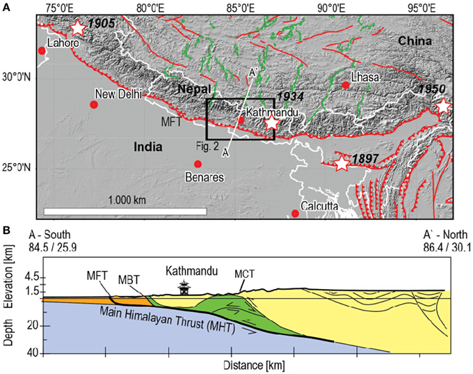
Figure 1. (A) Geodynamic map of Nepal and surrounding, SRTM topography derived shaded relief map, fault lines after the Himalaya Tibet Map (Styron et al., 2010). Open stars: great Himalayan earthquakes since 1895. Solid lines: Main Frontal Thrust (MFT) and other thrusts in red, normal faults in green, country borders in white. The black box shows the area of Figure 2. (B) Cross section with the main tectonic faults, depicting the thin skinned nappe structure of the Kathmandu region after (Avouac et al., 2001). MFT, Main Frontal Thrust; MBT, Main Boundary Thrust; MCT, Main Central Thrust. The Main Himalayan Thrust—MHT connects these faults at depth at a localized detachment plane. This figure is drawn using GMT software.

In April 25, 2015 a magnitude Mw 7.8 earthquake occurred in an area previously identified as a high seismic hazard zone (Giardini et al., 1999). The epicenter with a dominantly thrust type mechanism was located 18-km deep at 84.72°E/28.18°N (GEOFON, 2015). The earthquake was followed by a series of aftershocks, the largest one occurred on 12 May 2015 with Mw 7.3.

These two earthquakes flank the Kathmandu region, Nepal's capital city with more than 1 Million inhabitants, causing over 8500 deaths with an estimated 20–50% of the country's economy being destroyed (CEDIM, 2015). Geologically the Kathmandu region shows a complexity that arises from the presence of doublex type, thin-skinned tectonics, thought to be structurally defined by the Main Frontal Thrust (MFT) to the south and the Main Boundary Thrust (MBT) to the north (Avouac et al., 2001). Sandwiched between these two major faults, different Tertiary sedimentary rocks have been eroded from the basement, and incorporated into a complexly faulted and folded unit (Figure 1B). The area accumulated a 3.5–5.5 km thick sedimentary deposit since the Miocene. It is generally believed that the main décollement of these units locates just atop the Indian basement at ~5–6 km deep beneath the Kathmandu area, as confirmed by different geological and geophysical studies (Avouac et al., 2001). At Kathmandu, the tectonic nappe is locally separated to form a structural Klippe of the Pulchauki Group (Webb et al., 2011).

Here we investigate the 2015 Nepal earthquakes by synthetic aperture radar data that were interferometrically processed to derive the line-of-sight (LOS) displacement of the ground (Bürgmann et al., 2000). Data from different satellites including L-band ALOS-2 and C-band RADARSAT-2 and Sentinel-1 are investigated at different geometries (ascending, descending) to achieve the reconstruction of the coseismic deformation field associated with the Mw 7.8 mainshock on April 25, 2015 and its largest Mw 7.3 aftershock on 12 May 2015, in turn allowing testing different sensors and processing quality for such large earthquake events. Results are analyzed in inverse models to quantify the location and amount of slip at the fault, and to simulate stress interaction between the mainshock and the aftershock, as well as the adjacent faults associated with the tectonic nappes. Important insights can be drawn from this study, such as the potential of other triggered or delayed earthquakes at neighboring or subparallel doublex faults.

Data and Methods

Geodetic Data

For this work we have used SAR products acquired by the ALOS-2, RADARSAT-2, and Sentinel-1 satellites (Supplementary Tables 1, 2). The ALOS-2 data were processed by Lindsey et al. (2015). We processed the Radarsat-2 data using the GAMMA software (Wegmuller and Werner, 1997). The Nepal earthquake was the first large (M > 7.5) earthquake observation application of the Sentinel-1A satellite that was successfully launched on April 3rd, 2014. Its main operational acquisition mode, the Interferometric Wide swath (IW) mode, is operated as a TOPS (Terrain Observation by Progressive Scan) mode (De Zan and Monti Guarnieri, 2006), which provides a large swath with of 250 km at a ground resolution of 5 × 20 m in range and azimuth, respectively (Torres et al., 2012), which is especially well suited for the large 2015 Nepal earthquakes.

Our processing of Sentinel-1 data considers the azimuth-dependent Doppler centroid variation within the burst, both in terms of focusing and interferometric processing (Prats-Iraola et al., 2012). To this aim we compute the offsets between images using a geometric approach, i.e., with the use of an external digital elevation model (SRTM in this particular case) and the precise orbits. With this information the slave image can be accurately interpolated to the slant-range plane of the master image. Afterwards only a global offset needs to be estimated and removed to allow for a continuous phase between bursts. However, in the presence of azimuthal motion, as it happens in the present case, phase jumps occur as a result of the projection of the azimuthal motion into the line of sight, which in the TOPS case is azimuth variant within a burst (De Zan et al., 2014). In order to handle the TOPS geometry accurately, one should consider the true line of sight within a burst, which can be obtained from the geometry and the Doppler centroid under which each point was observed. Selected interferograms are presented in Figures 2, 3 (upper row) along with their simulated displacement and residual (bottom row).

FIGURE 2

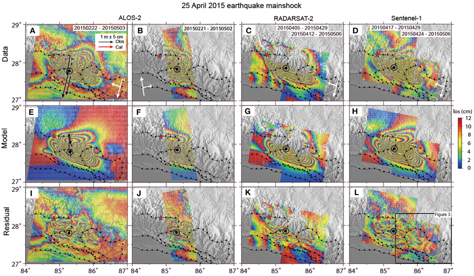
Figure 2. Earthquake mainshock, as seen from radar satellites that allow quantifying displacements in the Line of Sight (LOS) as indicated by white arrow in (A–D). Upper row is the data (A, B, wideswath ALOS-2; C, RADARSAT-2 from two tracks, and D, Sentinel-1 from two tracks). Center row (E–H) is the model solution. Bottom row (I–L) shows the residual after subtracting the model from the data. Red star depict the location of the mainshock epicenter, located to the west of the deformation area. Fault lines are the MFT, MBT, and MCT from south to north, after (Webb et al., 2011). Kathmandu shown by black circle. The black insert box shown on (I) is shown the area of the largest aftershock shown in Figure 3. This figure is drawn using GMT software.

FIGURE 3

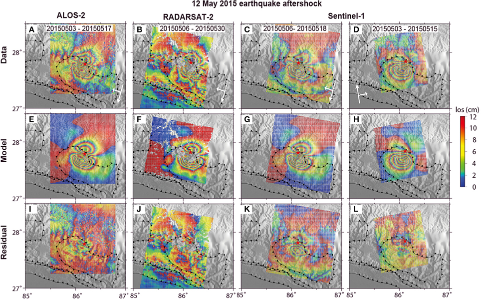
Figure 3. Largest recorded earthquake aftershock, as seen from radar satellites, LOS as indicated by white arrow in (A–D). Upper row is the data (A, wideswath ALOS-2; B, RADARSAT-2; and C,D, Sentinel-1 from ascending and descending views). Center row (E–H) is the model solution. Bottom row (I–L) shows the residual after subtracting the model from the data. Red star depicts the location of the aftershock epicenter, located to the west of the main deformation area. Fault lines are the MFT, MBT, and MCT from south to north, after (Webb et al., 2011). Kathmandu is shown by black circle. This figure is drawn using GMT software.

The InSAR data were all processed using a 30 m (RADARSAT-2) or a 90 m (ALOS-2 and Sentinel-1) SRTM digital elevation model. The RADARSAT-2 required high resolution DEM because its data (this particular extra-fine beam) is of much higher resolution than ALOS-2 and Sentinel-1 data. The orbital effect was removed from the ALOS-2 data by estimating a linear gradient far from the earthquake deformation (Lindsey et al., 2015). For RADARSAT-2 and Sentinel-1 data, this effect was considered during the inversion process (see Section Data Handling and Modeling Method).

Global Positional System (GPS) data are available from a network that has been installed and operated by Caltech Tectonics Observatory. For the 2015 Nepal earthquake, raw data was provided by Jean-Philippe Avouac (Caltech), which was processed with the GIPSY-OASIS software and JPL Final orbits and clock products by Advanced Rapid Imaging and Analysis (ARIA) at JPL (Galetzka et al., 2015). In this study GPS data were used for InSAR data validation and also for model simulation (Figure 2, black vectors).

Data Handling and Modeling Method

To improve the computation efficiency, the original InSAR data were uniformly down-sampled to 2 arcmin and 1 arcmin for the mainshock data and the strongest aftershock, respectively. The MHT is sub-horizontal in this area and our data coverage is essentially uniform leading to a uniform distribution of resolution and sensitivity on our fault geometry. This allows us to apply a uniform downsampling to the InSAR data (Lohman and Simons, 2005).

A constrained least squares method presented in Wang et al. (2013) was used to invert for the slip models, in which an a-priori smoothing constraint was added to make the solution stable and equitable. Similar least squares method has been widely used for slip model inversion elsewhere (e.g., Freymueller et al., 1994; Reilinger et al., 2000). The steepest descent method was applied to search for the optimal solution, by considering the cost function defined as:

$\begin{array}{cc}\text{F}\left(s\right)=||\text{G}s-y|{|}^2+{\alpha }^2||\text{H}s|{|}^2& (1)\end{array}$

where s is the slip vector of each sub-fault on the fault plane; G is the Green's function matrix calculated based on a layered crustal structure (Crust 2.0); y is the data consisting of InSAR LOS and GPS displacements; H represents the finite difference approximation of the Laplacian operator; α is the smoothing factor, which controls the trade-off between model roughness and misfit. Fault planes with spatial scales of 250 × 120 km² and 100 × 120 km² were set up for the mainshock and the largest aftershock, which were then subdivided into patches with the constant size of 10 × 10 km². We used a simple method dealing with data errors, where the correlation of the InSAR data was neglected. We estimated the mean RMS error of InSAR observation using the far-field data misfits derived from initial model inversions (5 cm). We also considered the error of InSAR data collected by different satellites. However, they are similar and all close to 5 cm (5.45, 4.61, and 5.24 cm for ALOS-2, Sentinel-1, and Radarsat-2 data). We thus use a uniform error of 5 cm for all InSAR data.

We initially carried 3D search of the fault location and dip angle based on ALOS-2 data and GPS data. However, the horizontal location of the fault could not be resolved due to the nearly planar geometric feature (Supplementary Figure 1). We thus fixed the up edge of the fault plane based on geological map (Figure 1A), and searched for the dip angle using the data misfits (Supplementary Figure 2). The optimal smoothing factor was selected based on the trade-off curve drawing the data misfit as a function of the model roughness (smoothing factor, Supplementary Figure 2). The same smoothing factor (0.15) was used for all inversions in order to compare the models derived from different dataset. We constrained the rake angles of each sub-fault to vary between 45° and 135° based on focal mechanism and tectonic background. We estimated the possible total offsets existing in the unwrapped deformation fields and removed them from the observation. The orbital effect of the RADARSAT-2 data and Sentinel-1 data were estimated by fitting a ramp based on the far-field model residuals. We didn't estimate the orbital effect directly from far-field observation as the far-field data could also be affected by earthquake deformation for RADARSAT-2 and Sentinel-1 frames (Figure 2).

We carried out joint inversions of InSAR data acquired by different satellites and GPS data; Then, a joint inversion of all InSAR data and GPS data was performed and the derived model was regarded as the final model. In the joint inversion, the Helmert variance component estimation (HVCE) method (Xu et al., 2010) was applied to determine the relative weighting between InSAR and GPS data. The final weighting between InSAR and GPS convergences to 1:3.6, close to the value derived by Wang and Fialko (2015). We also try different weighting factors and no clear change of the inverted result was observed (Supplementary Figure 3). Two methods were used to estimate the spatial resolving power of all InSAR data and GPS data: one is the so-called checkerboard test; the other one is to derive the sensitivity operator of each fault patch (Sum of the partial derivatives relating InSAR and GPS displacements to unite slip; Loveless and Meade, 2011).

Results

Deformation at the Kathmandu Window

The largest spatial coverage is available from the L-band ALOS-2 observations, allowing a full and highly coherent view onto the deformation area from both ascending and descending perspectives. The coseismic deformation field (Figure 2) consists of two main zones, an uplift zone around Kathmandu basin and a wider subsidence to its north with a hinge-line in-between at Lon/Lat 27.85/85.75° and 27.93/85.04°. The uplift zone marked by ALOS-2 data is elliptic and stretches WNW-ESE covering a region ~7000 km² around Kathmandu (Figure 2, top row). The maximum vertical displacement is found 20 km to the NE of Kathmandu city at Lon/Lat 27.74/85.50°. To the north, a larger area of ~9000 km², though at a smaller scale, shows LOS subsidence. The position of the hinge-line, and the stronger amplitude but smaller spatial extend of uplift in the south of this line, already suggests a north-dipping thrust fault plane located to the north of Kathmandu. In contrary, the RADARSAT-2 and Sentinel-1 data, both working in C-band, only delineate part of the coseismic deformation field well. Due to large displacement gradient, the correct number of fringes in the peak displacement region might be slightly underestimated for the C-band sensors, but overall the different data show the similar pattern and amount of ground deformation. The GPS data can be explained almost equally well by slip models that were derived from different datasets. Details of these data are investigated in the modeling section detailed below.

The Source of the Deformation Signals

Model computations were performed for different InSAR data separately, and the results were compared. Combined with GPS, these data can give similar pattern and rupture location of both the mainshock (Figure 2) and the largest aftershock (Figure 3).

With a maximum slip of ~5.2 m, the spatial scale of the main rupture is 150 and 50 km along strike and dip, respectively. The main rupture of the largest aftershock being 40 × 20 km along strike and dip directions locates just at the eastern margin of the main coseismic slip.

Thrust slip is dominant for both the mainshock and the largest aftershock, but we also observe a consistent right lateral strike slip motion (Figure 4). While for all InSAR data and the L-band InSAR data the area of peak slip appears more extended, the C-band data shows a slightly less pronounced peak slip area. By comparing the geodetic moment magnitude, we find that all slip inversions suggest a very consistent moment release of Mw 7.80–7.81 for the mainshock, and Mw 7.25–7.40 for the largest aftershock, consistent with the seismic estimates of Mw 7.8 and Mw 7.3, respectively (Figure 4).

FIGURE 4

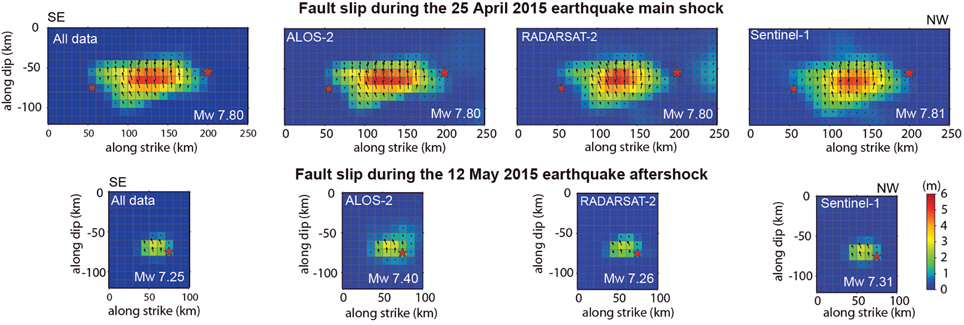
Figure 4. Fault models showing the distribution (colors) and the direction (vectors) of the slip at the main earthquake fault and at the aftershock fault for different data. Fault models were calculated for the different satellites. For each satellite more than one track or viewing geometry was available.

Considering different weights for the GPS data can slightly change the slip maximum, but the rupture scale and pattern remains stable (Supplementary Figure 3). Although the earthquakes are well captured by all three satellites, the C-band InSAR data appears to have a poorer precision on the northern margin of the slip distribution, which might be related to the steep topography and mountainous region in this area, the associated lower coherence, and/or the lack of a good coseismic ascending geometry available by these satellites. Due to the high degree of similarity of the slip models, the joint inversion of all data does not significantly affect the model (Figure 4). Both the checkerboard test and the calculated sensitivity operator reveal that the slip on fault patches can be well resolved based on the available geodetic data (Supplementary Figure 4).

The residual plots show that the inverted slip models can explain the observed LOS displacements well, although some residual deformation are still observed near the main rupture area, which perhaps mainly relate to some local deformation or a more complex geometry of the rupture plane (Figure 2). Overlaying the cross section of the slip plane to the geodynamic cross section (Avouac et al., 2001) we find that the optimized slip plane almost exactly coincides with the Main Himalaya Thrust (MHT) that is well constrained beneath the Kathmandu basin (Figure 5). As the MHT is associated to a thin skinned double structure and assorted sub-parallel faults, it becomes of interest if the mainshock may have encouraged slip at one or several of the neighboring faults.

FIGURE 5

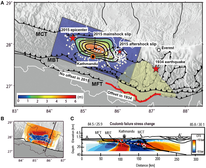
Figure 5. (A) Synthesis map. Red stars: great Himalayan earthquakes, in 1934 the Mw 8.2 Bihar earthquake, and in 2015 the Gorkha earthquake, white dots: earthquake aftershocks. The main fault displacement locates just to the north of Kathmandu (shown by red circle), where amount of slip is color coded and peaks at ~5.2 m (color and black contours with interval of 1 m). The largest aftershock is located just to the east of the slip area and peaks at 2.5 m (white contours with interval of 1 m). InSAR data from three different satellites could not reveal any coseismic rupture associated with any of the main thrusts (MFT, MBT, MCT). This contrasts to the interpretation of the 1934 earthquake, where significant displacement at the MFT was inferred (Sapkota et al., 2013). (B) Coulomb failure stress (CFS) on the main rupture plane. The CFS has decreased at the slip area, and increased in the surrounding. (C) Cross section with the main fault lines (Avouac et al., 2001) and CFS calculated by the coseismic mainshock slip model, where red denotes a stress built up, and blue a stress shadow. The updip and downdip areas receive large CFS built up. Note that the downdip area has experienced the largest aftershock (white star), whilst the updip region so far did not display any rupture. This figure is drawn using GMT software.

Stress Transfer

Using the optimal slip model as constrained from L-band InSAR and GPS data, we calculated the Coulomb Failure Stress (CFS) change on the fault plane and surrounding medium (Figure 5). Computing the CFS change following an earthquake tells whether a fault has been brought closer or away from rupture (Stein, 1999) and has been applied specifically to the Himalayas (Bollinger et al., 2004). Our models are loaded by the earthquake mainshock, and the receiving plane is subparallel to this mainshock plane. The CFS has significantly decreased in the main rupture area of the mainshock, as expected. In contrast, the CFS was highly increased in area surrounding the main rupture, especially at the down-dip and up-dip area of the main rupture (Figure 5). One of the largest stress build up regions is found at the eastern area down-dip of the main rupture, which coincides with the location of the largest aftershock.

A frictional ration of 0.7 and a dip angle of 10° were used in these results, but we also explored different frictional ratio (0.5–0.9) and dip angle of receiver fault (5°–20°). No significant difference was observed for the obtained CFS, implying that the models are robust and support the hypothesis that earthquakes can be triggered at the downdip end of the mainshock. Similarly, also earthquakes may be encouraged at the updip end and laterally of the mainshock. The subparallel faults, in turn, experience a negative CFS.

Discussion

The 2015 Gorkha earthquake was a rare event, causing significant shortening without primary surface ruptures. The event uplifted of the Lesser Himalaya at south, but lowered the Greater Himalaya at north. Abundant landslides have been triggered, causing unstable rock slopes to fail and snow avalanches at Mount Everest, some 140 km away from the earthquake rupture center. The number of aftershocks is slowly decaying, although still others and large earthquakes may follow. In this work we utilized different InSAR data to create a detailed image of the earthquake mainshock and its largest aftershock. We find that slip is slightly oblique, i.e., with a dextral component, and exceeds a peak thrust slip of about 5.2 m. The slight oblique nature of the MHT is in line with long term GPS observations, also revealing a dextral motion component (Kundu et al., 2014). The Kathmandu city is overlaying the region of the highest slip to the south (Figure 5), but no primary fault ruptures have been observed in town, or at any of the main thrusts (MFT, MBT, MCT), neither by eyewitness accounts nor in our InSAR data. Therefore, the further seismotectonic development is of major interest for scientists and population there alike, as a delayed effect may still be expected at the shallow part of the fault.

Limitations

The herein described dataset is an exceptionally unique InSAR dataset for the study of earthquake, with different views (ascending and descending) from different satellites (ALOS-2, RADARSAT-2, Sentinel-1). Although the data appear very consistent, so that by adding or deleting a specific satellite view the fault slip model is not substantially affected, our study and the interpretations could have been affected by various sources of error in data, processing or modeling. For example, the spatial extent of the retrieved deformation area differs between C-band and L-band, and results from a different coherence. In this regard the L-band system performed best in the mountainous and vegetated area north of Kathmandu. The amount of LOS displacements and the displacements appear to be very similar, although being difficult to access quantitatively because of dissimilar viewing geometries of the satellites. The inverted slip distribution models, in turn, show a very consistent pattern at the fault patches, with similar amplitude. To even further evaluate the accuracy of our results, we cross-checked them with GPS data that were made available by Caltech, showing an excellent fit. Because we did not employ an InSAR time series, time dependent filtering approaches that could minimize atmospheric artifacts were not implemented.

Implications

The processes associated with great Himalayan earthquakes have been puzzling for centuries, as albeit significant damage has occurred historically, some large (M8+) earthquakes have reached the MFT and break the surface (Sapkota et al., 2013), while other smaller (M7+) events left no trace of surface rupture, remaining blind, including the 1905 Kangra earthquake and the 1833 events. From the geodetic data and slip modeling results presented in this paper, we conjecture that the 2015 Gorkha earthquake, which happened just beneath the capital city, did not show any sign of major ruptures at the surface.

Coulomb stress calculations reveal that the faults being adjacent to the seismogenic fault experienced a significant stress increase. In fact, those faults that have been inferred as active are the ones that have been brought even closer to failure now. The sub-parallel faults of the thin skinned nappes, in turn, experience a decrease of Coulomb failure stress, meaning that slip at sub-parallel thin skinned nappe tectonics is currently not favored. The decrease of the CFS may explain why at the sites above the main rupture no primary faulting has been observed. The interplay between the shallowly inclined faults that localize the strain in the thickening crust must therefore be considered in the seismic cycle, where the coseismic stage discourages slip at the nappe faults. Contrarily, interseismic deformation may well take place at these subparallel fault structures. Moreover, one might hypothesize that these structures are not active at all, which warrants to be further elaborated in future studies.

An interesting phenomenon is seen in the apparent lack of slip in the Himalayan front to the up-dip area of the fault. Our CFS computations suggest a major stress build up at the MFT, MBT and also at the lower portion of the MCT. The same fault traces, however, evidently lack a coseismic displacement detectable by our InSAR data (Figure 2). As the CFS models suggest a stress build up at the MFT and the MCT, one may speculate whether these might be regions of an anticipated slip event, possibly associated with postseismic effects that may act for years (Monsalve et al., 2009). Historical earthquakes have shown that the MFT caused a displacement over considerable length, which was 150 km long after the 1934 Bihar-Nepal earthquake (Sapkota et al., 2013). As the 1934 Bihal-Nepal earthquake occurred just to the east of the 2015 Gorkha earthquake, we conjecture that the geological setting and seismogenic mechanism might be comparable. Therefore, close observation of the MFT, MBT, and MCT in the coming months to years might be warranted to test whether slip at the thrusts is occurring as a delayed consequence of the stress redistribution as shown in this paper. Similarly, the region to the west of the 2015 earthquake has been experiencing a stress built up (Figure 5). Given that the previous earthquake and the 2015 earthquake display an east-to-west directivity, the region west of the Gorkha earthquake is considered by us as an area that needs to be closely monitored in future.

Conclusions

We used multi-satellites InSAR data and GPS data to create a detailed slip image of the mainshock and its large aftershock of the Mw 7.8 Gorkha earthquake. Our results suggest that this event occurred on a planar fault geometry with a shallow dip angle of 10°, which is consistent with the thin skinned MHT. The main shock ruptured the MHT with a scale of 150 × 50 km in strike and dip direction at the deep portion of the seismogenic fault. The strong aftershock occurred at the southeast tip of the main rupture with a scale of 40 × 20 km. With slip maximum of 5.2 and 2.7 m, the inferred geodetic moment magnitude of the mainshock and the strong aftershock is 7.8 and 7.3 respectively. No slip was observed at the shallow part (depth < 5 km), which shows clear contrast with the 1934 Bihar-Nepal earthquake. Combined with the CFS change our results imply increased seismic hazard at the shallow part and the west part of the rupture fault.

Author Contributions

FD and TW contributed to data analysis, modeling, and manuscript writing; RW contributed to result analysis and modeling. MM, PP, and SS processed the C-band InSAR data; all authors reviewed the manuscript.

Conflict of Interest Statement

The authors declare that the research was conducted in the absence of any commercial or financial relationships that could be construed as a potential conflict of interest.

Acknowledgments

We appreciate discussions with the INSARAP team and the GFZ Hazard Team on an earlier version of this paper. We exploited Copernicus data (2015), the processing and analysis was made as a contribution to the ESA SEOM INSARAP project (ESA-ESRIN Contract 4000110587/14/I-BG), and the HGF Helmholtz Alliance on Remote Sensing and Earth System Dynamics (EDA). ALOS-II original data are the copyright of Japan Aerospace Exploration Agency (JAXA) and were provided through the research proposal (No. 1161). We thank the Canadian Space Agency for providing RADARSAT-2 data. This work was partly supported by NSFC (No. 41304017). Some of the figures were made using the GMT software (Wessel and Smith, 1991). The data of this paper are available from the corresponding author.

Supplementary Material

The Supplementary Material for this article can be found online at: https://www.frontiersin.org/article/10.3389/feart.2015.00065

References

Ader, T., Avouac, J. P., Liu-Zeng, J., Lyon-Caen, H., Bollinger, L., Galetzka, J., et al. (2012). Convergence rate across the Nepal Himalaya and interseismic coupling on the Main Himalayan Thrust: implications for seismic hazard. J. Geophys. Res. 117, B04403. doi: 10.1029/2011jb009071

CrossRef Full Text | Google Scholar

Avouac, J. P., Bollinger, L., Lave, J., Cattin, R., and Flouzat, M. (2001). Seismic cycle in the Himalayas. C. R. Acad. Sci. II A. 333, 513–529.

Bollinger, L., Avouac, J. P., Cattin, R., and Pandey, M. R. (2004). Stress buildup in the Himalaya, J. Geophys. Res. 109, B11405. doi: 10.1029/2003JB002911

CrossRef Full Text | Google Scholar

Bürgmann, R., Rosen, P. A., and Fielding, E. J. (2000). Synthetic aperture radar interferometry to measure Earth's surface topography and its deformation. Annu. Rev. Earth Pl. Sci. 28, 169–209. doi: 10.1146/annurev.earth.28.1.169

CrossRef Full Text | Google Scholar

CEDIM (2015). Nepal Earthquakes – Report #3, ed KIT-GFZ. Potsdam: CEDIMForensic Disaster Analysis Group, CATDAT and Earthquake-Report.com.

De Zan, F., and Monti Guarnieri, A. (2006). TOPSAR: terrain observation by progressive scans. IEEE Trans. Geosci. Remote Sens. 44, 2352–2360. doi: 10.1109/TGRS.2006.873853

CrossRef Full Text | Google Scholar

De Zan, F., Prats-Iraola, P., Scheiber, R., and Rucci, A. (2014). “Interferometry with TOPS: coregistration and azimuth shifts,” in Paper Presented at EUSAR 2014 10th European Conference on Synthetic Aperture Radar, Proceedings of VDE (Berlin).

Google Scholar

Freymueller, J., King, N. E., and Segall, P. (1994). The coseismic slip distribution of the Landers earthquake. Bull. Seismol. Soc. Am. 84, 646–659.

Google Scholar

Galetzka, J., Melgar, D., Genrich, J. F., Geng, J., Owen, S., E. O., Lindsey, et al. (2015). Slip pulse and reso-nance of Kathmandu basin during the 2015 mW 7.8 Gorkha earthquake, Nepal imaged with geodesy. Science 349, 1091–1095. doi: 10.1126/science.aac6383

PubMed Abstract | CrossRef Full Text

GEOFON (2015). Report for the Nepal Earthquake, ed GFZ. Potsdam: Deutsches GeoForschungsZentrum.

Giardini, D., Grunthal, G., Shedlock, K. M., and Zhang, P. Z. (1999). The GSHAP Global Seismic Hazard Map. Ann. Geofis 42, 1225–1230.

Google Scholar

Kundu, B., Yadav, R. K., Bali, B. S., Chowdhury, S., and Gahalaut, V. K. (2014). Oblique convergence and slip partitioning in the NW Himalaya: implications from GPS measurements. Tectonics 33, 2013–2024. doi: 10.1002/2014TC003633

CrossRef Full Text | Google Scholar

Lavé, J., Yule, D., Sapkota, S., Basant, K., Madden, C., Attal, M., et al. (2005). Evidence for a great medieval earthquake (approximate to 1100 AD) in the Central Himalayas, Nepal. Science 307, 1302–1305. doi: 10.1126/science.1104804

PubMed Abstract | CrossRef Full Text | Google Scholar

Lindsey, E., Natsuaki, R., Xu, X., Shimada, M., Hashimoto, H., and Sandwell, D. (2015). Line of sight deformation from ALOS-2 interferometry: Mw 7.8 Gorkha earthquake and Mw 7.2 aftershock. Geophys. Res. Lett. 42, 6655–6661. doi: 10.1002/2015GL065385

CrossRef Full Text | Google Scholar

Lohman, R. B., and Simons, M. (2005). Some thoughts on the use of InSAR data to constrain models of surface deformation: noise structure and data downsampling. Geochem. Geophy. Geosyst. 6, Q01007. doi: 10.1029/2004GC000841

CrossRef Full Text | Google Scholar

Loveless, J. P., and Meade, B. J. (2011). Spatial correlation of interseismic coupling and coseismic rupture extent of the 2011 mW = 9.0 Tohoku-Oki earthquake. Geophys. Res. Lett. 38, L17306. doi: 10.1029/2011GL048561

CrossRef Full Text | Google Scholar

Monsalve, G., McGovern, P., and Sheehan, A. (2009). Mantle fault zones beneath the Himalayan collision: flexure of the continental lithosphere. Tectonophysics 477, 66–76. doi: 10.1016/j.tecto.2008.12.014

CrossRef Full Text | Google Scholar

Mugnier, J. L., Gajurel, A., Huyghe, P., Jayangondaperumal, R., Jouanne, F., and Upreti, B. (2013). Structural interpretation of the great earthquakes of the last millennium in the central Himalaya. Earth-Sci. Rev. 127, 30–47. doi: 10.1016/j.earscirev.2013.09.003

CrossRef Full Text | Google Scholar

Prats-Iraola, P., Scheiber, R., Marotti, L., Wollstadt, S., and, Reigber, A. (2012). TOPS interferometry with TerraSAR-X. IEEE Trans. Geosci. Remote Sens. 50, 3179–3188. doi: 10.1109/TGRS.2011.2178247

CrossRef Full Text | Google Scholar

Reilinger, R. E., Ergintav, S., Bürgmann, R., McClusky, S., Lend, O., Barka, A., et al. (2000). Coseismic and postseismic fault slip for the 17 August, M = 7.5, Izmit, Turkey earthquake. Science 289, 1519–1524. doi: 10.1126/science.289.5484.1519

PubMed Abstract | CrossRef Full Text | Google Scholar

Sapkota, S. N., Bollinger, L., Klinger, Y., Tapponnier, P., Gaudemer, Y., and Tiwari, D. (2013). Primary surface ruptures of the great Himalayan earthquakes in 1934 and 1255. Nat. Geosci. 6, 71–76. doi: 10.1038/ngeo1720

CrossRef Full Text | Google Scholar

Stein, R. S. (1999). The role of stress transfer in earthquake occurrence. Nature 402, 605–609. doi: 10.1038/45144

CrossRef Full Text | Google Scholar

Styron, R., Taylor, M., and Okoronkwo, K. (2010). HimaTibetMap-1.0: new ‘web-2.0’ online database of active structures from the Indo-Asian collision. Eos 91, 181–182. doi: 10.1029/2010EO200001

CrossRef Full Text | Google Scholar

Torres, R., Snoeij, P., Geudtner, D., Bibby, D., Davidson, M., Attema, E., et al. (2012). GMES Sentinel-1 mission, GMES Sentinel-1 mission. Remote Sens. Environ. 120, 9–24. doi: 10.1016/j.rse.2011.05.028

CrossRef Full Text | Google Scholar

Wang, K., and Fialko, Y. (2015). Slip model of the 2015 mW 7.8 Gorkha (Nepal) earthquake from inversions of ALOS-2 and GPS data. Geophys. Res. Lett. 42, 7452–7458. doi: 10.1002/2015GL065201

CrossRef Full Text | Google Scholar

Wang, R. J., Parolai, S., Ge, M. R., Jin, M. P., Walter, T. R., and Zschau, J. (2013). The 2011 M-w 9.0 Tohoku Earthquake: comparison of GPS and Strong-Motion Data. Bull. Seismol. Soc. Am. 103, 1336–1347. doi: 10.1785/0120110264

CrossRef Full Text | Google Scholar

Webb, A. A. G., Schmitt, A. K., He, D. A., and Weigand, E. L. (2011). Structural and geochronological evidence for the leading edge of the Greater Himalayan Crystalline complex in the central Nepal Himalaya. Earth Planet Sci. Lett. 304, 483–495. doi: 10.1016/j.epsl.2011.02.024

CrossRef Full Text | Google Scholar

Wegmuller, U., and Werner, C. (1997). “Gamma SAR processor and interferometry software,” in The 3rd ERS Symposium on Space at the Service of our Environment, (Florence).

Google Scholar

Wessel, P., and Smith, W. H. F. (1991). Free software helps map and display data. EOS Trans. Am. Geophys. Union. 72, 445–446.

Google Scholar

Xu, C., Liu, Y., Wen, Y. M., and Wang, R. (2010). Coseismic slip distribution of the 2008 mW 7.9 Wenchuan earthquake from joint inversion of GPS and InSAR Data. Bull. Seis. Soc. Am. 100, 2736–2749. doi: 10.1785/0120090253

CrossRef Full Text | Google Scholar