Improving Low-Relief Coastal LiDAR DEMs with Hydro-Conditioning of Fine-Scale and Artificial Drainages

Introduction

Technological advances in Light Detection and Ranging (LiDAR) have spurred extensive new applications in coastal hazards management and research on coastal processes. Coastal LiDAR has also pioneered digital terrain modeling in low-relief landscapes stemming from early work on NASA Airborne Topographic Mapping (ATM) LIDAR on the Greenland Ice Sheet (Krabill et al., 2000). The ATM LiDAR led to a series of extensive beach mapping efforts by NOAA Coastal Services Center (now, the NOAA Office for Coastal Management). Beach mapping LiDAR further expanded to the USA west coast, Hawaii and territories, even as data acquisition hardware, airborne platforms, and processing techniques improved. As a result, the literature on coastal LiDAR is among the richest in modern digital terrain modeling applications and diverse user groups engaged, ranging from coastal geomorphology, storm surge and inundation modeling, and coastal resource and habitat assessment. In addition, as data collections expanded temporally, change analysis techniques have developed and been refined, data extraction techniques arisen, and a more mature understanding of elevation data quality and error have been achieved. This paper addresses these improvements and the impetus for expanding LiDAR to even greater coverage globally for its significant contributions to sustainable human development and environmental management on coasts. Given the long history of coastal LiDAR in North Carolina (NC), USA, and its relatively rich data repository, a focus on methods and a case study from NC is provided. A major advantage of LiDAR over other terrain mapping technologies is its accuracy in low elevation, even micro-relief topographic settings. Yet extensive, flat coastal plains still present challenges, such as agricultural ditches, salt marshes, swamp forests with variable understory vegetation, and inherent micro-scale topographic and hydrologic gradients. Our goal in this paper is to succinctly review developments of LiDAR-derived bare earth (BE) Digital Elevation Models (DEMs) pertaining to flood-prone, low-relief coastal plains. This review will aim to succinctly capture methods and improvements achievable by DEM inspection, hydro-conditioning, and definitive corrections. Secondly, we present a methodology for improving the characterization of artificial ditches in BE DEMs and demonstrate and evaluate this technique in a case study of the ultra-low-relief area of Moyock in northeastern North Carolina.

Coastal LiDAR Applications

Application to Coastal Resource Inventory

Coastal LIDAR has developed enhanced capabilities for resource inventory and monitoring. LIDAR has successfully differentiated coastal vegetation, such as invasive Phragmites australis from other salt and brackish marshes (Yang and Artigas, 2010; Allen, 2014), mapped submerged aquatic vegetation (SAV) (Brock et al., 2004; Brock and Purkis, 2009), and assessed changes in landforms and habitat along beach-dune systems (Mitasova et al., 2005; Stockdon et al., 2009). In low-relief areas such as coastal North Carolina, vast areas of wetland and agricultural are vulnerable to coastal flooding from sea-level rise. Studies such as Poulter and Halpin (2008) have demonstrated the need for representing the hydrologic linkages in these landscapes and the limited value of coarse-scale DEMs or even LiDAR without the adequate resolution to characterize topographic complexities and model hydrologic connectivity. In addition, studies have explored the need for LiDAR corrections of vegetated salt marsh surfaces, such as empirical correction techniques (Hladik and Alber, 2012). To improve accuracy and potential modeling applications, coastal LiDAR must make further strides to reduce vertical DEM errors, but also to better characterize hydrologic paths for runoff, tidal, and storm inundation processes.

Emphasis on Beaches and Barrier Islands

Beaches and barrier islands have attracted great interest in coastal LiDAR applications. Many of these applications stem from NASA ATM LiDAR on the Greenland Ice Sheet and experimentally applied to Assateague Island National Seashore (Krabill et al., 2000). LiDAR beach mapping efforts were subsequently expanded by to USA west coast, Hawaii and territories, even as data acquisition hardware, airborne platforms, and processing techniques improved with its commercialization. The literature on coastal LiDAR is among the richest in contemporary digital terrain modeling and has broad user groups engaged, ranging from coastal geomorphology, storm surge and inundation modeling, to coastal resource, development, and habitat assessment. In addition, as data collections expanded temporally, change analysis techniques have developed and been refined, data extraction techniques arisen, and a more mature understanding of elevation data quality and error has been achieved. This paper addresses these improvements and the impetus for expanding LiDAR to even greater coverage globally for its significant contributions to human development and environmental management of low-lying coasts.

While coastal LiDAR data extent and availability have increased, some have noted the crucial technical aspect of data acquisition regarding ground post-pacing density and subsequent DEM accuracy (e.g., Raber et al., 2007). This important factor has also been evaluated in hydrologic characterization and correction techniques in coastal LiDAR DEMs, such as ditches and streams (Poppenga et al., 2013). A major advantage of LiDAR over other terrain mapping technologies is its accuracy in low elevation, even micro-relief topographic contexts, and North Carolina's coastal plain comprises a relevant assemblage of a trailing-edge continental margin with wide, low-relief coastal plains, submergent estuaries, drowned deltas, upland peaty “pocosin” vegetation, and barrier islands. Hence, a North Carolina case study offers a microcosm of potential applications and lessons that can be applied extensively elsewhere.

Hurricane Floyd in North Carolina

Beyond resource inventory and management, LiDAR has a widely recognized capability for flood inundation and physical asset mapping, with numerous examples globally (Webster et al., 2004). A critical event occurred in North Carolina on September 16, 1999, when Hurricane Floyd struck the coast, succeeding two prior tropical cyclones. Floyd was a minimal category 1 storm by wind standards, but nonetheless dropped extensive rainfall on already highly saturated soils immediately after Hurricane Dennis earlier in August. Although Floyd was not extraordinarily remarkable or singular for its wind, or even heavy precipitation, it nonetheless induced a major flood event, circa 150–200 years recurrence interval flooding (Barnes, 2001). The major Tar-Pamlico, Neuse, Cape Fear, and Roanoke River basins received enormous rainfall amounts on already high flood stage conditions, resulting in a record 8.3 m flood at Greenville, NC. These floods resulted in North Carolina's largest natural disaster, including US$7.8B damage and 52 lives lost in North Carolina, mostly related to flood aftermath (Barnes, 2001). The flood extent from Floyd generated incredible public interest in flood mapping, flood insurance, and emergency management, as prior flood maps corresponding to the expected rainfall and prior flood risk estimates were dramatically erroneous underestimates in many situations. These pre-Lidar (FEMA Q3) flood maps showed deficiencies and created impetus for a massive LiDAR elevation mapping campaign. In addition, thousands of farm animals and agricultural operations, transportation, and public utilities were affected by Hurricane Floyd floods, many of which were not digitally mapped at that time for emergency managers to respond. Following the disaster, the State of North Carolina and the US Federal Emergency Management Agency (FEMA) instituted a technology partnership (NCFMP, 2002), to develop and showcase new technologies for flood mapping and disaster management (NCFMP, 2015). In the ensuing years, North Carolina would develop statewide LiDAR elevation data, re-map its floodplains, and showcase new state-of-the-art processes for floodplain mapping and management as guidance to post-disaster recovery and planning. Fortuitously, these rich datasets would also yield several indirect benefits, including LiDAR applications research in geomorphology and derivative coastal hazards, such as hydrodynamic modeling of storm surges, geophysical and geologic research, and investigation of coastal processes, sea level rise, and change dynamics on barrier islands.

Hydrologic Characterization in DEMs

Among the major advances in floodplain mapping using LiDAR has been the advancement of more accurate hydrologic representation and derived modeling. Maune et al. (2007) detail the need and accepted procedures to improve DEM terrain representation around hydrologic features, specifically the process of “Hydrologic enforcement” (or “Hydro-enforcement”) which can include digitized breakline features being added to the spatial interpolation process. Now accepted by the FEMA for production of floodplain delineations, 2D and 3D breaklines are a routine component of the workflow for LiDAR analysis and production of DEMs and DTMs. Coastal plains such as North Carolina's may have landform features more subtle than the standard rivers, streams and lake, or estuary waterbodies, which are generally easier to delineate 2D or 3D breakline features. Bridges, as an example, are more widely recognized as a feature that will require manual correction “cut” into breaklines. Maune et al. (2007) further recommend that ditch and stream centerlines normally be used as drainage breaklines and hydro-enforced in TINs.

DEM Inspection

In advance of applying hydro-correction, it is worth noting the utility of data assessment for any given study area or LiDAR dataset to determine the need and extent of hydro-correction. Hutchinson and Gallant (2000) promote the use of drainage analysis and full catchment delineation of watershed boundaries and stream networks, visual inspection of shaded relief, and contour mapping, as steps to aid identification of potential sinks in DEMs. Gallant and Wilson (2000) caution against global application of processes that might assumedly “burn in” stream lines into DEMs, as these may cause the slope of surrounding DEM pixels to change, resulting in multiple flowpaths for wide or multi-cell width stream networks. In addition to better understanding the representation of a given study area in DEMs, a concerted phase of review for data quality and landform representation in DEMs could also inform subsequent selection of enforcement or conditioning techniques. DEM inspection in the context of low-relief topography and areas replete with artificial canals or ditches warrants additional consideration of the potential for flow runoff or inundation conduits in these linear features.

Hydro-enforcement and Conditioning

Whereas, hydro-correction focuses upon 3D terrain objects and representation in a resulting DEM, the process of “Hydrologic conditioning” attempts to rectify artifacts in DEMs to improve the simulation of continuous water flow across the overall terrain. A significant artifact of the interpolation of LiDAR mass points, even with 2D and 3D breaklines and hydrologic enforcement, artificial pits or sinks are common. Conditioning seeks to fill these sinks and/or better represent their linkages and connectedness as actual features and conduits of flow. Fine-scale features such as culverts, catch-basins, and agricultural ditches thus often present the need for careful assessment of sinks to determine if they are real features and, especially, to condition them to drain properly in a DEM. It is highly desirable that such features as ditches, culverts, and related potential sink points be captured and integrated in the process of hydrologic conditioning, preferably from a local community GIS database (Maune, 2007). In circumstances where ditches are not mapped a priori for a LiDAR campaign and incorporated into the processing and interpolation, conditioning steps can play an important role. In such cases, a given DEM can be re-conditioned, or corrected, post-hoc, by mapping and vector-raster spatial analysis. The case study below illustrates a new methodology for post-processing and hydrologically conditioning DEMs in low-relief coastal plains where extensive agricultural or other drainage ditches strongly influence hydrology.

Materials and Methods

Study Area: Moyock, North Carolina, USA

This technique was used near the Town of Moyock, in Currituck County, North Carolina, USA, (Figure 2) to enhance the hydrologic representation of small ditches in a 6 m resolution LiDAR DEM. The Moyock area is situated on the outer coastal plain of North Carolina, with extensive low-lying pocosin natural vegetation in poorly-drained upland terraces and extensive freshwater non-tidal marshes and swamp forests draining south into the Albemarle Sound. The area was extensively ditched and canalled to drain the uplands for agricultural production, and subsequent soil compaction following drainage has exacerbated periodic flooding from waters back-filling ditches and tributary streams of the Northwest River. North Carolina's coast comprises a trailing-edge continental margin with wide, low-relief coastal plains, submergent estuaries, deltas, and barrier islands where low-relief landforms are extensive and yet subtle. Hence, a North Carolina case study can provide a microcosm of potential applications and challenges that can be applied extensively elsewhere. In addition, the Northwest River and its neighboring “southern watersheds” flowing southward from the Dismal Swamp of Virginia are prone to periodic wind tides, in which hydrodynamics force waters from the river mouths and Albemarle Sound up into the fluvial system.

Small hydrographic features such as ditches and canals are often not well represented within standard LiDAR DEMs, or are simply generalized by interpolation, despite having potentially significant hydrologic effects. Ditches are extensive, fine-scale, and seldom mapped by resource agencies at a fine-scale in such rural, agricultural areas. The process of “burning in” such small hydrographic features is similar to other hydro-correction techniques in that the desired end result is a DEM which more truly represents the hydrologic reality when compared to an uncorrected DEM, which is a generalized representation of the surface topography. However, a global process to map and accurately reflect fine-scale drainage features is not available. The process and methods explored here are one possible way to enhance the hydrologic representation of small features in a LiDAR DEM, using only data from the original LiDAR collection, digitized hydrographic features (e.g., USGS National Hydrologic Dataset or similar) and any GIS software environment. Figure 1 depicts an example data and processing workflow that can be used to implement this method. An example of this technique is described below from work completed near the Town of Moyock, in Currituck County, North Carolina, USA (Figure 2).

FIGURE 1

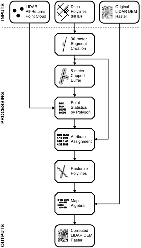
Figure 1. Workflow showing the data and processing steps for feature hydro-correction.

FIGURE 2

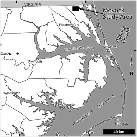
Figure 2. Study area location, Moyock, North Carolina, USA.

Ditch LIDAR Point and Line Feature Extraction

Algorithm for LiDAR Points and Hydrography Vectors

A methodology for improving topographic characterization in micro-relief settings will need to factor LiDAR data collection and post-processing techniques, as well as availability of ancillary hydrologic geospatial data availability. Illustrated in Figure 1, out approach begins with acquisition of both an all-return LiDAR point cloud (mass points) and raster DEM of the area of interest (AOI). The method does not require data from the same LiDAR repository, however, it is advisable to use data from the same acquisition mission when possible in order to avoid systematic differences in sensor and mission parameters. If using data from the same collection is not possible, one should ensure matching vertical datums between datasets. Our analysis vertically referenced data to NGVD88 and horizontally to the NC State Plane coordinate system. In addition, selection of all-return vs. BE return or similarly filtered or classified LiDAR returns should be evaluated. In this case study, mass points from all-returns were used without filtering or smoothing since the LiDAR flight campaign was across an unvegetated, leaf-off agricultural area. Generally, a further processed LiDAR collection of BE-filtered points, or a selection for BE points from a LAS dataset, would typically be utilized. In addition, a source of digitized hydrographic features at an appropriate scale can greatly reduce the processing effort for ditches. Polyline hydrography or linear feature extraction of polygonal waterbodies provides a simple set of features for classification of LiDAR points and establishing areas of focus for spatial analysis including buffers to select by location and subsequent interpolation of values and rasterization. In the US, 1:100,000 scale US Geological Survey National Hydrography Dataset (NHD), or 1:24,000 scale high-resolution NHD or similar, if available for an AOI, will be required. NHD are extensively available in the USA as a source for hydrographic geodata, and 1:100,000 NHD ditch and canal line features were used for our study. These data ensure that only the line features that should be included in processing are selected, typically NHD Flowline features with feature code (FCode) values are useful (33600, 33601, or 33602, for canal and ditch features, respectively).

Once all necessary data have been acquired and extracted, processing begins (Figure 1) by splitting the hydrographic line features into segments of appropriate length (30 m in the Moyock test) to ensure that variability is represented along the length of very long features. This can be done using a variety of feature segmentation tools (e.g., the Split tool in ArcGIS 9.x-10.x Editor toolbar or a module like v.split if using GRASS² GIS) (ESRI, 2015). Splitting the linear features into systematically spaced segments is a process termed line densification. The resulting densified line features are then buffered outward to a distance selected to best cover the width of the digitized hydrographic features (5 m in the Moyock, NC, example), without dissolving overlapping buffers and with rounded line caps. Choice of a buffer distance to select LiDAR points is inherently locally dependent upon the general spatial structure of ditches (width, in particular). The result of this analysis is a single buffer polygon feature for each segment comprising the densified hydrographic feature lines.

The output buffers from the previous step are used to extract Z-value statistics from the LiDAR all-returns point cloud point, effectively capturing elevation data from points that fall inside the small hydrographic features which are too fine to be represented in an interpolated raster grid where many other returns influence the final elevation value of each cell. This can be accomplished in ArcGIS using a Spatial Join or with a module like v.vect.stats in GRASS. The output of this step should be a set of buffer polygons with attribute fields for each statistic computed from the point cloud elevation values. Only the minimum Z-value statistic is used in our Moyock example, but other statistics could be used just as easily, depending on the desired result. The elevation statistic attributes are then transferred back to the densified hydrographic line features using another Spatial Join in ArcGIS or v.overlay in GRASS.

The hydrographic line features are next rasterized in our algorithm at the same grid resolution as the LiDAR BE DEM using the value of the chosen elevation statistic as the output cell value. The rasterized lines are combined with the original LiDAR DEM using a map algebra expression (e.g., accomplished in ArcGIS 9.x-10.x via the Raster Calculator or via r.mapcalc in GRASS). This map algebra expression simply replaces the value of the LiDAR DEM raster with the value of the rasterized line features when both rasters have a value (are not coded NULL/NODATA), effectively “burning” the line features into the original DEM with localized ditch minimum elevation attributes rather than global values. The output of this step is a hydro-conditioned LiDAR DEM which can be used for modeling or other work where a more accurate representation of fine-scale surface hydrologic features and processes is important. In the next section, this analysis process is demonstrated by comparison and illustration of improvements in hydrologic feature delineations and inundation modeling.

Canal and Ditch Buffers and Depths

A DEM and all-returns point cloud were obtained from the North Carolina Floodplain Mapping Program. Both the point clouds and BE DEM were products of the same LiDAR acquisition program. A subset of the 1:100,000-scale NHD was used as the source of digitized hydrographic features. A 30 m segmentation distance was selected to densify long linear features which were composed of few segments. The segments were buffered using a 5 m buffering distance, no dissolve, and rounded line caps. The 5 m buffering distance was chosen since most of the ditches in the AOI would fit within a buffer of this dimension.

To assess the validity of the buffer and its performance with proximal LiDAR last-return points as elevation estimation for ditches, we extracted elevation statistics from the point cloud for each buffer and then assigned to the line segment from which the buffer was derived. Figure 3 depicts a single canal extraction as an example of this exploratory phase. The Guinea Mill Canal drains an extensive former pocosin vegetation of peaty muck soils approximately 5 km south of Moyock above the Northwest River. This canal was historically dug to connect feeder ditches from farmland for drainage and subsequent production (now primarily corn, cotton, and soybeans). This large canal also provided a transportation route similar to other large ditches in the region. Figure 3 illustrates in the map (Figure 3A) the linear extent of a subset of the area used for evaluating the ditch lines and associated buffer point clouds. We calculated the point cloud elevation values within an equival interval step classification within distance bands (internal buffers) of the ditch centerline. In addition, we estimated a range and ordinary least-squares best fit regression to assess the representativeness of ditch point mean elevations with distance from the ditch centerline as in Figure 3C. The ditch point cloud and buffer analysis was iterated for all ditch segments in the intensive study area, which included a range of canals, feeder ditches, and stormwater drainage ditches surrounding the Town of Moyock. This analysis was used to guide a selection of buffer distance of 5 m, which represents a local threshold on ditch cross-sectional radius. Buffers beyond this distance would inevitably have included non-ditch elevation values and potentially captured features unrelated to the actual ditches.

FIGURE 3

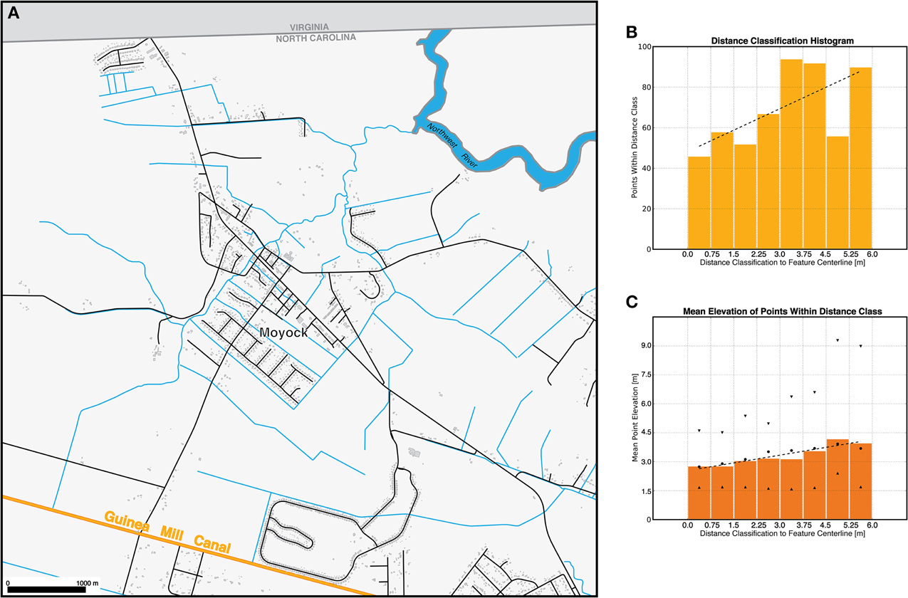
Figure 3. Map inset (A) depicts a subset area of Moyock including all ditches, canals, and riverine hydrography (blue), roads (black), and buildings (grey) with the large Guinea Mill Canal highlighted to illustrate subsequent LiDAR point and buffer analyses; inset chart (B) histogram shows the number of points (y-axis) vs. multiple buffer distances of the Guinea Mill Canal centerline (x-axis), an analysis that was conducted on all ditched features; and the chart (C) illustrates the elevation variation of LiDAR points with distance from the centerline of Guinea Mill Canal, highlighting a best-fit OLS regression relationship used in selecting an optimal buffer distance to preserve minimum elevation for attributing the ditch.

Following the outline of Figure 1, utilizing the mean ditch point elevation values within the buffer for each segment, the depth attribute were created for the ditch lines. These newly attributed hydrographic line features were then rasterized at a 6 m resolution (co-registered to the DEM) using the minimum elevation statistic to determine the cell values, resulting in a raster with floating-point values in cells containing ditches and NODATA in all other cells. Finally, a map algebra expression was used to combine the values from this raster with the original DEM, overwriting the value of the DEM with that of the rasterized ditches where a valid ditch depth could be determined.

The hydro-conditioned output DEM, now containing more extensive ditches, was next used as one input to a series of flood inundation scenarios based on a hydro-connected bathtub inundation model. This modeling approach uses a cost-distance function to enforce adjacency (Queen's case, or D8 flow direction) in addition to elevation thresholding to determine potential inundation. The approach eliminates potential isolated inundation areas (only affected by rainfall, watershed runoff, or groundwater elevation) as cells of the raster are contagiously tested from a source flood zone raster (typically an existing bay, estuary, or permanently flooded riverine waterbody where floodwaters could backfill a drainage). In addition, the new hydro-conditioned DEM was saved for quantitative and visual analysis (Figure 4).

FIGURE 4

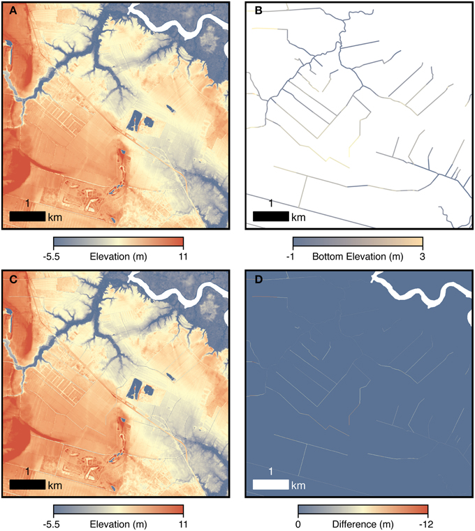
Figure 4. Illustration of pre- and post-hydrologic correction with inset (A) original DEM, (B) extracted stream and ditch line network as minimum point cloud buffer calculations attributed to raster cells, (C) hydro-conditioned DEM, and (D) elevation differences in the ditch network.

Inundation Model and Visualization

To robustly evaluate the potential changes in the extent of inundation, we flooded the hydro-conditioned DEM with a “bathtub” type model after the method of Poppenga and Worstell (2015) to spatially capture gross changes in potential flood areal extent with different inundation levels. This algorithm was implemented using a cost distance function and enforcement of Queen's case connectivity (D8). A script implemented the inundation algorithm for more than 100 successive levels of inundation in order to also generate individual maps (e.g., Figure 5) as well as an animation of inundation that could contrast the extent of inundation of a BE DEM vs. the new hydro-conditioned product. Rasters for each inundation zone were also stored for future hypsometric analysis.

FIGURE 5

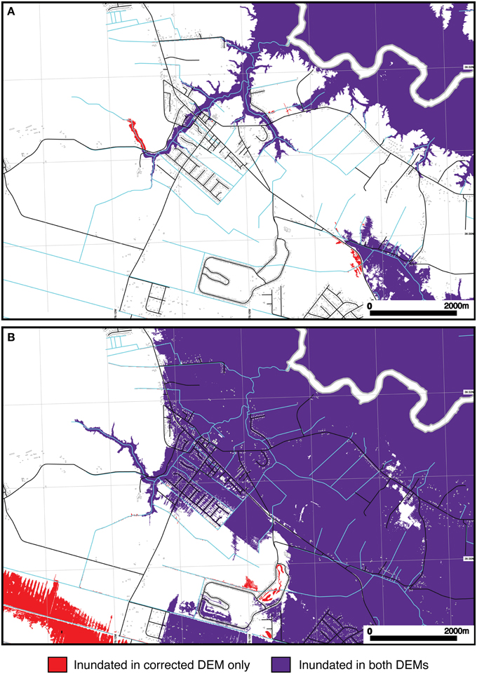
Figure 5. Maps comparing the areas inundated in two source connectivity ensured hydrologic inundation scenarios with both the original and hydro-corrected DEMs. (A) Base level scenario with water surface at mean sea level; (B) 2.75 m water rise scenario, illustrating areas in red where the hydro-conditioned DEM highlights potential upland inundation from a storm surge that would be omitted in a raw bare earth DEM without hydro-correction and -conditioning.

Ditch and Canal LiDAR Depth Difference

DEMs of difference were also developed by raster overlay and subtraction to create maps of the current ambient water level during regular, non-flooding conditions. In addition, we extracted the raster network of ditch elevations and the differences to assess the degree and potential elevation and volumetric differences between the baseline BE DEM and the hydro-conditioned DEM.

Hydro-conditioning and Subwatershed Delineations

In a final examination of the spatial impacts of ditches in drainage delineation, we implemented a watershed delineation algorithm using derived flow direction, accumulation, and arbitrary subwatershed threshold area. This analysis was chosen to explore potential contrasts in subwatershed delineation using the BE DEM vs. hydro-conditioned DEM. Since many coastal areas lack fine-scale subwatershed delineations, this step would be informative of the reliability of potential basins resulting from alternative characterizations of flow.

Results

The hydro-corrected and conditioned output DEM containing ditches was one input to a series of flood inundation scenarios based on a hydro-connected bathtub inundation model. This modeling approach used a cost-distance function to enforce adjacency (Queen's case, or D8 flow direction) in addition to elevation thresholding to determine potential inundation. The approach eliminates potential isolated inundation areas (only affected by rainfall, watershed runoff, or groundwater elevation) as cells of the raster are contagiously tested from a source flood zone raster (typically an existing bay, estuary, or permanently flooded riverine waterbody).

Ditch and canal buffer results (Figure 3) prompted the heuristic selection of a 5 m buffer threshold. The Guinea Canal example in Figure 3 illustrates a wider canal example, wherein the 5 m buffer captures all ditch points within the point cloud. In addition, this case and others assessed also corroborated the use of symmetrical buffering. While a surrogate for stream order could potentially be developed, wherein variable buffers are applied or even actual ditch widths and cross-sectional areas are delineated from the point clouds, this step simply affirmed the use of a simple buffer.

The methodology was similarly affirmed in derived DEMs of differences and the extracted ditch surface values in the resulting raster (Figure 4). Figure 4B illustrates the depths of ditches using the minimum point cloud value from within buffer segments. This clearly isolates the ditches vs. the surrounding terrace surfaces as well as illustrates hydrologic continuity in descending elevations “downstream” through the ditch network to the Northwest River. Elevation differences between the original DEM and the ditch elevations after hydro-conditioning in Figure 4D also highlight patterns of moderate depth changes, showing that the ditches after conditioning exhibit significant, obvious changes in elevation. Although volumetric analyses and potential implications for runoff and sediment of pollutant transport or capture could be analyzed, this figure elegantly captures significant geomorphic differences that could facilitate later analysis, hydrologic modeling, and water management.

The areal extent of inundation zones comparisons in Figure 5 (and Supplementary Video 1) present evidence for extensive differences in the extent of potential flooding between a baseline BE DEM and hydro-conditioned DEM. Figure 5A depicts a still-water elevation outside of flood conditions, yet shows a slight extension of the inundated area across a road, as a result of a ditch segment crossing a road and capturing a culvert. In addition, Figure 5B shows an even more significant extent of potential flooding (red) after hydro-conditioning, wherein the Guinea Canal floods feeder ditches in a 2.75 m flood scenario. These grids illustrate agreement (purple) and potential error of omission (red) in the case of the baseline BE DEM. The red areas in Figure 5 are inundated because of the hydrologic connectivity that the conditioning process has implemented on the new DEM. Hence, inundation models (even a bathtub) seeks to fill the connected rasters that meet a minimum elevation threshold, resulting in a contagious diffusion and new flowpaths that are not floodable in the baseline DEM. Such errors of omission are an artifact of the resolution of the BE DEM, the lack of representation of ditches and canals, and random errors with positive elevation bias, or omission of structures such as culverts and related control structures.

Finally, the subwatershed delineations (Figure 6) illustrate that fien-scale ditches affect the area thresholding and along-stream segmentation of basins. Although many subwatershed were in agreement (purple), the hydro-conditioned DEM generated more watershed delineations capturing drainage areas mediated by ditch and canal controls. Since hydrology this coastal area is overwhelmingly controlled by ditch and canal structures, these subwatersheds are potentially new improvements for land management, including agricultural drainage, stormwater runoff management, nutrient and sediment flows, and even retaining water in uplands for pocosin vegetation management and forest and peat fuel control. The stark differentiation of subwatershed boundaries in the test area of Figure 6 suggests the need for additional, rigorous analysis, and comparison to field-scale hydrologic monitoring such as the NC Streambed Mapping Project (NCSMP, 2006). Nonetheless, improving the representation of ditches thus affords finer, more accurate basin representations. This performance warrants further investigation but has the potential to significantly improve low-relief coastal LiDAR applications. For instance, may coastal areas with interspersed agricultural and residential development experience periodic high-discharge stormwater runoff events. Better representation of functional subwatersheds could improve the targeted application of best management practices (BMPs) such as retention ponds, prescription of discharge and flow capacities for culverts, or selection of low-impact development alternatives (LIDs) such as vegetated swales. In addition, these subwatersheds can be derived in a semi-automated fashion as illustrated here at low cost and serve planning and permitting applications as a guide to potential stormwater permitting or fee schedules based on runoff and impervious surface cover as a function of basin and not simply parcel-based.

FIGURE 6

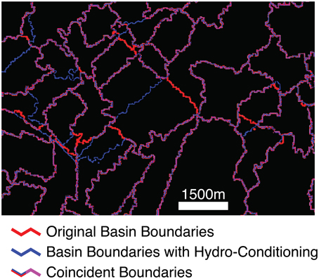
Figure 6. Comparison of watershed sub-basin boundary delineations without ditches (red), with ditches (blue), and overlaid agreement (purple).

Discussion and Conclusion

Our key findings pertain to the opportunity to efficiently improve coastal LiDAR DEMs through the inclusion of hydro-conditioning correction processes. This analysis shows the visual and hydrologic improvements afforded by mapping and then attributing the linear ditch (or stream segments) typical of DEM hydro-correction. In the USA, extensive high-resolution NHD hydrography data provide a starting point for automating the process. In other regions, mapping ditches may require aerial orthophotography or ultra high-resolution optical satellite data. Attributing the ditch features with representative elevation values from a buffer analysis of the LiDAR point cloud has indeterminate error in this study, yet still the results illustrated in Figures 3–5 depict a variety of evident and consistent visual improvements. The hydro-conditioned DEMs lack blockages evident in downslope runoff or flow accumulation models, do not exhibit pits or sinks as frequent artifacts in interpolated BE DEMs, and also show improvement in the lessening of omission errors of potential upstream surges or floods.

Additional significance of this work relates to concomitant improvements in feature extraction techniques in remote sensing even as LiDAR data improves vertical and horizontal data accuracy. Object-Oriented Image Analysis (OBIA), for instance, can provide a means for more automated and reduced cost ditch mapping. Synthesis of ditches and GIS data in pre-processing of LiDAR data will also provide for the hydro-conditioning in a priori phases of mapping projects. In low-relief environments, such features and artificial structures are vital to resource and hazards management. Planning and scenario analysis of coastal hydrologic projects, coastal hazards management, and agricultural point and non-point source pollution modeling can make use of these improvements in coastal DEMs as well. In coastal NC, these improved DEMs are seeing greater application to simulate hydrologic management practices and inform local agricultural, residential, and transportation plans. They are beginning to be used for simulating the effects of storm surge inundation, riverine flood back-filling of tributaries, site selection of coastal hydrologic restoration structures, and informing policies for regulating stormwater runoff.

Although much of the Earth lacks LiDAR DEM data for these crucial applications, this paper aims to inform potential users and procurers of LiDAR data that low-cost mapping and geospatial analysis techniques are increasingly available to capitalize on LiDAR data in even the most low-relief environments. The geospatial, geomorphic, and hydrologic research communities have made great strides to document the accuracy, error, and improvements possible for coastal LiDAR. Further research on hydro-correction overall, and hydro-enforcement and –conditioning in particularly is likely to proceed at an accelerated rate as sea-level rise and climate change further threaten extensive coastal resources and communities. More intensive investigation of scale-dependence of landforms and derivation of practical tools (e.g., web-based analytical tools that do not require extensive data downloads) are warranted. These techniques and tools will amplify the power of LiDAR and encourage additional monitoring of changes in dynamic coasts (e.g., shoreline change), regulation of environmental practices (e.g., ditching), and synergy with modeling of environmental stressors and pollutants that flow through coastal landscapes and estuaries.

Conflict of Interest Statement

The authors declare that the research was conducted in the absence of any commercial or financial relationships that could be construed as a potential conflict of interest.

Acknowledgments

The authors wish to thank the staff of the NC Floodplain Mapping Program, Office of Geospatial Technology Management, for providing data and technical assistance. Mr. Ben Woody of Currituck County Environmental Planning Office encouraged the early exploration of coastal watershed delineations. Early phases of this work were also supported by the Renaissance Computing Institute (RENCI) of the University of North Carolina at Chapel Hill and the Cooperative Institute for Coastal and Estuarine Environmental Technology (CICEET) at the University of New Hampshire. We also thank the two reviewers for corrections and improvements to the original manuscript.

Supplementary Material

The Supplementary Material for this article can be found online at: https://www.frontiersin.org/article/10.3389/feart.2015.00072

Video 1. An animation is included depicting a storm surge simulation for the vicinity of Moyock, North Carolina, illustrating the improvements of the hydro-conditioned DEM. The animation increments a step-wise 30.5 cm increment and shows the results of a inundation for a bare earth DEM (purple) vs. conditioned (purple AND red areas inundated) as in Figure 4.

Footnotes

1 ^US Geological Survey (2007). National Hydrography Dataset. Available online at: http://nhd.usgs.gov (Accessed February 22, 2010).

2 ^GRASS Development Team (2015). Software, Version 7.0. Open Source Geospatial Foundation. Geographic Resources Analysis Support System (GRASS). Available online at: http://grass.osgeo.org

References

Allen, T. R. (2014). “Advances in remote sensing of coastal wetlands: LiDAR, SAR, and object-oriented case studies from North Carolina,” in Remote Sensing and Modeling: Advances in Coastal and Marine Resources, eds C.W. Finkl and C. Makowski (Boca Raton, FL: CRC Press), 405–428.

Barnes, J. (2001). North Carolina's Hurricane History. Chapel Hill, NC: UNC Press.

Google Scholar

Brock, J. C., and Purkis, S. J. (2009). The emerging role of LiDAR remote sensing in coastal research and resource management. J. Coast Res. 53, 1–5. doi: 10.2112/SI53-001.1

CrossRef Full Text | Google Scholar

Brock, J. C., Wright, C. W., Clayton, T. D., and Nayegandhi, A. (2004). LIDAR optical rugosity of coral reefs in Biscayne National Park, Florida. Coral Reefs. 23, 48–59. doi: 10.1007/s00338-003-0365-7

CrossRef Full Text | Google Scholar

Environmental Systems Resource Institute (ESRI) (2015). ArcMap 10.3.1. Redlands, CA: ESRI. Available online at: http://www.arcgis.com

Floodplain Mapping Program North Carolina Division of Emergency Management (NCFMP) (2002). NC Floodplain Mapping: Pasquotank Basin; LIDAR Bare Earth Derived 3D Breaklines. Raleigh, NC: GIS World.

Gallant, J. C., and Wilson, J. P. (2000). “Primary topographic attributes,” in Terrain Analysis: Principles and Applications, eds. J. P. Wilson and J. C. Gallant (New York, NY: Wiley and Sons), 51–86.

Google Scholar

Hladik, C., and Alber, M. (2012). Accuracy assessment and correction of a LIDAR-derived salt marsh digital elevation model. Remote Sens. Environ. 121, 224–235. doi: 10.1016/j.rse.2012.01.018

CrossRef Full Text | Google Scholar

Hutchinson, M. F., and Gallant, J. C. (2000). “Digital elevation models and representation of terrain shape,” in Terrain Analysis: Principles and Applications, eds J. P. Wilson and J. C. Gallant (New York, NY: Wiley and Sons), 29–50.

Krabill, W. B., Wright, C. W., Swift, R. N., Frederick, E. B., Manizade, S. S., Yungel, J. K., et al. (2000). Airborne laser mapping of Assateague National Seashore Beach. Photogramm. Eng. Remote Sens. 66, 65–71. Available online at: http://eserv.asprs.org/PERS/2000journal/jan/2000_jan_65-71.pdf

Maune, D. F. (2007). “DEM user requirements,” in Digital Elevation Model Technologies and Applications: The DEM Users Manual, 2nd Edn., ed D. F. Maune (Bethesda: American Society for Photogrammetry and Remote Sensing), 449–473.

Maune, D. F., Kopp, S. M., Crawford, C. A., and Zervas, C. E. (2007). “Introduction,” in Digital Elevation Model Technologies and Applications: The DEM Users Manual, 2nd Edn., ed D. F. Maune (Bethesday: American Society for Photogrammetry and Remote Sensing), 1–35.

Mitasova, H., Overton, M., and Harmon, R. S. (2005). Geospatial analysis of a coastal sand dune field evolution: Jockey's Ridge, North Carolina. Geomorphology 72, 204–221. doi: 10.1016/j.geomorph.2005.06.001

CrossRef Full Text | Google Scholar

North Carolina Floodplain Mapping (NCFMP) (2015). Partners participating in the NC Cooperating Technical State (CTS) Program. Available online at: http://www.ncfloodmaps.com/partners.htm (Accessed August 31, 2015).

North Carolina Streambed Mapping Project (NCSMP) (2006). ISSUE 3: The Western North Carolina 6-Acre Drainage Area Calculation. Available online at: http://www.ncstreams.org/

Poppenga, S. K., Gesch, D. B., and Worstell, B. B. (2013). Hydrography change detection—the usefulness of surface channels derived from LiDAR DEMs for updating mapped hydrography. J. Am. Water Res. Assoc. 49, 371–389. doi: 10.1111/jawr.12027

CrossRef Full Text | Google Scholar

Poppenga, S. K., and Worstell, B. B. (2015). Evaluation of airborne Lidar elevation surfaces for propagation of coastal inundation: the importance of hydrologic connectivity. Remote Sens. 7, 11695–11711. doi: 10.3390/rs70911695

CrossRef Full Text | Google Scholar

Poulter, B., and Halpin, P. N. (2008). Raster modelling of coastal flooding from sea-level rise. Int. J. Geogr. Info. Sci. 22, 167–182. doi: 10.1080/13658810701371858

CrossRef Full Text | Google Scholar

Raber, G. T., Jensen, J. R., Hodgson, M. E., Tullis, J. A., Davis, B. A., and Berglund, J. (2007). Impact of Lidar nominal post-spacing on DEM accuracy and flood zone delineation. Photogramm. Eng. Remote Sens. 73, 793–804. doi: 10.14358/PERS.73.7.793

CrossRef Full Text | Google Scholar

Stockdon, H. F., Doran, K. S., and Sallenger, A. H. (2009). Extraction of LiDAR-based dune-crest elevations for use in examining the vulnerability of beaches to inundation during hurricanes. J. Coast Res. 35, 59–65. doi: 10.2112/SI53-007.1

CrossRef Full Text | Google Scholar

Webster, T. L., Forbes, D. L., Dickie, S., and Shreenan, R. (2004). Using topographic lidar to map flood risk from storm-surge events in Charlottetown, Prince Edward Island, Canada. Can. J. Remote Sens. 30, 64–76. doi: 10.5589/m03-053

CrossRef Full Text | Google Scholar

Yang, J., and Artigas, F. J. (2010). “Mapping salt marsh vegetation by integrating hyperspectral and LiDAR remote sensing,” in Remote Sensing of Coastal Environments, ed J. Wang (Boca Raton, FL: CRC Press), 173–190.