Snow in a Very Steep Rock Face: Accumulation and Redistribution During and After a Snowfall Event

1. Introduction

Snow in rock faces influences the occurrence of permafrost and thus affects the stability of steep slopes and rockfall danger (Gruber et al., 2004; Luetschg et al., 2008; Haberkorn et al., 2015). Snow in very steep slopes is important for avalanche danger forecasting because snow avalanches often form in steep terrain interspersed with rock (Schweizer et al., 2003) and it contributes to runoff in spring (Anderton et al., 2002; Lehning et al., 2006). Studying snow in rock faces can also increase understanding of snow and precipitation distributions in general, e.g., altitudinal gradients of snow amounts (Grünewald and Lehning, 2011).

Many studies suggest that the amount of snow is inversely proportional to the slope angle and that no snow accumulates (permanently) above a certain critical angle. Blöschl and Kirnbauer (1992) observed that snow covered area (SCA) decreased with increasing slope angle and that terrain steeper than 60° was usually snow-free due to gravitational effects (avalanching) and wind. Winstral et al. (2002) and Gruber Schmid and Sardemann (2003) assumed that slopes steeper than 50° accumulate little or no snow. Machguth et al. (2006) modeled avalanching by removing most snow from areas steeper than 60°. Blöschl et al. (1991) reported critical angles between 45 and 70° and attributed the large scatter to differences in climatic conditions. In an older study concerning the Swiss Alps, a critical angle of 50° was observed (Witmer, 1984). The spatial resolution, i.e., the grid size of the digital elevation model, in these studies varied between 5 and 90 m. Generally, it appears that the critical angle increases with decreasing grid size. However, Blöschl et al. (1991) maintain that the effect of climate is more important than that of the grid size.

TLS, i.e., terrestrial laser scanning (Heritage and Large, 2009), was first used to acquire snow depth data by Prokop (2008) and Prokop et al. (2008). Wirz et al. (2011) used TLS to study the distribution of snow in a rock face. They measured the snow depth and snow depth changes with a spatial resolution of 1 m and compared the results to measurements in gentler terrain in the vicinity. The snow depth and SCA were lower in the rock face than in the gentler, flatter terrain. The spatial pattern of snow depth was consistent in time while patterns of snow depth changes depended to some degree on the weather conditions during the snowfalls. Terrain-wind interactions were hypothesized to be primarily responsible for the observed snow depth distribution. The influence of slope angle remained unclear. The correlations between steepness and snow depth and between steepness and snow depth change were weak, there was no general decrease of snow depth with increasing slope angle. Snow was observed to accumulate in areas up to 80° steep. Haberkorn et al. (2015) measured the snow distribution in two extremely steep rock faces with a resolution of 0.2 m. Their focus was on the influence of the snow cover on the thermal regime of rock. They observed no decrease of snow depth with increasing slope angle in terrain up to 70° steep.

Wirz et al. (2011) studied the evolution of the snow cover in the rock face over a complete winter at a time scale (time interval between TLS measurements) of one to several weeks. In contrast, we concentrated on a single snowfall event and captured it with a very high spatial and temporal resolution (time scale: days). Furthermore, the quality of the snow depth data in the study of Wirz et al. (2011) was significantly lower than the quality achieved in gentle terrain. Grünewald et al. (2010) compared the TLS snow depth data to tachymetry measurements (= accuracy) and found a standard deviation of less than 5 cm. Wirz et al. (2011), on the other hand, quantified the precision. Repeatability measurements showed a standard deviation of around 20 cm, reproducibility tests had standard deviations of about 38 cm. The aims of this study are therefore twofold: first, to improve data quality by specifically adapting the postprocessing procedure to rock faces and second, to obtain information on the accumulation and redistribution of snow in extremely steep terrain.

Section 2 describes the acquisition and postprocessing of the data and ends with a subsection on data quality. The results are presented and interpreted in Section 3 and are discussed in Section 4.

2. Acquisition and Processing of Data

2.1. Measurement Location

The north-east face of the Chlein Schiahorn (henceforth just called Schiahorn) is very steep and rough. The average slope angle is 50°. More than 25% of the area is steeper than 60° and 11% is steeper than 70°. The elevation of the rock face ranges from 2300 to 2600 m a.s.l. (Figure 1). The scan position was chosen in consideration of the range, the view direction and avalanche danger. The range to the rock face should be as small as possible and the view direction should be as close to perpendicular to the rock face as possible. The chosen position is easily accessible by ski due to the proximity of the Parsenn skiing area. The range varies between 200 and 600 m. The four reflectors (circular, reflective foil targets) were installed on fixed structures and rocks. They were used to georeference (register) the scans (El khrachy, 2008; Revuelto et al., 2014a).

FIGURE 1

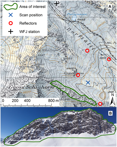
Figure 1. (A) Map of the measurement location showing the rock face, the scan position and the reflector locations. The map also shows the location of the meteorological reference station Weissfluhjoch (WFJ). (B) View of the rock face from the scan position. The extent of the area of interest is sketched in approximately. The Schiahorn is located in eastern Switzerland just to the north of Davos. Base map reproduced by permission of swisstopo (JA100118).

2.2. Data Collection

The data acquisition closely followed the procedure described by Wirz et al. (2011) and Grünewald et al. (2010) and was carried out with the same terrestrial laser scanner (Riegl LPM-321). An important instrument property is the beam divergence (0.8 mrad for the LPM-321). This angle describes how the diameter of the laser beam increases with distance and influences the size of the laser footprints on the rock face (Deems et al., 2013). The beam divergence limits the angular resolution. Lichti and Jamtsho (2006) derived the optimal sampling interval to be 86% of the beam divergence. El khrachy (2008), on the other hand, suggests to avoid footprint overlap. This infers an optimal sampling interval equal to the beam divergence. We used an angular increment of 0.045°, which is slightly smaller than the beam divergence. The reflectors were rescanned approximately every hour to account for the limited stability of the scanner setup (Prokop, 2008; Revuelto et al., 2014a). In the end, the complete rock face was scanned in about 15 min with a correspondingly coarser resolution and images of the rock face were acquired by a digital camera installed on the TLS. The data set of each measurement day consists of slightly overlapping fine scans (between three and five), the coarse scan and the images.

The rock face was scanned five times in winter: once before the snowfall (21 March 2014) and four times after the snowfall (25, 27, 28 March and 1 April). A summer scan without snow was acquired on 18 August 2014.

2.3. Weather Conditions

The weather on 21 March was sunny and mild with air temperatures between −2 and 4°C. The snowfall event occurred between 22 and 24 March. Most of the 55 cm of fresh snow fell on 23 and 24 March. From 25 March until 1 April it was sunny again and increasingly warm. Temperatures ranged between −16 and −3°C on 25 March and between −1 and 8°C on 1 April. During the whole period, there were only weak winds (mean wind speeds < 6 ms⁻¹, max. wind speeds < 11 ms⁻¹). The predominant wind direction was south-east on 21 and 22 March and north-west on 23 and 24 March. After 25 March, the wind direction was variable and mean wind speeds decreased to below 3 ms⁻¹ (max. wind speeds < 8 ms⁻¹). All meteorological data were taken from the automatic station Weissfluhjoch (WFJ), which is at a distance of 1.5 km from the Schiahorn (see Figure 1A). The station is located in a slope with an average aspect of south-east, but the terrain around the station is flat. The elevation of the station is 2540 m a.s.l. The temperature at WFJ in March 2014 was 2.7°C higher than the long-term average (1981–2010). Regarding snow depth and new snow, March 2014 was below average. The long-term average snow depth is 192 cm. In March 2014 the mean snow depth was 152 cm. For new snow, the numbers are 137 and 69 cm.

2.4. Postprocessing

While the process of data acquisition was very similar to previous studies, the postprocessing was modified substantially. Wirz et al. (2011) noted that TLS performance deteriorates in the rough terrain of a rock face. In our opinion, the main reason for this deterioration is not the roughness, but the steepness of a rock face. Snow depth is the magnitude of the snow cover in the vertical direction (Fierz et al., 2009). The extreme slope angles lead to a high sensitivity of snow depth to misalignments between the compared scans (registration errors). The errors may be small in the horizontal but in steep terrain, they can quickly amplify in the vertical. In fact, the vertical error is the horizontal error multiplied by the tangent of the slope angle, which tends to infinity as the slope angle approaches 90°. Snow thickness, on the other hand, is the magnitude of the snow cover perpendicular to the surface (Fierz et al., 2009). The registration errors are not amplified in steep terrain because the slope angle is taken into account in the calculation of snow thickness. TLS scans are usually analyzed by viewing them from the top, e.g., in a GIS software. This can be problematic because extremely steep terrain is barely visible from this direction. Such terrain can be analyzed in much more detail by rotating the scans and viewing them from the front. This also ensures that the point cloud does not overlap in vertical and overhanging areas and makes the interpolation (triangulation) much easier. The Schiahorn was viewed from the north-east and downwards at 30°. This direction was chosen based on the averages of aspect and slope angle. It is the optimal view direction because it is perpendicular to the “average rock face.” All measures of length or surface area below were calculated in a plane perpendicular to this view direction. Figures 2, 3, 5, 6, 10 show the rock face from this direction. This orientation is similar to the view in Figure 1B.

FIGURE 2

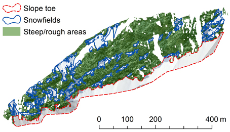
Figure 2. Division of the rock face into three subareas: “slope toe,” “snowfields” and “steep/rough” areas. The orientation of the rock face is similar to the view in Figure 1B.

FIGURE 3

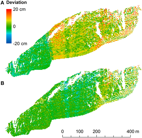
Figure 3. Errors between fine and coarse scans (A) before and (B) after MSA. (A) The boundary between two of the fine scans is visible as a sharp transition of the error. (B) MSA reduced the registration errors (systematic error). Note, however, that there are still some spatial patterns in the errors. The case of 21 March is shown. The orientation of the rock face is similar to the view in Figure 1B.

After applying the usual corrections and filters (atmospheric and geometric corrections, remove-isolated-points and octree filters, e.g., Prokop, 2008 or Wirz et al., 2011), the different fine scans of one measurement day were registered to each other using the reflectors. Registration is the process of transforming different scans to a common coordinate system. The assembled fine scans were then compared to the coarse scan to check the quality of the registration. The registration could often be improved with a method called Multi Station Adjustment (MSA). This extension of the software RiScanPro uses an iterative closest points (ICP) algorithm to adjust different scans to each other (Kenner et al., 2011). We used it to adjust the fine scans to the coarse scan. The best results were achieved by considering triangulated surfaces (interpolations) in addition to the reflectors. That way, every triangle becomes a tie point like a reflector. MSA was also applied to improve the registration between the different measurement days. Only unchanged parts of the surface can be used for MSA. Between two measurement days, these are the areas that were snow-free on both days. The snow-free rock surfaces were filtered out, triangulated and adjusted to each other. The adjustment of the fine scans to the coarse scan, on the other hand, was done using the complete surface.

The snow thickness changes were calculated in this MSA-corrected coordinate system and were then transformed into the Swiss coordinate system CH1903 and rotated to be viewed from the front. The snow-free areas were neglected in the calculation of averages to reduce noise. Snow and rock can be distinguished based on RGB color information (Wirz et al., 2011). Cells were classified as snow if they had a blue band value higher than 190 or if they had a red/blue ratio higher than 1.1 and a blue band value higher than 100. Furthermore, snow patches with a surface area below 1 m² were neglected as well and gaps in the point cloud larger than 1.2 m were considered as measurement shadows and were not interpolated. The rasters of snow thickness change were created in ArcGIS with a cell size of 0.5 m. This corresponds to the average point spacing in the original point cloud. The grid size should be similar to that value to minimize smoothing and scaling concerns (Deems et al., 2013).

Winter and summer slope angles were calculated. The winter slope angle was based on the surface of 21 March and is relevant for the snow thickness change. The summer slope angle was based on the surface of 18 August and corresponds to the steepness of the underlying terrain. The correlation between snow thickness changes and topographic parameters may depend on the resolution of the latter (Blöschl, 1999; Deems et al., 2006). Wirz et al. (2011) tested different resolutions but did not find significant differences. We used a resolution of 0.5 m for the slope angle rasters.

The rock face was divided into three subareas (Figure 2). The extent of the “slope toe” was defined manually based on the orthophoto (undistorted, georeferenced image) of 25 March. The “slope toe” is the area below the lowest rock areas, i.e., below the actual rock face. This boundary was very clear (Figure 1B), such that this method should be applicable to other study sites. If the “slope toe” extent is not evident, it probably makes more sense to only use the two other subareas. The “snowfields” were defined based on the snow/no snow classification (see above) of 25 March. “Snowfields” are snow-covered areas with a surface area above 90 m² and a area/perimeter ratio above 1.3. The second condition removes areas with extremely complicated and distorted shapes. The “steep/rough” areas encompass the rest of the rock face. This subarea contains many small snow patches and most of the snow-free areas.

2.5. Data Quality

The software RiScanPro calculates the standard deviation between tie points used for registration. These values are one way to analyze data quality. For the registration of the different fine scans of one measurement day without MSA, this calculation only includes the reflectors. The average standard deviation for all measurement days in winter was 0.6 cm. Despite this small value, there were systematic errors in the registration (Figure 3A). After MSA, the average standard deviation between the tie points was 2 cm. Note that this value now includes every triangle in addition to the reflectors. In spite of this value being higher than 0.6 cm, MSA improved the registration (see Figure 3B and below). The standard deviation of the MSA-corrected registration between the different measurement days was 1.8 cm.

A better way to analyze data quality is to directly quantify the accuracy and precision of the snow thickness data. The accuracy could not be calculated because no independent measurements were available. However, the precision (repeatability and reproducibility) was measured. The repeatability was tested by comparing the fine scans to the coarse scan of each measurement day. Note that this is an approximation of repeatability because the spatial resolution of the compared scans was different. For each measurement day, the mean error (offset, systematic error) and the standard deviation of the error was calculated. The average of the absolute values of the mean errors $\overline{\left|\mu \right|}$ was 0.5 cm, the average of the standard deviations $\bar{\sigma }$ was 3.7 cm. The effect of MSA was quantified for the measurement of 21 March. Before MSA, the statistics were μ = 2.6 cm and σ = 5.8 cm (Figure 3A). The application of MSA reduced these values to μ = −0.5 cm and σ = 3.6 cm (Figure 3B). Therefore, MSA clearly improved the registration and the quality of the data. The application of MSA can be problematic and even increase errors if the used areas are wrongly assumed to be unchanged. In case of the registration of the fine scans to each other, this could happen if an avalanche occurs between the different scans.

The reproducibility was tested by comparing the rock surfaces between different measurement days. We compared subsequent scans to each other and the last scan (1 April) to the first scan (21 March). The average statistics for the reproducibility tests were $\overline{\left|\mu \right|}=0.3$ cm and $\bar{\sigma }=4.6$ cm. The distributions are such that more than 90% of the values are on average contained in the interval ±7 cm. This average includes repeatability and reproducibility tests. The precision of the snow thickness measurements is thus an order of magnitude higher than the precision of the snow depth data in Wirz et al. (2011). Note, however, that the values given here represent the best case scenario because the same areas were used for MSA and the comparison. But even the standard deviation without MSA (5.8 cm) is lower than the value given by Wirz et al. (2011) (20.3 cm). This suggests that the improvement is mostly due to the use of snow thickness instead of snow depth.

The error of the snow thickness measurements has two components. The error introduced during the acquisition and the error introduced during the postprocessing. The acquisition error depends on the instrument and increases with the range, the incidence angle (angle between laser beam and target surface normal) and the roughness of the target surface (Deems et al., 2013). Because it depends on the target surface, the acquisition error is not constant across the rock face (see Figure 3B). Other acquisition error sources include edge effects and laser penetration into the snow surface. The latter effect is generally negligible (Prokop, 2008; Deems et al., 2013). Edge effects (Boehler et al., 2003) appear when the laser beam (due to the beam divergence) hits more than one target. This may happen at the edges of rock ledges, for example. The postprocessing error is caused by errors due to the interpolation of the point clouds and the registration error.

It appears that the dominant component is the registration error. All other errors are expected to be similar between this study and that of Wirz et al. (2011) because we used the same instrument and methods. The targets also had similar properties. This leaves the improvement of the postprocessing as the main cause for the better precision in this study.

3. Results and Interpretation

3.1. Spatial Distribution of Snow Thickness and Snow Thickness Change

The subareas were compared in terms of winter slope angle, snow thickness change during the snowfall event (ΔDS) between 21 and 25 March and snow thickness (DS) on 25 March (Figure 4). The “slope toe” is the flattest subarea with slope angles limited to a fairly small range around 40° (Figure 4A). The slope angles in the other two subareas cover a very wide range of values, the steepness of the terrain is highly variable. The two ranges overlap for the most part but the slope angles are nonetheless significantly higher in the “steep/rough” areas than in the “snowfields.” ΔDS and DS were highest in the “slope toe,” lowest in the “steep/rough” areas and reached intermediate values in the “snowfields” (Figures 4B,C). The variability of ΔDS and DS followed the same pattern. There are negative values of ΔDS in all three subareas. Snow appears to have been ablated in some places. There are also some negative values of DS, especially in the “snowfields.” There were several outliers with DS between −2 and −1 m. It could be shown that these extreme values are due to hikers in the summer scan (a trail passes through the area of interest). The less extreme negative values are mostly located at the edges of rock ledges and could be caused by edge effects. These values also appeared mostly in areas where the measurement noise was above average due to increased range and incidence angle (rightmost part in Figure 3B). Rockfall could also be a reason for negative snow thicknesses. Overall, less than 2‰ of the values were below −0.15 m. The effect of these values on the results are small. Excluding them would change the average snow thickness by less than 2 mm. Flatter terrain accumulated more snow during this snowfall event and also during the complete winter. Pearson's correlation coefficient is r = −0.61 between ΔDS and the winter slope angle and r = −0.59 between DS and the summer slope angle.

FIGURE 4

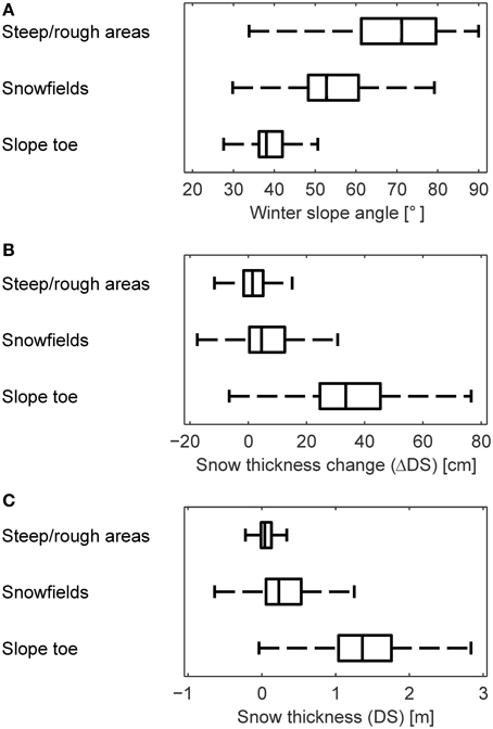
Figure 4. Comparison of the subareas with regard to (A) winter slope angle, (B) snow thickness change during the snowfall, and (C) snow thickness on 25 March. The flatter the subarea, the more snow was accumulated and the higher was the total snow thickness. The medians' 95% confidence intervals are so small that the notches are not visible. The outliers are not shown.

Figure 5 shows the spatial distribution of ΔDS between 21 and 25 March. We introduced an uncertainty zone around zero of ±4 cm. This value is similar to the standard deviations of the precision tests (Section 2.5). As mentioned previously, most snow accumulated in the “slope toe.” This is also where the high variability is most evident. There are many areas with ΔDS > 60 cm but the snow thickness change was also negative in some places. The deposits of small avalanches could be responsible for the largest accumulations. Several avalanches were observed visually. They often released in the “snowfields” and redistributed snow to the “slope toe.” The negative values of ΔDS may be caused by avalanches which transported snow further down into the “slope toe” and out of the area of interest. No such avalanches were witnessed, however. In the “snowfields,” ΔDS was generally lower than in the “slope toe” but did reach high values locally, especially in snowfields adjacent to the ridge/crest. In other snowfields, ΔDS was predominantly negative and the variability was correspondingly high (see also Figure 4B). Only little snow accumulated in the “steep/rough” areas. In fact, many cells have values within the uncertainty zone.

FIGURE 5

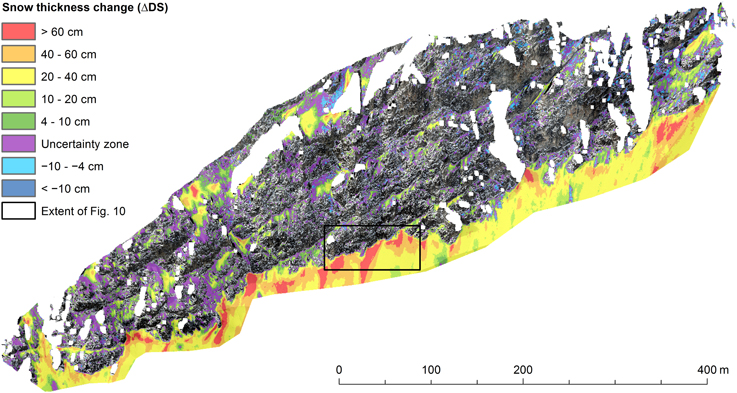
Figure 5. Spatial distribution of the snow accumulation during the snowfall. The area in the black rectangle is shown in detail in Figure 10. Most snow accumulated below the actual rock face. Within the rock face, ΔDS only reached high values locally. The spatial variability was high. The orientation of the rock face is similar to the view in Figure 1B.

The spatial patterns of the total snow thickness after the snowfall were similar to those of the snow thickness change (Figure 6). The correlation coefficient between DS and ΔDS is r = 0.86. The similarity also becomes evident by comparing Figures 5, 6. As an example, the areas with DS > 2 m correspond very well to the areas with ΔDS > 60 cm. This similarity indicates that the measured snowfall event is representative of most (larger) snowfalls during this winter. Similarly high correlations between the absolute snow thickness and snow accumulation were also found in gentler terrain by Schirmer et al. (2011) but only for snowfalls associated with a specific wind direction. Furthermore, the DS distributions of the different measurement days were also very similar. In fact, all correlation coefficients between these distributions are higher than 0.98. Consequently, only the distribution of 25 March is shown, where the spatial patterns are most evident. DS was highest in the “slope toe,” especially along the boundary to the actual rock face. There are several local maxima, where DS exceeded 4 m. This indicates that the observed avalanching took place everywhere in the rock face over the course of the winter, but that there were preferred avalanche tracks where avalanches were larger and/or more frequent. In the “snowfields,” DS was generally lower. Most values were between ten centimeters and one meter, whereas DS exceeded one meter in almost all cells in the “slope toe.” In the “steep/rough” areas finally, the majority of cells have DS < 0.1 m and there are many small negative values due to measurement noise (see also Figure 4C).

FIGURE 6

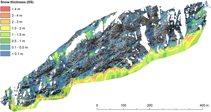
Figure 6. Spatial distribution of snow thickness on 25 March. Most snow lay at the top of the “slope toe.” The spatial patterns of DS were very similar to those of ΔDS. The orientation of the rock face is similar to the view in Figure 1B.

3.2. Redistribution of Snow After The Snowfall Event

We hypothesize that the snow redistribution, which started during the snowfall (Figure 5), continues for several days after the snowfall ceases and that snow is redistributed from extremely steep to flatter areas within the rock face. Figure 7 shows the evolution of snow covered area (SCA) in the rock face. SCA is the ratio between the snow-covered and the total surface area (Fierz et al., 2009). By definition of the subareas, the “slope toe” was almost completely snow-covered, whereas the “steep/rough” areas were mostly snow-free before the snowfall. On 25 March, however, almost 40% of this subarea was snow-covered. SCA strongly decreased in the “steep/rough” areas between 25 and 28 March, especially compared to the “snowfields.” After 28 March, the rate of decrease was similar in both subareas. This suggests that snow was redistributed from the “steep/rough” areas to the “snowfields” between 25 and 28 March. It is likely that the strong decrease of SCA in the “steep/rough” areas was also partly caused by melt. Results show that extremely steep terrain can accumulate some snow during a snowfall event but cannot retain all of it.

FIGURE 7

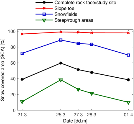
Figure 7. Evolution of snow covered area (SCA) in the rock face. After a marked increase during the snowfall, SCA reattains pre-snowfall values a week later. Note the strong decrease in the “steep/rough” areas compared to the “snowfields” between 25 and 28 March.

Figure 8 presents the evolution of the snow thickness relative to 21 March. The point measurements at the flat-field reference station Weissfluhjoch (WFJ) are shown in addition to the TLS results. DS increased in the “snowfields” between 25 and 27 March. This supports the hypothesis that snow is being redistributed from very steep to flatter areas. However, the data from the “steep/rough” areas do not support this. There, DS remained constant between 25 and 27 March and did not decrease. During the same period, small avalanches were observed to redistribute snow to the “slope toe.” Notwithstanding, DS decreased in this subarea. This could be explained by snow settling. Large amounts of fresh snow accumulated in the “slope toe” during the snowfall event (Figure 5). Loose snow settles quickly and this effect may have dominated the snow redistribution. There was less fresh snow in the “snowfields.” Hence, snow settling was less pronounced in this subarea. Between 25 and 27 March, the decrease of DS was 50% lower in the “slope toe” than at the reference station WFJ. The amount of fresh snow was only 10% lower. The difference can therefore not be attributed to settling alone. The decrease may have been lower in the “slope toe” because of the redistribution of snow. The decrease of DS at WFJ can be assumed to have been largely due to settling because there was practically no wind (see Section 2.3). There were some gusts that could have transported snow but only during short periods. After 27 March, the rate of decrease at WFJ and in the “slope toe” was similar. This supports the hypothesis that snow is redistributed only during the snowfall event (Section 3.1) and 2 or 3 days thereafter (provided that there is no strong wind).

FIGURE 8

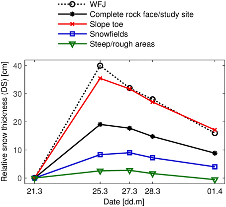
Figure 8. Evolution of the snow thickness relative to 21 March. WFJ: reference station at Weissfluhjoch. Note the increase in the “snowfields” between 25 and 27 March as well as the stronger decrease at WFJ compared to the “slope toe” in the same period.

3.3. Snow Accumulation at the Slope Toe Boundary

A recurring pattern of snow accumulation was observed at transitions from moderately steep to extremely steep terrain. The snow thickness change decreased rapidly across such boundaries (Figure 9). The boundary between the “slope toe” and the actual rock face is considered in this section (henceforth referred to as slope toe boundary or ST-boundary). The same pattern was also observed at the upper boundaries of snowfields, however. The averaged transects in Figure 9 were calculated as illustrated in Figure 10. The ST-boundary was shifted vertically in steps of 0.5 m (the raster size) and mean values were calculated along those lines. An averaged transect is much more representative than a single transect at an arbitrary location. The averaged transects were calculated in the area shown in Figure 10 because the ST-boundary was very clear in this area. The winter slope angle rises slowly in the upper part of the “slope toe” and then increases rapidly to over 70° across the ST-boundary. The summer slope angle is higher and less regular. This indicates that the snow-free surface is rougher than the snow surface (Mott et al., 2011; Schirmer et al., 2011). Below −15 m, winter and summer slope angles are nearly identical. More snow accumulated close to the ST-boundary than further down in the “slope toe.” The snow thickness change reached a maximum of 60 cm only several meters away from the ST-boundary. The value of the maximum is another indication of snow redistribution during the snowfall (Figure 5) because ΔDS at WFJ was only 40 cm (Figure 8). The snow thickness change decreased rapidly across the ST-boundary. However, a considerable amount of snow accumulated in very steep terrain. ΔDS remained above 50 cm in terrain up to 70° steep. If we consider the winter slope angle, which may be more relevant for the snow thickness change, ΔDS was higher than 50 cm in areas up to 50° steep. At 70°, the snow thickness change was still 20 cm.

FIGURE 9

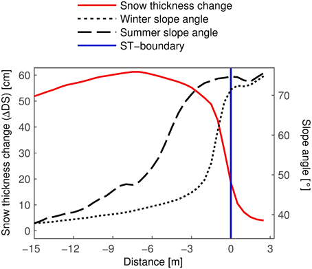
Figure 9. Averaged transects of ΔDS (between 21 and 25 March) and winter and summer slope angle. The x-axis gives the distance from the ST-boundary. Negative values lie in the “slope toe.” ΔDS attained a maximum at –7 m and then decreased rapidly closer to the ST-boundary.

FIGURE 10

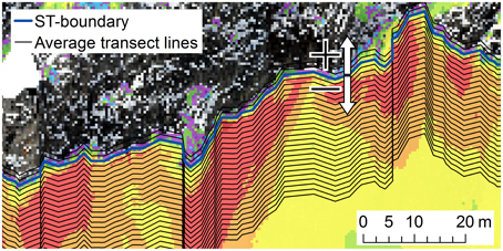
Figure 10. Illustration of how the average transects in Figures 9 and 11 were calculated. The mean values were calculated along the average transect lines. Only every second line is shown. The ST-boundary is defined by the snow cover extent of 21 March. The location of this detail is shown in Figure 5. The arrows show in which direction the distance is positive or negative.

The DS transects (Figure 11) were calculated the same way as the ΔDS transect (Figure 9). The DS and ΔDS transects have similar shapes. However, there appears to be a horizontal shift of about −3 m. ΔDS was maximal at around −7 m and began to decrease rapidly at −2 m. In the case of the DS transects these two distances were −10 and −5 m. Furthermore, the maxima in the DS transects were less pronounced. The horizontal shift could be explained by avalanching. Many small, loose-snow avalanches were observed by eye. Most of them released right below the ST-boundary and were only several meters long. The maximum of ΔDS may also be located differently for each snowfall event. This would also explain why the DS maxima were less pronounced. Snow creep (McClung, 1980; Abe, 2001; Teufelsbauer, 2011) is another process which transports snow downhill. However, creep velocities are of the order of one millimeter per hour (Exner and Jamieson, 2009). It would thus take about 4 months for the maximum to be shifted by 3 m. The total amount of snow at the slope toe boundary was considerable. On 25 March, DS was above 2 m in terrain up to 60° steep (summer slope angle). At 70°, there was more than one meter of snow. The very steep terrain considered here was able to hold most of the fresh snow for at least 10 days. Until 1 April, DS did not decrease much in terrain steeper than about 65°. In flatter terrain, on the other hand, the decrease between 25 March and 1 April was considerable. This may be due to snow settling (Section 3.2).

FIGURE 11

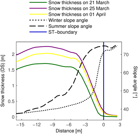
Figure 11. Averaged transects of snow thickness on different days and of winter and summer slope angle. DS did not decrease much in the extremely steep terrain. The curves are similar to the ΔDS transect (Figure 9) but with a horizontal shift of about −3 m.

3.4. Snow Accumulation in Very Steep Terrain

The averaged transects in Figures 9, 11 showed that the snow thickness and the snow thickness change both tended to zero in terrain steeper than 70°. It is important to note that these results are only valid in the area shown in Figure 10. In fact, the results are quite different when the complete rock face/study site is considered (Figure 12). This discrepancy reveals that the area considered for the transects is not representative of the complete area of interest. To plot the curves in Figure 12, the rock face was subdivided in (summer) slope angle classes of two degrees and mean values were computed for the snow thickness on 25 March and the snow thickness change during the snowfall. The class width of two degrees ensures that each class (above 30°) contains a minimum of more than 900 cells. The curves begin at 30° because there are practically no cells with a slope angle below that value. At first, DS and ΔDS decreased rapidly with increasing slope angle. At 50°, ΔDS began to flatten out and reached a value of about 10 cm, at which it remained up to 90°. DS leveled out starting at about 60° and stabilized at a value of about 0.25 m. An interesting feature in both graphs is the plateau between 35 and 40°. Almost the complete “slope toe” falls into this range of slope angles. Snow was accumulated more evenly in this gentler terrain, at least with respect to the slope angle. The high variability of ΔDS and DS (Figures 5, 6) appears to be related to other processes and parameters.

FIGURE 12

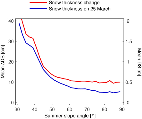
Figure 12. Mean snow thickness and snow thickness change in slope angle classes of 2°. The complete rock face/study site is considered. After a rapid decrease, the curves flatten out and remain constant up to 90°. Note the plateau between 35 and 40°.

The amount of snow in extremely steep terrain is considerable (Figure 13). To obtain the curves in Figure 13, the snow volume in each slope angle class was normalized by the respective number of cells. The cumulative sum of these normalized values was divided by the total normalized volume such that the curves reach 100% at 90°. In other words, Figure 13 presents the normalized integrals of the curves in Figure 12 (see also Appendix). The cumulative distributions became flatter between 40 and 50° and then increased uniformly to 100%, reflecting the almost constant values of ΔDS and DS at high slope angles (Figure 12). The shapes of the curves were similar but the distribution corresponding to the total amount of snow always had a higher value. The difference between the two curves is another indication of the redistribution of snow taking place after the snowfall. While areas steeper than 60° accumulated close to 18% of the snow during the snowfall event, the same areas “only” contained about 12% of the total amount of snow. This shows that the extremely steep terrain could not hold all of the snow that was deposited there during the snowfall event. Nevertheless, the amount of snow in near-vertical terrain is remarkably high.

FIGURE 13

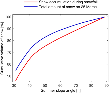
Figure 13. Cumulative distribution of the normalized snow volume as a function of the summer slope angle. Calculated for slope angle classes of 2°. The complete rock face/study site is considered. More than 10% of the total amount of snow lay in areas steeper than 60°.

4. Discussion

One of the aims was to develop a postprocessing procedure for TLS data specifically adapted to rock faces. The main innovations were the use of snow thickness instead of snow depth and the consistent application of MSA to improve the registration between the measurement days. Wirz et al. (2011) transformed the scanned surfaces to global coordinates (CH1903) and computed differences between them in this frame of reference. We calculated the snow thickness change in the MSA-corrected frame of reference and transformed them to global coordinates afterwards. The achieved precision (standard deviation < 5 cm) was similar to observations in gentle terrain (Grünewald et al., 2010; Revuelto et al., 2014a). The transformation to global coordinates relies on a usually very limited number of reflectors (≲ a dozen). MSA, on the other hand, uses up to hundreds of thousands of tie points. This leads to a much more robust and more precise registration. MSA can only be applied if the target surface includes enough stationary areas. These parts of the target must also be distinguishable from the non-stationary parts. A rock face usually fulfils these requirements, at least at a time scale of weeks. At a time scale of years, however, rockfall may substantially alter the appearance of a rock face.

Snow appears to be able to accumulate permanently at all slope angles. We observed constant values of DS and ΔDS at slope angles between ~70 and 90°. (Figure 12). Several authors have assumed that no snow can be retained in such terrain (Winstral et al., 2002; Gruber Schmid and Sardemann, 2003; Machguth et al., 2006). Our results suggest that the assumption of a positive constant may be more appropriate. This approach was in fact chosen by Bernhardt and Schulz (2010). They assumed an exponential decrease of the snow holding depth but set a constant value of 5 cm at slope angles above 75°. The value of the constant is expected to strongly depend on the micro-topography of the rock face. Haberkorn et al. (2015) suggest that rough, step-like topography is necessary for permanent snow accumulation in near-vertical terrain. They argue that snow and rime can only temporarily adhere to near-vertical, smooth rock. In such a case, the DS-constant would be zero but a positive constant could still be assumed for ΔDS. Lehning et al. (2011) and Wirz et al. (2011) observed that rougher terrain accumulates less snow than smoother areas. This result may be invalid in near-vertical terrain. The constant may also depend on climate and on the spatial resolution, i.e., the grid size of the ΔDS and slope angle rasters. Blöschl et al. (1991) suggest that “warm” snow (maritime climate) may accumulate more easily in extremely steep terrain than “cold” snow (continental climate) because the latter does not sinter as quickly and is thus more susceptible to redistribution. The grid size may have a large influence on results in near-vertical terrain. A high resolution is needed to detect small rock ledges which appear essential for snow accumulation in such terrain. Finally, the type of stone (chemical composition) may also affect the value of the constants.

The cumulative distributions presented in Figure 13 depend on how the extent of the rock face is defined. In fact, the extent should be chosen such that two conditions are fulfilled. First, the area of interest should encompass a closed system with regard to deposited snow, i.e., once deposited, no snow should cross the boundary of the area of interest (AI-boundary). Second, the area of interest should include a sufficient number of cells at every slope angle. Neither condition was completely fulfilled in this study. The first condition is always hard to satisfy due to drifting snow. In this study, it is also likely that avalanches crossed the AI-boundary in the slope toe. Because avalanches redistribute snow from steeper to flatter areas, this means that the cumulative distributions are likely to be higher in reality than shown in Figure 13. The second condition is easier to verify. In this case, the area of interest contained only 933 cells with slope angles below 30° and none with slope angles below 10°. Such flat areas are expected to contain a large amount of snow. Their inclusion in the area of interest would therefore lead to even higher values of the cumulative distributions. Thus, the values given for the relative amount of snow in extremely steep terrain may be lower if an area satisfying the two conditions were considered. However, as shown in the Appendix, the values would probably be only slightly smaller. It is estimated that areas steeper than 60° contained about 10% of the total amount of snow and accumulated almost 15% of the snow during the snowfall event. The measured values using the area of interest with an imperfect fulfillment of the conditions were 12 and 18%.

Avalanching seems to be the main process involved in the redistribution of snow, both during and after the snowfall. Many small avalanches were observed visually. The accumulation patterns in the “slope toe” do not resemble “normal” avalanche deposits, however. There are no sharp transitions in the snow thickness change. The Schiahorn rock face is so steep that avalanches do not slide but fall down. This leads to accumulations of loose snow with poorly defined borders. The falling snow accumulates at the top of the “slope toe” close to the actual rock face. This explains the maxima in the transects of DS and ΔDS. The relatively high correlations between the winter slope angle and ΔDS and between the summer slope angle and DS provide additional evidence of the importance of avalanching because this gravitational effect is also closely related to the slope angle. These observations are in contrast to the results of Wirz et al. (2011), where wind was identified as the main cause for the observed DS distribution. Whereas wind speeds were high during most snowfalls studied by Wirz et al. (2011), they were low during the snowfall event investigated here (Section 2.3). This may explain why our correlation coefficients between slope angle and DS (and ΔDS) were much higher than those of Wirz et al. (2011). It is also possible that the correlations were higher because the Schiahorn rock face is much steeper than the Chüpfenflue studied by Wirz et al. (2011). The importance of gravitational effects is expected to increase with the steepness of the terrain. In a rock face as steep as the Schiahorn, avalanching may even be the dominant process during snowfalls accompanied by wind. The observed changes in snow thickness cannot be attributed to snow redistribution alone. Warm temperatures and shortwave radiation may have caused some melt. This is especially likely in the “steep/rough” areas where the snow cover was thin and interspersed with snow-free rock areas.

Another process that may influence the distribution of ΔDS during snowfalls is preferential deposition. The effect of topography on the atmospheric flow field leads to an uneven deposition of snow at small scales. In particular, more snow accumulates on the leeward slope than on the windward slope of ridges (Lehning et al., 2008; Mott et al., 2014; Revuelto et al., 2014b). At the scale of a single slope, the ambient turbulence close to the surface may have an effect on the falling snow particles that would lead to preferential deposition of snow in less steep parts of the slope. The relevance of this effect is unknown and because preferential deposition and avalanching would affect the accumulation distribution similarly, it may be difficult to distinguish the two processes based on experiments only. Numerical simulations may shed some light (Bernhardt et al., 2010; Dadic et al., 2010; Mott and Lehning, 2010; Mott et al., 2010; Warscher et al., 2013).

5. Conclusions and Outlook

The quality of TLS data from rock faces strongly depends on the postprocessing. We propose to use snow thickness instead of snow depth and, if possible, to consistently apply MSA to improve the registration. Furthermore, the view direction should be adapted to the rock face under consideration. To further improve data quality, the spatial resolution of the point clouds should be increased. This can be achieved either by decreasing the distance between the rock face and the scan position or by using a TLS with a smaller beam divergence.

Snow in rock faces should not be neglected in hydrological models. Even though more snow accumulates in moderately steep terrain, the amount of snow in extremely steep areas is considerable. Terrain steeper than 60° contained an estimated 10% of the total amount of snow. The same areas accumulated 15% of the fresh snow during the observed snowfall. The fresh snow was partly redistributed, both during and after the snowfall. In our case, many small avalanches redistributed snow from the steeper to the flatter parts of the rock face.

Since the support area for this investigation was small and observations were from a single rock face with specific properties such as exposition, climate etc., the results should be generalized in the future by investigating additional rock faces with diverse characteristics and from a variety of climates. The processes of snow redistribution should be further investigated. Wind and avalanching were both observed to be important factors, but their relevance appears to strongly depend on the characteristics of the rock face and on the weather conditions during the snowfall. Furthermore, it remains unclear how much melt contributes to the observed snow thickness changes. An important step in the necessary generalization will be to try to distinguish and quantify processes that contribute to the observed snow relocation or melt. A development step in this direction could be to install a permanent scanning device, which automatically scans a rock face in regular (short) intervals such that gravity relocation (avalanches and slides) can be distinguished from melt or wind transport of snow. Modeling these processes is a complementary step and can in principle be tackled with a combination of very high resolution wind and snow transport models (Mott and Lehning, 2010; Groot Zwaaftink et al., 2014), simple parametrization of slides (Bernhardt and Schulz, 2010) and advanced energy balance melt modeling (Mott et al., 2015). However, model application to such extreme terrain has not been achieved to date and presents a major challenge for the future.

Author Contributions

CS did the research and wrote the manuscript. ML and RM conceived and supervised the project, provided guidance, helped with the field work and analysis and revised the manuscript.

Conflict of Interest Statement

The authors declare that the research was conducted in the absence of any commercial or financial relationships that could be construed as a potential conflict of interest.

The Associate Editor Olaf Eisen declares that, despite having collaborated with author Michael Lehning, the review process was handled objectively.

Acknowledgments

We would like to thank Thomas Grünewald and Robert Kenner for their introduction to terrestrial laser scanning and the postprocessing software, Sebastian Schlögl for his help during the field work and Sophia Haussener for the discussions and feedback.

References

Abe, O. (2001). Creep experiments and numerical simulations of very light artificial snow packs. Ann. Glaciol. 32, 39–43. doi: 10.3189/172756401781819201

CrossRef Full Text | Google Scholar

Anderton, S. P., White, S. M., and Alvera, B. (2002). Micro-scale spatial variability and the timing of snow melt runoff in a high mountain catchment. J. Hydrol. 268, 158–176. doi: 10.1016/S0022-1694(02)00179-8

CrossRef Full Text | Google Scholar

Bernhardt, M., Liston, G. E., Strasser, U., Zängl, G., and Schulz, K. (2010). High resolution modelling of snow transport in complex terrain using downscaled MM5 wind fields. Cryosphere 4, 99–113. doi: 10.5194/tc-4-99-2010

CrossRef Full Text | Google Scholar

Bernhardt, M., and Schulz, K. (2010). SnowSlide: a simple routine for calculating gravitational snow transport. Geophys. Res. Lett. 37:L11502. doi: 10.1029/2010gl043086

CrossRef Full Text | Google Scholar

Blöschl, G. (1999). Scaling issues in snow hydrology. Hydrol. Process. 13, 2149–2175. doi: 10.1002/(SICI)1099-1085(199910)13:14/15<2149::AID-HYP847>3.0.CO;2-8

CrossRef Full Text | Google Scholar

Blöschl, G., and Kirnbauer, R. (1992). An analysis of snow cover patterns in a small alpine catchment. Hydrol. Process. 6, 99–109. doi: 10.1002/hyp.3360060109

CrossRef Full Text | Google Scholar

Blöschl, G., Kirnbauer, R., and Gutknecht, D. (1991). Distributed snowmelt simulations in an alpine catchment: 1. Model evaluation on the basis of snow cover patterns. Water Resour. Res. 27, 3171–3179. doi: 10.1029/91WR02250

CrossRef Full Text | Google Scholar

Boehler, W., Bordas-Vicent, M., and Marbs, A. (2003). “Investigating laser scanner accuracy,” in Proceedings of the 19th CIPA Symposim, 30 Sep- 4 Oct 2003 (Antalya).

Google Scholar

Dadic, R., Mott, R., Lehning, M., and Burlando, P. (2010). Parameterization for wind-induced preferential deposition of snow. Hydrol. Process. 24, 1994–2006. doi: 10.1002/hyp.7776

CrossRef Full Text | Google Scholar

Deems, J. S., Fassnacht, S. R., and Elder, K. J. (2006). Fractal distribution of snow depth from lidar data. J. Hydrometeorol. 7, 285–297. doi: 10.1175/JHM487.1

CrossRef Full Text | Google Scholar

Deems, J. S., Painter, T. H., and Finnegan, D. C. (2013). Lidar measurement of snow depth: a review. J. Glaciol. 59, 467–479. doi: 10.3189/2013JoG12J154

CrossRef Full Text | Google Scholar

El khrachy, I. (2008). Towards an Automatic Registration for Terrestrial Laser Scanner Data. Ph.D. thesis, Technische Universität Carolo-Wilhelmina zu Braunschweig.

Exner, T., and Jamieson, B. (2009). “The effect of daytime warming on snowpack creep,” in International Snow Science Workshop. 27 September to 2 October 2009, Davos, Switzerland. Proceedings, eds J. Schweizer and van A. Herwijnen (Birmensdorf: Swiss Federal Institute for Forest; Snow and Landscape Research WSL), 271–275.

Google Scholar

Fierz, C., Armstrong, R., Durand, Y., Etchevers, P., Greene, E., McClung, D., et al. (2009). The International Classification for Seasonal Snow on the Ground. IHP-VII Technical Documents in Hydrology No 83, IACS Contribution No 1. UNESCO-IHP, Paris.

Groot Zwaaftink, C. D., Diebold, M., Horender, S., Overney, J., Lieberherr, G., Parlange, M. B., et al. (2014). Modelling small-scale drifting snow with a lagrangian stochastic model based on large-eddy simulations. Boundary Layer Meteorol. 153, 117–139. doi: 10.1007/s10546-014-9934-2

CrossRef Full Text | Google Scholar

Gruber, S., Hoelzle, M., and Haeberli, W. (2004). Rock-wall temperatures in the alps: modelling their topographic distribution and regional differences. Permafrost Periglacial Process. 15, 299–307. doi: 10.1002/ppp.501

CrossRef Full Text | Google Scholar

Gruber Schmid, U., and Sardemann, S. (2003). High-frequency avalanches: release area characteristics and run-out distances. Cold Reg. Sci. Technol. 37, 439–451. doi: 10.1016/S0165-232X(03)00083-1

CrossRef Full Text | Google Scholar

Grünewald, T., and Lehning, M. (2011). Altitudinal dependency of snow amounts in two small alpine catchments: can catchment-wide snow amounts be estimated via single snow or precipitation stations? Ann. Glaciol. 52, 153–158. doi: 10.3189/172756411797252248

PubMed Abstract | CrossRef Full Text | Google Scholar

Grünewald, T., Schirmer, M., Mott, R., and Lehning, M. (2010). Spatial and temporal variability of snow depth and ablation rates in a small mountain catchment. Cryosphere 4, 215–225. doi: 10.5194/tc-4-215-2010

CrossRef Full Text | Google Scholar

Haberkorn, A., Phillips, M., Kenner, R., Rhyner, H., Bavay, M., Galos, S. P., et al. (2015). Thermal regime of rock and its relation to snow cover in steep alpine rock walls: gemsstock, central swiss alps. Geogr. Ann. Ser. A Phys. Geogr. 97, 579–597. doi: 10.1111/geoa.12101

CrossRef Full Text | Google Scholar

Heritage, G. L., and Large, A. R. (eds.). (2009). Laser Scanning for the Environmental Sciences. Chichester: John Wiley & Sons Ltd.

Google Scholar

Kenner, R., Phillips, M., Danioth, C., Denier, C., Thee, P., and Zgraggen, A. (2011). Investigation of rock and ice loss in a recently deglaciated mountain rock wall using terrestrial laser scanning: gemsstock, swiss alps. Cold Reg. Sci. Technol. 67, 157–164. doi: 10.1016/j.coldregions.2011.04.006

CrossRef Full Text | Google Scholar

Lehning, M., Grünewald, T., and Schirmer, M. (2011). Mountain snow distribution governed by an altitudinal gradient and terrain roughness. Geophys. Res. Lett. 38:L19504. doi: 10.1029/2011gl048927

CrossRef Full Text | Google Scholar

Lehning, M., Löwe, H., Ryser, M., and Raderschall, N. (2008). Inhomogeneous precipitation distribution and snow transport in steep terrain. Water Resour. Res. 44:W07404. doi: 10.1029/2007WR006545

CrossRef Full Text | Google Scholar

Lehning, M., Völksch, I., Gustafsson, D., Nguyen, T. A., Stähli, M., Zappa, M., et al. (2006). ALPINE3D: a detailed model of mountain surface processes and its application to snow hydrology. Hydrol. Process. 20, 2111–2128. doi: 10.1002/hyp.6204

CrossRef Full Text | Google Scholar

Lichti, D. D., and Jamtsho, S. (2006). Angular resolution of terrestrial laser scanners. Photogramm. Rec. 21, 141–160. doi: 10.1111/j.1477-9730.2006.00367.x

CrossRef Full Text | Google Scholar

Luetschg, M., Lehning, M., and Haeberli, W. (2008). A sensitivity study of factors influencing warm/thin permafrost in the swiss alps. J. Glaciol. 54, 696–704. doi: 10.3189/002214308786570881

CrossRef Full Text | Google Scholar

Machguth, H., Paul, F., Hoelzle, M., and Haeberli, W. (2006). Distributed glacier mass-balance modelling as an important component of modern multi-level glacier monitoring. Ann. Glaciol. 43, 335–343. doi: 10.3189/172756406781812285

CrossRef Full Text | Google Scholar

McClung, D. M. (1980). Creep and Glide Processes in Mountain Snowpacks. NHRI Paper No. 6. National Hydrology Research Institute, Ottawa, ON.

Mott, R., Daniels, M., and Lehning, M. (2015). Atmospheric flow development and associated changes in turbulent sensible heat flux over a patchy mountain snow cover. J. Hydrometeorol. 16, 1315–1340. doi: 10.1175/JHM-D-14-0036.1

CrossRef Full Text | Google Scholar

Mott, R., and Lehning, M. (2010). Meteorological modeling of very high-resolution wind fields and snow deposition for mountains. J. Hydrometeorol. 11, 934–949. doi: 10.1175/2010JHM1216.1

CrossRef Full Text | Google Scholar

Mott, R., Schirmer, M., Bavay, M., Grünewald, T., and Lehning, M. (2010). Understanding snow-transport processes shaping the mountain snow-cover. Cryosphere 4, 545–559. doi: 10.5194/tc-4-545-2010

CrossRef Full Text | Google Scholar

Mott, R., Schirmer, M., and Lehning, M. (2011). Scaling properties of wind and snow depth distribution in an Alpine catchment. J. Geophys. Res. 116:D06106. doi: 10.1029/2010jd014886

CrossRef Full Text | Google Scholar

Mott, R., Scipión, D., Schneebeli, M., Dawes, N., Berne, A., and Lehning, M. (2014). Orographic effects on snow deposition patterns in mountainous terrain. J. Geophys. Res. 119, 1419–1439. doi: 10.1002/2013jd019880

CrossRef Full Text | Google Scholar

Prokop, A. (2008). Assessing the applicability of terrestrial laser scanning for spatial snow depth measurements. Cold Reg. Sci. Technol. 54, 155–163. doi: 10.1016/j.coldregions.2008.07.002

CrossRef Full Text | Google Scholar

Prokop, A., Schirmer, M., Rub, M., Lehning, M., and Stocker, M. (2008). A comparison of measurement methods: Terrestrial laser scanning, tachymetry and snow probing for the determination of the spatial snow-depth distribution on slopes. Ann. Glaciol. 49, 210–216. doi: 10.3189/172756408787814726

CrossRef Full Text | Google Scholar

Revuelto, J., López-Moreno, J., Azorin-Molina, C., Zabalza, J., Arguedas, G., and Vicente-Serrano, S. (2014a). Mapping the annual evolution of snow depth in a small catchment in the Pyrenees using the long-range terrestrial laser scanning. J. Maps 10, 379–393. doi: 10.1080/17445647.2013.869268

CrossRef Full Text | Google Scholar

Revuelto, J., López-Moreno, J. I., Azorin-Molina, C., and Vicente-Serrano, S. M. (2014b). Topographic control of snowpack distribution in a small catchment in the central Spanish Pyrenees: intra- and inter-annual persistence. Cryosphere 8, 1989–2006. doi: 10.5194/tc-8-1989-2014

CrossRef Full Text | Google Scholar

Schirmer, M., Wirz, V., Clifton, A., and Lehning, M. (2011). Persistence in intra-annual snow depth distribution: 1. Measurements and topographic control. Water Res. Res. 47:W09516. doi: 10.1029/2010WR009426

CrossRef Full Text | Google Scholar

Schweizer, J., Jamieson, J. B., and Schneebeli, M. (2003). Snow avalanche formation. Rev. Geophys. 41:1016. doi: 10.1029/2002rg000123

CrossRef Full Text | Google Scholar

Teufelsbauer, H. (2011). A two-dimensional snow creep model for alpine terrain. Nat. Hazards 56, 481–497. doi: 10.1007/s11069-010-9515-8

CrossRef Full Text | Google Scholar

Warscher, M., Strasser, U., Kraller, G., Marke, T., Franz, H., and Kunstmann, H. (2013). Performance of complex snow cover descriptions in a distributed hydrological model system: a case study for the high alpine terrain of the berchtesgaden alps. Water Resour. Res. 49, 2619–2637. doi: 10.1002/wrcr.20219

PubMed Abstract | CrossRef Full Text | Google Scholar

Winstral, A., Elder, K., and Davis, R. E. (2002). Spatial snow modeling of wind-redistributed snow using terrain-based parameters. J. Hydrometeorol. 3, 524–538. doi: 10.1175/1525-7541(2002)003<0524:SSMOWR>2.0.CO;2

CrossRef Full Text | Google Scholar

Wirz, V., Schirmer, M., Gruber, S., and Lehning, M. (2011). Spatio-temporal measurements and analysis of snow depth in a rock face. Cryosphere 5, 893–905. doi: 10.5194/tc-5-893-2011

CrossRef Full Text | Google Scholar

Witmer, U. (1984). Eine Methode Zur Flächendeckenden Kartierung von Schneehöhen Unter Berücksichtigung von Reliefbedingten Einflüssen. Bern: Band 21 von Geographica Bernensia; Geographisches Institut der Universität Bern.

Appendix

To estimate the cumulative distributions in an area satisfying the two conditions described in Section 4, we assume that the values measured at the lower AI-boundary in the slope toe change linearly to reach flat field values a certain distance away (see Figure A1). The values from the reference station WFJ are taken as the flat field values (DS = 1.68 m and ΔDS = 40 cm). The values at the lower AI-boundary are averages along this line (DS = 1.28 m and ΔDS = 31.7 cm). The summer slope angle at the lower AI-boundary is 36.3°.

FIGURE A1

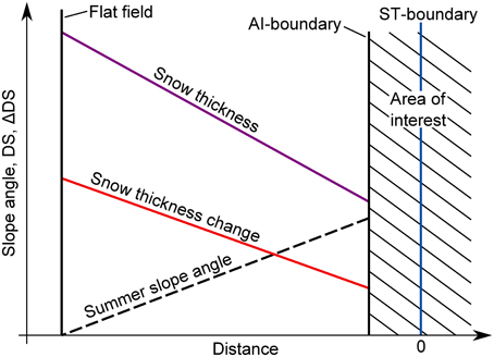
Figure A1. Estimation of the cumulative distribution of the normalized snow volume in an area encompassing all slope angles. A linear change of the variables is assumed between the AI-boundary in the slope toe and the virtual flat field conditions a certain distance away. The x-axis is the same as in Figures 9, 11.

The normalized volume of snow Ṽ in a certain subarea is the snow volume V divided by the number of cells N in this subarea. It can therefore be written as

$\begin{array}{l}Ṽ=\frac{V}{N}=\frac{\overline{\text{DS}}A}{N}=\overline{\text{DS}}{A}_c\end{array}$

where $\overline{\text{DS}}$ is the average snow thickness in this subarea, A is the surface area, and A_c is the surface area of a single cell. Relative amounts of snow, which are fractions of normalized snow volumes, are thus entirely defined by the average snow thicknesses in the considered subareas if the cell size is constant. In particular, they do not depend on the assumed distance between the lower AI-boundary and the virtual flat field. The distance can therefore be chosen, such that no avalanches cross the extended AI-boundary. With the exception of drifting snow, the condition of a closed system is thus fulfilled. The second condition, that the area contains areas of all slope angles is also fulfilled.

Because the variables are assumed to vary linearly, DS can easily be calculated for each slope angle class between 0° and 36°. The original area of interest contains slope angles between 10° and 90°. To calculate the overall cumulative distribution, we used the estimated values in the range 0° to 10°, the average of the estimate and the measurement between 10° and 36° and the measured values above 36°. This leads to the relative amount of snow in terrain steeper than 60° of 10%. The calculations are the same for the snow accumulation and result in a relative amount of 15%.