Metric-Resolution 2D River Modeling at the Macroscale: Computational Methods and Applications in a Braided River

Introduction

Digital terrain models (DTMs) describing the land surface of the earth are a critical resource for hydrologic studies, enabling a wide range of analyses of flow and transport phenomena. The spatial extent of DTMs varies from local to global scales, the resolution varies from centimeters to kilometers, and accuracies range from millimeters to tens of meters (Maune, 2001; Li et al., 2005; Yan et al., 2015a). For any particular DTM, the spatial extent, resolution, and accuracy will depend on the method of acquisition (e.g., terrestrial, aerial, satellite), the measurement sensor (e.g., lidar, photogrammetry, interferometry) and land cover (Maune, 2001; Li et al., 2005; Yan et al., 2015a). Additionally, DTMs may be produced from several data sources. For example, the National Elevation Dataset (NED) available in the United States merges the best available elevation data in different areas (Gesch et al., 2014), and DTMs of rivers and coastal waters, such as NOAA NGDC's integrated models of coastal relief (Eakins and Taylor, 2010), typically merge topographic and bathymetric data collected with different types of sensors. There has also been growing interest in developing lidar sensors capable of measuring both subaerial and subaqueous topography within the same flight pass (Fernandez-Diaz et al., 2014).

The practice of river modeling has been transformed by the proliferation of DTMs. Historically, hydraulic river models were supported by cross-sectional surveys of the channel geometry at a set of river transects, from which integral properties of the river needed for one-dimensional hydraulic analysis, such as the cross-sectional area and wetted perimeter, could be tabulated as a function of river stage (Cunge et al., 1980). But today, it is more common to access a river DTM than cross-sectional data, and popular one-dimensional modeling software such as HEC-RAS (US Army Corps of Engineers, Davis, California) is configured to compute transect data from DEMs using tools such as HEC GeoRAS (US Army Corps of Engineers, Davis, California). The increased availability of river DEMs has also enabled multi-dimensional hydrodynamic river modeling (both 2D and 3D) for numerous applications including studies of morphodynamics (Lane et al., 1999; Abu-Aly et al., 2014), ecology (Crowder and Diplas, 2000; Shen and Diplas, 2008), and flood risk (Sanders, 2007; Bates, 2012; Yan et al., 2015a). Indeed, multi-dimensional hydrodynamic river models offer exciting new opportunities to examine the complexity of river dynamics at fine scale and over spatial extents of practical significance (Wyrick et al., 2014). However, the computational demands of fine-resolution modeling are high which motivates research not only into more efficient numerical solution methods but also pre- and post-processing strategies because of large data volumes.

The primary factors affecting the computational demands of hydrodynamic river models are the number of computational cells and time steps required to span the domain and period of interest; computational costs generally scale as the product of these two factors (Kim et al., 2014). For example, a 100 km river reach with a 2 km wide floodplain is spanned by ~2.0 × 10⁸ metric resolution cells. Furthermore, 1.3 × 10⁷ time steps are needed to advance the solution for a period of a month based on a time step of 0.2 s which is typical of explicit flow models constrained by the Courant, Friedrichs, Lewy (CFL) for stability. Assuming about 100 floating point operations per cell per time step, the total operation count becomes 2.6 × 10¹⁷/simulation-month which calls for petascale computing power (10¹⁵ floating point operations per second). Memory demands for a domain of this size are roughly 30 GB assuming 20 double precision (8 byte) arrays, which is within the capabilities of typical high performance computing nodes (ca. 256 GB) but may exceed the capacity of a typical desktop computer at the present time.

High computational costs have generally limited the application of metric resolution models to the mesoscale defined by small multiples of the river width (e.g., Crowder and Diplas, 2000), although there have been a few applications at the macroscale defined by large multiples of the river width (e.g., Abu-Aly et al., 2014; Yan et al., 2015b). Macroscale hydrodynamic modeling is also somewhat common with a grid resolution of tens, hundreds or even thousands of meters, sometimes using sub-grid models to account for channel flows (e.g., Neal et al., 2012). Coarsening grid resolution makes hydrodynamic modeling far less demanding because with every doubling of the cell size, run times are reduced by a factor of eight (Kim et al., 2014). Macroscale models may also use a downscaling technique to create the appearance of metric-resolution hydrodynamic modeling after flow calculations are made on a much coarser grid (e.g., Schumann et al., 2014).

Dottori et al. (2013) caution that the cost of fine-resolution analysis may not be justified for flood inundation modeling, where the main goal is to predict flood stage and flood extent, given other sources of uncertainty. However, a number of researchers have found that a metric resolution is needed to reasonably approximate hydraulic habitat, i.e., local depth and velocity, which is relevant to river ecology and morphology (Crowder and Diplas, 2000; Cook and Merwade, 2009; Clifford et al., 2010; Williams et al., 2013; Abu-Aly et al., 2014). Furthermore, with the aid of analytical models for the vertical velocity distribution including a characterization of bed roughness, metric-resolution 2D models can reconstruct a 3D characterization of flow for a wide range of applications at far less computational expense than 3D models based on the Navier-Stokes equations (Begnudelli et al., 2010; Abu-Aly et al., 2014; Wyrick et al., 2014), although there are many examples of 3D flow phenomena that demand 3D models for an accurate description such as horseshoe vortices around bridge piers and similarly complex turbulent velocity fluctuations occurring around boulders, large bed forms, and other types of flow obstructions (Wu, 2007; Javernick et al., 2015).

Unstructured grids based on triangles can reduce the computational demand of 2D hydrodynamic models by localizing fine-resolution cells in selected areas, and allowing use a relative coarse (and less costly) cells in other areas. Triangular grids are also referred to as having a Triangular Irregular Network (TIN) data structure (Peucker et al., 1976; Tsai, 1993). Rivers with complex channel networks, islands, and tiered floodplains tend to be good candidates for triangular grids, while systems with relatively simple topography such as engineered channels with regular channel cross-sections are better suited to grids based on quadrilateral cells (Kim et al., 2014). Urban floodplains can present considerable topographic complexity in the form of narrow channels, flood walls, and building walls that affect the movement of flood water, and here triangular grids have proven to be excellent for 2D hydrodynamic modeling (Schubert et al., 2008; Gallegos et al., 2009; Sanders et al., 2010; Gallien et al., 2011; Schubert and Sanders, 2012; Costabile and Macchione, 2015). Although there are many grid generation tools available, a popular option for triangular grids is Triangle (Shewchuk, 1996), which allows the user to specify constraints on the position of grid vertices and the size of triangles. These features have enabled researchers to systematically use vector data archived in Geographic Information Systems (GIS) to constrain grids generated by Triangle, for example vector data describing building walls (Schubert et al., 2008), roads (Schubert and Sanders, 2012), sea walls (Gallien et al., 2011), channel banks (Kim et al., 2014), and bridge footings (Costabile and Macchione, 2015). These constraints are important not only to vary the spatial resolution of the grid, but also to accurately model channel shape and overtopping thresholds with a relatively coarse (and efficient) computational grid. Databases of linear features (e.g., US National Hydrologic Database) are seldom or not easily accessible and often lack sufficient detail and accuracy for metric resolution hydrodynamic modeling. For example, available data may be limited to an estimated channel centerline, and the location of the centerline is often displaced by tens of meters or more from the true centerline.

Hydrodynamic model grids need to resolve low flows, high flows, and the transition between these states. In meandering rivers with a single channel and relatively flat floodplain, accurate low flow modeling focuses attention on the thalweg and banks of channels and typically dictates the finest resolution adopted by an unstructured grid. Higher flood stages, on the other hand, are typically less demanding (Kim et al., 2014). Braided rivers (BR) are even more demanding to efficiently model because of the range of channel sizes, channel anastomosis, and extensive wetting and drying. A manual or semi-automated approach can be used at the mesoscale to delineate break lines to constrain unstructured mesh generation (Schubert et al., 2008; Gallegos et al., 2009; Gallien et al., 2011; Schubert and Sanders, 2012), but this becomes impractical at the macroscale. Macroscale applications of metric resolution models demand a fully automated grid generation technique.

The objectives of this paper are three-fold: (1) to present an automated method of unstructured grid generation to support efficient metric resolution hydrodynamic modeling of a BR, (2) to measure how application of BR model output for analyzing hydraulic geometry (HG) and hydraulic habitat is affected by grid resolution and resistance parameters, and (3) to demonstrate the application of a metric-resolution model at the macroscale including the necessary tools for pre- and post-processing and parallel computing. Furthermore, this study illuminates the richness of information about BRs that can be gleaned when the descriptive power of fine resolution mechanistic models is harvested at the macroscale. A broader goal of this paper is to motivate more research that addresses the computational efficiency of metric-resolution river modeling, including pre-processing and post-processing, to make the power of fine resolution mechanistic models more accessible to decision-makers charged with managing riverine systems.

The remainder of the paper is organized as follows: Section Materials and Methods presents a site description (Site Description and Available Data), model pre-processing steps to create the computational grid and set up the hydrodynamic model (Pre-processing), parallel computing methods to advance the solution (Flow Simulation), post-processing techniques to streamline analysis of model output (Post-processing), hydraulic geometry analysis (Hydraulic Geometry Analysis), and hydraulic habitat analysis (Hydraulic Habitat Analysis). Section Results and Discussion presents hydrology analysis at the mesoscale (Mesoscale Flow Modeling) and macroscale (Macroscale Flow Modeling), analysis of hydraulic geometry (Hydraulic Geometry), and analysis of hydraulic habitat (Hydraulic Habitat Classification), followed by Conclusions (Section Conclusion).

Materials and Methods

Site Description and Available Data

The study site is a 140 km reach of the central Platte River in Nebraska, USA, and is shown in Figure 1. The Platte River is located in the northern plain region of the United States and extends 500 km from the location of confluence of the North and South Platte Rivers in western Nebraska to the Missouri River along the eastern border of Nebraska. The river basin is characterized by a broad floodplain, which in its lower reaches is bordered by bluffs, and a wide and shallow sand-bedded BR. Figure 1 shows a section of the central Platte between the cities of Overton, NE and Chapman, NE. In this area the Platte River has a complex braided channel system with variable widths (see inset in Figure 2), the main thread varies from 50–100 m during low flows but expands to around 1 km during high flows, while small channels can be as narrow as 10 m. The longitudinal slope of the river is ~140 cm/km and bed material consists of gravels mixed with silts and sands (Condon, 2005). The Central Platte is an internationally significant habitat for migratory birds, including three species listed as endangered or threatened, and represents a critical stopover point on the North American Flyway (Kinzel et al., 2006). Habitat is threatened by regulatory controls on discharge for agricultural production, which have limited the exceedance of bankfull discharge that would otherwise disturb island sediments and limit the seeding of vegetation (Kinzel et al., 2006). The central and lower reaches of the Platte have demonstrated sensitivity to flooding with more than 12 flood events recorded since the year 2000. Flooding is generally triggered by heavy and prolonged rainfall events from storm systems passing through the area, and also by the addition of snow melt during the spring months.

FIGURE 1

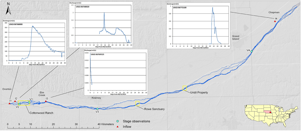
Figure 1. Overview of the modeled 140 km reach of the river Platte, with recorded discharge at four gages used for model forcing.

FIGURE 2

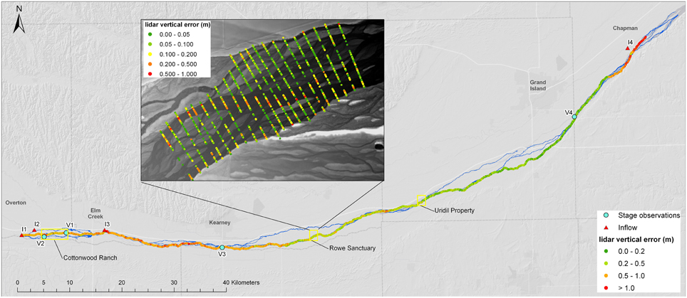
Figure 2. Lidar vertical error when compared to: thalweg data obtained from depth sounder (large image), RTK-GPS transects (inset). Inset also shows the complexity of river bathymetry at Rowe Sanctuary.

The Central Platte is the focus of the Platte River Recovery Implementation Program (PRRIP) which is an endangered species recovery and habitat restoration project supported by the States of Colorado, Nebraska, and Wyoming, the U.S. Department of the Interior, environmental groups, and local water users. Extensive data resources are available as a consequence of this project including aerial lidar data, channel bathymetry data, and stream gaging data.

A 1 m resolution 170 km DTM of the river corridor was available from topographic data collected using airborne light detection and ranging (lidar) flown in March 2009. The vertical accuracy of the DTM is better than 18 cm RMSE in open terrain (Dewberry, 2010). To validate the vertical accuracy of the DTM within the river channel, two datasets are available. The first consists of a thalweg vertical profile of the main river channel measured in April and August 2009 using a boat-mounted depth sounder in combination with real-time kinematic GPS (RTK-GPS). The vertical accuracy of the system is 3 cm root mean square error (RMSE; Ayers Associates and Olsson Associates, 2009). The second dataset consists of 78 transects of the main river channel within three properties along the river, Cottonwood Ranch, Rowe Sanctuary and the Uridil Property (see Figure 1). These properties are habitats designated to the protection of endangered and threatened species and are routinely monitored to study the effects of vegetation management on sediment transport and river morphology (Kinzel, 2008). The transects were measured during river low-flow in June 2008 using RTK-GPS with vertical accuracy better than 2 cm RMSE (Kinzel, 2008).

The overall vertical accuracy of the main channel thalweg, as captured by the lidar, is 0.65 m RMSE when compared to the sounder data. This accuracy varies substantially by sub-reach; the most upstream 53 km have a vertical RMSE of 0.82 m, the central 75 km an RMSE of 0.39 m and the most downstream 12 km an RMSE of 1.03 m (see Figure 2). These discrepancies are mainly attributable to differences in the river geomorphology: the top and bottom reaches have a narrower main channel (60–150 m) compared to the middle reach (90–270 m) resulting in increased flow depth. Since the lidar is unable to measure the submerged channel bathymetry at larger depths this results in an increased vertical error. Comparing lidar elevations with river transects at the three managed sites, Cottonwood Ranch, Rowe Sanctuary and Uridil Property, reveals accuracies of 0.25 m, 0.17 m, and 0.26 m RMSE, respectively. The inset in Figure 2 shows that the majority of each transect reports vertical errors < 10 cm, however these errors increase substantially toward the thalweg. Bearing in mind that the approximate depth of the main channel is 1.5 m, vertical errors in the deepest parts of the stream can amount to 30% of the channel depth. A small part of the vertical error may also be attributable to temporal decorrelation resulting from the dynamic nature of BR morphology, the transects were surveyed in June 2008 while lidar was flown in March 2009, however no major flow events were recorded within that time frame. The transects indicate that vertical errors for shallow braids are likely within the accuracy limitations of the lidar system, therefore suggesting that model results may be more accurate in shallow flow regions.

A month-long period, starting mid September 2013, was chosen for hydrodynamic modeling. The period corresponds to the rise and fall of a large flood, which occurred as a result of intense seasonal rainfall. The event was captured by several United States Geological Survey (USGS) stream gauges present within the 140 km reach. Table 1 summarizes the available gages within the modeling domain and describes their function for this study, while Figure S1 shows the hydrograph and resulting water levels at gauge I1. The models were initialized by low flows that were specified at the upstream boundary and progressively flooded the length of the model domain over the first week of the month long simulation period, so analysis of model data focuses on the final 3 weeks during which time flow transitioned from a low flow state of ~4 m³/s to a peak flow of over 300 m³/s and then back to a sustained flow ~80 m³/s by mid October 2013 (Figure S1). Figure S2 shows the cumulative distribution function at gage I1, which is used to force the model upstream boundary, as well as the minimum and maximum flows during the September 2013 flood event. Most flows considered during the event fall between the 5th and 90th percentile, which from a morphological perspective are important for minor channel adjustments and habitat but are not expected to cause major changes to the channel network or floodplain over the time scale.

TABLE 1

Table 1. Summary of gauges present in the modeled 140 km Platte river reach.

Figure 1 shows the location of gage I1, as well as other available gauges within the modeled reach. Table 1 provides an overview of how the gauges are used for modeling and validation. Gauges I2, I3, and I4 provide lateral inflows during the simulated period while gauges V1, V2, V3, and V4 are used for model validation. The hydrographs for the inflow gages are shown in Figure 1.

Metric-resolution river modeling at the mesoscale and macroscale is approached in three steps: pre-processing to transform a raster DTM into a unstructured mesh of triangular cells with minimal loss of flow-relevant topographic information, flow simulation with parallel computing, and post-processing to convert model output into a gridded form suitable for applications.

Pre-processing

Triangle constrained Delaunay grid generation software has been applied in numerous studies with breakline constraints to selectively refine unstructured grids and constrain the position of grid vertices to sample key topographic features (Schubert et al., 2008; Gallegos et al., 2009; Gallien et al., 2011; Schubert and Sanders, 2012). However, use of breaklines is not a good fit for BRs because of the channel network complexity which impedes manual delineation. Consequently, Triangle (Shewchuk, 1996) is applied here using point constraints which can be identified in an automated way. Point constraints were identified by processing the 1 m DEM using ArcGIS (ESRI, Redlands, California) for Very Important Points (VIPs) as follows: First, the standard deviation of DTM values in a 3 × 3 window surrounding each cell was computed and assigned to each 1 m resolution cell of a raster grid, then a threshold was introduced to retain only the largest values, or VIPs. The VIPs mark curvature in the DEM and generally correspond to channel banks. Next, a binary DTM was generated with a value of unity for any cell that contains a VIP, and a value of zero otherwise. The centroid coordinates of all cells containing VIPs were then input into Triangle along with a 30° angle constraint and the domain boundary to generate the computational grid. The process is akin to TIN generation whereby in this case greater effort is placed upon the representation of hydrologic features, rather than optimization to attain the best global representation of the surface within a set tolerance (Lee, 1991). As such it is more similar to a hydrographic TIN as described by Vivoni et al. (2004).

Triangle was applied to create mesoscale grids with resolutions of 5, 10, and 20 m (edge length) in areas with VIPs, and comparatively coarser, irregular cells in areas without VIPs such as channel bottoms, ponds and plateaus as shown in Figure S3C. Triangle was also applied to create a 5 m resolution mesoscale grid constrained by breaklines that were created by manually tracing channel bank visible when hillshade plots of the DEM were viewed in ArcGIS (ESRI, Redlands, California); this enables a comparison between breakline- and point-constrained grids. All mesoscale grids span the upper 14 km of the Platte River domain shown in Figure 1. Lastly, Triangle was applied to create a 5 m resolution macroscale grid that spans the entire 140 km domain shown in Figure 1 and consists of ~4.9 × 10⁶ vertices and 9.7 × 10⁶ computational cells. For all grids, elevations were assigned to each grid vertex (node) by nearest neighbor interpolation from the 1 m DEM.

Table 2 presents a summary of grids used in this study. Grids 1–3 correspond to macroscale domains, while Grids 4–7 correspond to mesoscale domains. Grid 1 represents the original lidar DTM at 1 m resolution used for comparison. Grid 2 is a 5 m re-sampled version of the original DTM while Grid 3 represents a VIP-constrained unstructured grid. Grid 4 is a 5 m resolution mesoscale grid constrained by breaklines, while Grids 5, 6, and 7 are 5, 10, and 20 m mesoscale grids constrained by VIPs, respectively.

TABLE 2

Table 2. Evaluation of mesh vertical accuracy based on 1000 randomly distributed points.

Table 2 shows that the number of cells in the macroscale unstructured grid (Grid 3) is 30 times smaller than in the original 1 m DTM (Grid 1), and it contains ~2 million fewer cells than the coarsened 5 m DTM (Grid 2). The unstructured grid represents a 20% reduction in the number of cells compared to the 5 m DTM, which may appear to be only a small advantage, but this difference was found to be important for two reasons. First, the unstructured grid clusters more computational resources in channels, and thus offers a better representation of channel flows below bank-full conditions. Secondly, further increases in the number of cells (in the 20% range) beyond the size of the unstructured grid pushed the limit of the desktop computing systems in use for pre-processing and post-processing, so the final unstructured mesh represented a limit for streamlined workflows on desktop computers. In terms of vertical accuracy, the errors of the unstructured grid are similar to the coarsened DTM, globally and within the channels, and remains well within the measurement uncertainty of the original lidar data. Figure S3 presents topographic shade plots of Grid 3 topographic features (Figure S3B) which compare favorably with the DTM (Figure S3A).

Table 2 also compares the mesoscale grids. The 5 m resolution VIP-constrained grid (Grid 5) contains approximately the same number of cells as the breakline-constrained grid (Grid 4), inside channels Grids 4 and 5 offer approximately the same vertical accuracy, and Grid 5 shows better accuracy across the floodplain. However, these differences are small, well within the bounds of measurement uncertainty, and therefore not viewed as significant. This indicates that the main advantage of using VIPs over breaklines for constraining Triangle grids is the capacity for automated grid generation. For Grid 6 and 7 corresponding to 10 and 20 m resolutions, respectively, vertical accuracies larger than the lidar vertical error are reported especially inside the channel. This suggests that grid coarsening beyond 5 m linear resolution may not yield accurate flow predictions.

Flow resistance in BRs is mainly related to sediment characteristics, and sediments are spatially variable as a result of ongoing sorting (Leopold and Wolman, 1957). The USGS and several private partners perform bed-sediment grain size analysis for the Platte River on a decadal basis, with the most recent survey occurring in 2009 (Kinzel and Runge, 2010). This data was not adequate for specifying the spatial distribution of sediment sizes (and thus a distribution of the Manning resistance parameter) between river bed and floodplain. Furthermore, a temporally coinciding spatial classification of landcover for the modeling domain was not available at sufficient resolution to accurately derive floodplain surface resistance, especially for a system as morphologically active as the Platte River. Consequently, each grid was parameterized with a spatially uniform Manning n = 0.028 m^−1∕3 s. This value was determined by first computing the median grain size of sediment in the study area, based on the average of data in the Overton-Grand Island reach, and then using look-up tables to arrive at a Manning coefficient value (Acrement and Schneider, 1984). Additionally, to measure the sensitivity of model output to the resistance parameter, a mesoscale model (Grid 6) was set up to use one of three different spatially uniform Manning coefficients, n = 0.025 m^−1∕3 s, 0.028 m^−1∕3 s, and 0.035 m^−1∕3 s.

Flow Simulation

The shallow-water equations are solved using a Godunov-type finite volume scheme, ParBreZo, that has been designed for applications with complex topography, mobile wet/dry fronts, hydraulic jumps, and any combination of sub-critical and super-critical flow (Kim et al., 2014). The flow solver is first-order accurate in time and space, but it takes advantage of a second-order accurate depiction of topography (the TIN is a piecewise linear topographic model) to achieve an effective convergence rate between first and second order, which is attributed to the dominant role of topographic uncertainty in flow prediction errors (Begnudelli et al., 2008). Other features of the algorithm include the use of a local time stepping scheme (Sanders, 2008), semi-implicit treatment of friction terms so frictional effects never constrain the time step (Begnudelli and Sanders, 2007), and the flexibility to use a combination of triangular and quadrilateral cells (Kim et al., 2014).

ParBreZo uses the Single Process Multiple Data (SPMD) approach for parallel execution on either shared-memory or distributed-memory multi-core computing systems and speedup has been shown to be linear with processors as desired with parallel computing (Sanders et al., 2010). ParBreZo was implemented on a single 64-core node with 2.33 GHz computing cores and 512 GB of fast 1600 MHz RAM. The macroscale model (Grid 3) was divided into 64 sub-grids and run on all 64 cores. The Metis graph partitioning library (Karypis and Kumar, 1999) was used for domain decomposition as described by Sanders et al. (2010). On the other hand, the mesoscale models were run on a single grid using 16 cores due to the modest computational costs and memory requirements. Computational effort is greater for wetted cells vs. dry cells, and this can lead to an imbalanced computational load among subdomains with equal numbers of cells (Sanders et al., 2010). No attempt was made to balance the load in this case because the areas of flooding evolve over time with the flood and the model is not designed for dynamic adjustments of the domain decomposition.

The 30 day simulation period was integrated on all grids with a variable time step that maintained a maximum Courant number of 0.8. During each run, the time step decreased from deciseconds to centiseconds with the rising flood stage, and increased again as the flood receded. The solution was saved daily in an ASCII text file. Cell center data was interpolated at vertices of the TIN (from cell centers) and exported as unstructured point data. Variables output included the free surface elevation, storage, and two components of velocity.

A full calibration of the meso-and macro-scale models was not attempted for several reasons. First, it has been recognized that height and velocity data to constrain spatially distributed flow models are generally quite limited (Schumann et al., 2009), as is the case here. Available data for calibration/validation are limited to two and four points within the mesoscale and macroscale models respectively, while the model domains consist of hundreds of thousands of cells (unknowns) at the mesoscale and millions of cells at the macroscale. The data are especially sparse considering that BRs exhibit a high degree of spatial variability in stage due to shallow depths and relatively large morphological features (e.g., Figure 7 shows bank to bank variability in stage height exceeding 1 m). The implication is that stage measurements only inform model predictions for a short distance around the gage. Secondly, as a result of shallow depths and large bedforms, calibration would demand simultaneous consideration of topographic data and resistance parameters (e.g., Yan et al., 2015b), and here both are spatially distributed fields leading to a massive number of unknown parameters. In applications that are supported by a spatial classification of land cover (e.g., Schubert et al., 2008; Abu-Aly et al., 2014), the number of calibration parameters can be reduced to the number of landcover classes but such information was not available at this site at an adequate resolution to discern between features such as channels and islands, and even if it were, the issue of calibrating uncertain topography remains. Third, models require lengthy computation times. For the macroscale model at 5 m resolution execution required 30 days of wall-clock time, using 64 processing cores, to simulate the 30 day high flow event. The mesoscale run times, using 16 processors, varied from a few hours up to 5 days depending on resolution. These run times made it prohibitive to apply an iterative process of adjusting model parameters to minimize the difference between model predictions and flow observations.

The lack of formal calibration is not a barrier in this study because the main objective is to present a method of automated mesh generation that can be used to develop efficient unstructured meshes of a BR, and because we have objectively measured the accuracy of meshes with respect to topography as described above (see Section Pre-processing). Hence, we adopt the 5 m model as a base-case because this yields the smallest errors in topographic heights, and because of a priori knowledge of the strong link between topographic data and flow predictions in BRs. The base case also uses a spatially uniform Manning resistance parameter representative of the median grain size (0.028 m^−1∕3 s). Furthermore, mesoscale models at 10 m and 20 m resolution are run to measure differences in model predictions attributable to mesh coarsening, and we measure differences in model predictions attributable to uncertain resistance parameters with an additional set of model runs. This yields a first order approximation of flow prediction uncertainties.

Another uncertainty not considered in the modeling process is due to stream morphodynamics. Although geomorphic changes due to large flow events are likely to occur in any soft bottom river channel, BRs are especially subjected to change due to the shallow nature of the individual braids, and the many instream features such as sandbars and islands (10⁰–10¹⁰ m scale). Due to the modeled event being of moderate proportion (average exceedance probability 26%) we do not expect island and floodplain morphology to be affected beyond the finest model resolution (5 m). However, channel banks and features such as sandbars (10⁰–10¹ m scale) could be affected by the flow. Previous research has shown that sandbars in BRs with similar characteristics to the Platte can migrate by 1–30 m over the course of 1 year (Sanford, 2007).

Since the model predictions are not calibrated and validated, the decision-support potential of the model is limited. That is, confidence in model predictions is not as high as one could expect from a calibrated model. Furthermore, since morphological processes are not considered, applications of the methodology to large flow events is not recommended. These issues could be very important to managers of riverine systems who use hydrodynamic models to inform maintenance, operations, and restoration programs, although reported uncertainties in model predictions may also be valuable for decision-support.

Post-processing

Unstructured point data from the model were converted into a raster format to facilitate applications of the model data (Wyrick et al., 2014), namely the potential to easily image the data and operate on it with image-based algorithms. This constitutes an interpolation problem, and standard routines in ArcGIS (ESRI, Redlands, California) were found to demand hours of computing time for this task because of the large number of data points (mesh vertices). For each interpolation point, a search of all data points is completed to find the nearest neighbors, resulting in a computational cost that scales as (N_v × N_r), where N_v represents the number of data points (mesh vertices) and N_r represents the number of raster cells. Hence, computational costs are high due to a nested sweeping algorithm: an outer sweep over all raster cells, and an inner sweep over all data points. Here, a custom interpolation scheme was developed with only a single sweep over cells, and a cost that scales only as N_v.

Each computational cell consists of three vertices that define the spatial extent of the cell, and raster cells with centroids that fall within each triangular mesh cell are trivial to identify from the coordinates of the vertices. Hence, interpolation is performed at the centroid of all raster cells that fall within each triangular cell. Additionally, interpolation is nested within a loop over all computational cells. Hence, a single sweep over all computational cells is sufficient for interpolating the solution in all raster cells. The neighborhood of points used for interpolation within each computational cell is defined by the union of all points associated with the first and second edge-neighbors of the primary computational cell. Interpolation is based on an inverse distance weighting (IDW) with a power of 2.0. This procedure reduced the processing time from roughly an hour to a few minutes.

To reduce the file size, raster data was saved in binary floating point format (.flt) along with an ASCII header file (.hdr). This format was chosen because it is straightforward to write using Fortran (the language used for the interpolation algorithm) as well as other languages, and because.flt files are easily loaded into commercial software packages including MATLAB (Mathworks, Natick, Massachusetts), ArcGIS (ESRI, Redland, California), and ENVI (Exelis VIS, Boulder, Colorado), as well as open source ones through the Geospatial Data Abstraction Library (GDAL). This facilitates visualization and applications of the data.

Hydraulic Geometry Analysis

HG refers to the description of channel form and transport capacity with power law equations that relate channel attributes to discharge (Leopold and Maddock, 1953),

$\begin{array}{cc}w=a{Q}^b& \left(1\right)\end{array}$

$\begin{array}{cc}h=c{Q}^f& \left(2\right)\end{array}$

$\begin{array}{cc}v=k{Q}^m& \left(3\right)\end{array}$

where w = channel width, h = average channel depth, v = average channel velocity, and Q = channel discharge; a, c, and k are power law coefficients and b, f, and m are power law exponents. Leopold and Maddock (1953) present two interpretations of HG including at-a-station hydraulic geometry (AHG) which describes how channel form adjusts to changes in the instantaneous discharge at a channel cross-section, and downstream hydraulic geometry (DHG) which describes how channel form varies in the along-stream direction with discharge of a common frequency such as the mean annual discharge. Gleason (2015) provides a review of HG studies and notes that several “Non-Leopoldian” HG relationships have also been developed including At-Many-Station HG (AMHG) introduced by Gleason and Smith (2014) which characterizes the longitudinal variability in AHG exponents and coefficients, and reach-average hydraulic geometry (RHG) first introduced by Jowett (1998) which uses reach-averaged flow attributes instead of cross-sectional data. For this study, Platte hydraulic model outputs are utilized to study the relationship between BR channel form with a changing hydrograph of the September 2013 high-flow event.

Gonzalez and Pasternack (2015) report that the descriptive power of 2D hydrodynamic rivers models, namely the power of models to predict flow attributes at metric resolution over lengths of many river widths, creates an opportunity to overcome limitations of HG assessments based on limited transect data and inconsistent sampling and analysis procedures. In the case of a BR such as the Platte, another important issue is whether transects span a single channel or multiple channels, and how data from channels in parallel are combined for the purpose of computing cross-sectional average depth and velocity. A rise in flood stage may result in two channels in parallel merging into one, as well as the activation of dry channels upon overtopping of island bars, so HG analysis of specific channels in a BR is often not possible; the system is simply too dynamic. However, HG analysis of the entire channel cross-section is always possible and is the direction pursued here in two forms of the AHG type: an integrated form (AHG-I) and a distributed form (AHG-D). To explain each approach, we assume that a BR is characterized by a number of threads N_ij that vary with distance along the channel s_i and time t_j and in accordance with changes in river discharge Q_ij. Hydraulic attributes of individual threads include the width w_ijk, averaged depth h_ijk, discharge q_ijk, and velocity v_ijk = q_ijk∕(w_ijk h_ijk) for k = 1,…, N_ij. Note that the total discharge in the river is given by the sum of the discharges across threads at a given station,

$\begin{array}{cc}{Q}_{ij}={\displaystyle \sum _{k=1}^{N_{ij}}{q}_{ijk}}& \left(4\right)\end{array}$

AHG-I is analyzed by integrating the effects of channels in parallel at a given transect. The integral channel attributes (also known as cross-sectional averages) are given by,

$\begin{array}{cc}{W}_{ij}={\displaystyle \sum _{k=1}^{N_{ij}}{w}_{ijk}}& \left(5\right)\end{array}$

$\begin{array}{cc}{A}_{ij}={\displaystyle \sum _{k=1}^{N_{ij}}{w}_{ijk}}{h}_{ijk}& \left(6\right)\end{array}$

$\begin{array}{cc}{H}_{ij}=\frac{A_{ij}}{W_{ij}}& \left(7\right)\end{array}$

$\begin{array}{cc}{V}_{ij}=\frac{Q_{ij}}{A_{ij}}& \left(8\right)\end{array}$

thus the set of data points for each of the power law regressions described in Equations (1)–(3) are those at a given transect for all times t_j = 1,…, J. The total number of points for each regression is therefore constant and can be expressed as,

$\begin{array}{cc}{P}_i=J& \left(9\right)\end{array}$

The resulting power law coefficients and exponents vary with distance along the channel in the spirit of AMHG, and compared to AHG-D, the corresponding regressions have higher R²-values.

AHG-D is analyzed by considering channel attributes at the thread level over all time levels, namely w_ijk, h_ijk, v_ijk, and q_ijk. Unlike AHG-I which combines multiple threads along a transect into a single effective channel with one set of attributes, AHG-D treats each thread individually and will have N sets of attributes for a given transect and time. The total number of points considered in each power law regression for AHG-D is thus larger than AHG-I and will be given by,

$\begin{array}{cc}{P}_i={\displaystyle \sum _{j=1}^J{N}_{ij}}& \left(10\right)\end{array}$

The range of flows considered by AHG-D will differ slightly from AHG-I; the former is bracketed by the lowest flow in the smallest channel and the largest flow in the largest channel, while the latter is bracketed by the base flow and peak flow of the river. Further, the minimum and maximum flows considered by AHG-D will always be less than or equal to the minimum and maximum flow considered by AHG-I, respectively. It should also be noted that even at peak flow, individual threads will display a range of discharges across most transects. Therefore, data points for AHG-D do not plot as sequentially as AHG-I for the rising limb of the hydrograph. For some large threads, the attributes may plot sequentially before merging with other threads, and new threads often become activated at higher discharges. So in some sense AHG-D represents a single regression from many AHG relationships of single and combined threads.

To characterize AHG-I and AGH-D on the Platte River from raster formatted model output, a polyline approximating the centerline of the river (not necessarily the main thread) was first established to define an alongstream coordinate system, and transects were created perpendicular to the centerline polyline at a spacing of ~500 m. Along each transect, the rasterized 2D model solution (h, u and v) was nearest-neighbor interpolated at a point spacing Δ (~1 m) to create a transect-based sample: h_m, u_m, and v_m, with m = 1,…, M. At each sample point, the component of velocity perpendicular to the channel transect was computed as $u^{\perp }=u{n}_x+v{n}_y$ where n_x and n_y represent the x and y components of the unit vector in the direction of the channel centerline. In a sweep of points along each transect, channels were defined by sections of the transect with a depth always >5 cm. The width of each channel was computed as the distance between the two points that define channel banks, the cross-sectional area was computed as the integral of the depth over the width of the channel (using the trapezoidal rule of numerical quadrature), and the discharge was computed as the integral of u^⊥h (also by the trapezoidal rule). After computing width, area and discharge, velocity was computed as discharge over area and depth was computed as area over width. This procedure was repeated for 275 transects and for 24 time levels corresponding to days 7–30 of the simulation to produce the required channel attributes for HG analysis: w_ijk, h_ijk, v_ijk and q_ijk. Cross-sectional average flow attributes were subsequently computed using Equations (4)–(8).

Additionally, for a point of comparison, reach-averaged channel flow attributes were computed based on a reach length of 1 km and integrated over all channels across the floodplain. The wetted area (or flood extent) in the reach was computed as the sum of the areas of all raster pixels with a depth >5 cm, the volume in the reach was computed as the sum of the product of depth and area in pixels with a depth >5 cm, and the inertia in the reach was computed as the sum of the product of depth, area, and alongstream velocity (defined by polyline referenced above) in pixels exceeding 5 cm depth; reach average width W_r was subsequently computed as wetted area over reach length, reach-average depth H_r was computed as volume over wetted area, and reach-average discharge Q_r was computed as the inertia over the reach length.

Hydraulic Habitat Analysis

Several studies have used rasterized 2D hydrodynamic model outputs to classify hydraulic habitat types such as riffles, pools, glides, and runs according to constant or adaptive ranges of hydraulic variables (Bowen et al., 2003; Legleiter and Goodchild, 2005; Moir and Pasternack, 2008; Wyrick et al., 2014). Classification of habitat based on local hydraulics is challenging. Jowett (1993) analyzed a gravel bed river in western Australia and showed that velocity/depth ratio, Froude number, and slope were the best determinants of hydraulic habitat type. Moir and Pasternack (2008) analyzed a gravel bed river in California, USA and recommended a phase diagram based on velocity and depth. Legleiter and Goodchild (2005) proposed a classification based on fuzzy logic. Collectively, these studies have shown that there can be differences in the hydraulics of like habitats at different sites and that hydraulics alone cannot uniquely define habitat, but on the other hand, a reasonable approximation of habitat distributions can be estimated from calibrated models and have proven valuable for river management (e.g., Wyrick et al., 2014). A phase diagram allows hydraulic habitats to be systematically classified from 2D model data across an entire river segment and over a wide range of flow conditions, creating a space-time continuum of habitat types that would be otherwise impossible with field sampling alone (Wyrick et al., 2014). A hypothetical depth-velocity habitat classification is applied here to demonstrate macroscale analysis of habitat, and to examine the sensitivity of hydraulic habitat maps to grid design and resistance parameters. A 2 × 2 depth-velocity phase diagram characterized by deep pools (large depth, small velocity), shallow pools (small depth, small velocity), deep runs (large depth, large velocity) and shallow runs (small depth, large velocity) is used since it only requires two parameters, a depth break and a velocity break, which can easily be varied for sensitivity analysis. The 2 × 2 scheme is a similar to the eight-phase scheme presented by Wyrick et al. (2014) in its use of velocity and depth breaks, although here the break values are selected from the frequency distribution of depth and velocity values in the system as will be shown in the results section. Because this is a demonstration, the habitat results should not be interpreted in an absolute sense, but the sensitivity of hydraulic habitat predictions to model parameters (grid, resistance, etc…) provides important feedback on the design and implementation of hydrodynamic models.

Results and Discussion

Mesoscale Flow Modeling

Figure 3 V1 and V2 show how grid resolution and surface resistance affect predicted flow stage for the mesoscale models over the course of the 30 day simulation. Daily model results at midnight (see Figure S1) were sampled at the location of each gage to create the time series. At V1 the 5 m and 10 m resolution models perform very similarly, underpredicting the peak but performing well during the rising and lowering stages of flow. This is also reflected in Table 3, which summarizes the mean average error (MAE), RMSE and the Nash-Sutcliffe predictive skill (E) of the mesoscale models at the gage locations. However, the 20 m resolution mesoscale prediction is distinct from the others. It does a marginally better job of capturing peak stages, but overpredicts stage during the rising and falling limbs and gives the largest errors of all the models (RMSE = 0.76 m). At gage V2, the smaller side-braid, the 20 m mesoscale model also performs poorly compared to the other models (RMSE = 1.1 m), especially overpredicting flow stage during the first 12 days of the simulation when low flow occurs (Figure 3 V2), but also overpredicting peak flood stage.

FIGURE 3

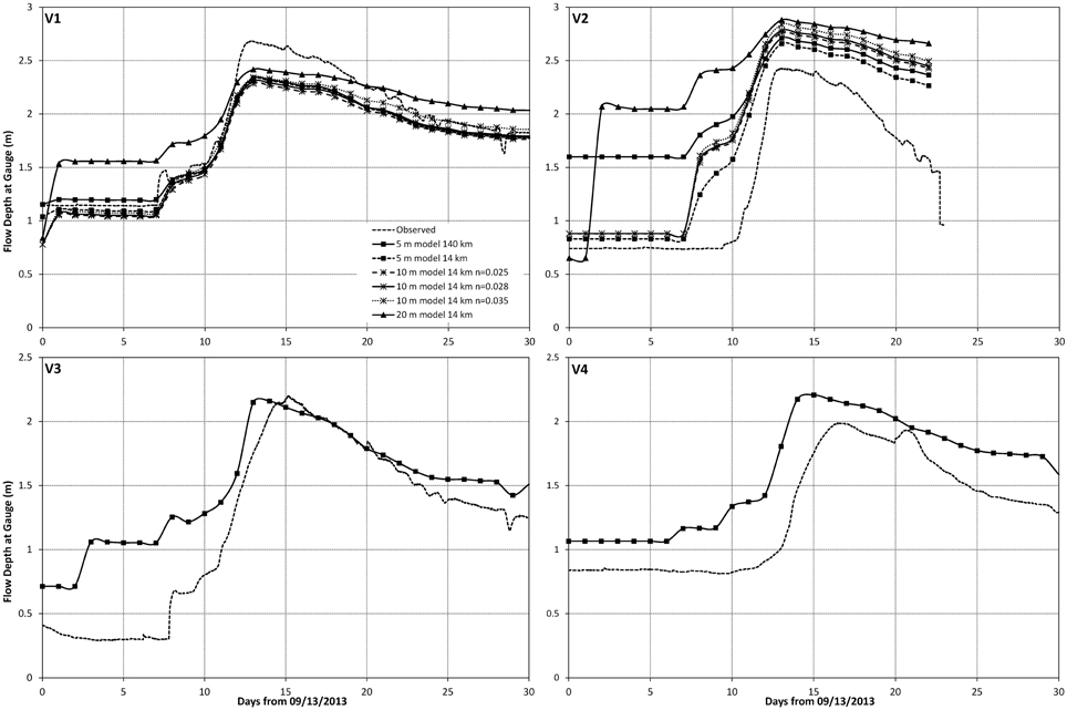
Figure 3. Observed vs. predicted flow at USGS gaging stations. Mesoscale models at gages (V1, V2), macroscale models at gages (V1–V4).

TABLE 3

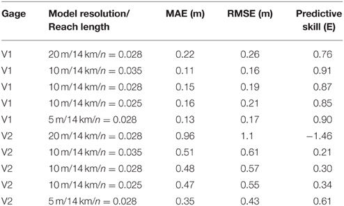
Table 3. Mean average error (MAE), Root mean square errors (RMSE), and Nash-Sutcliffe predictive skill of depth predictions at two gaging stations for the 14 km reach models at different resolution.

Figure 4 offers a closer look at the location of the gages, and more insight into the effect of mesh design on model predictions of flow. At both V1 and V2 the channel splits, whereby V1 is located on the northern branch and V2 on the southern branch of the split (Figure 4A). As the mesh is coarsened beyond 5 m resolution, these splits are no longer resolved resulting in a singular deeper channel at the same locations (Figure 4C). Figure 4 also shows that at 5 m resolution, the river is represented by many distinct channels separated by islands (Figure 4A), but as the mesh is coarsened to 10 m resolution (Figure 4B) and 20 m resolution (Figure 4C), the size and number of islands is reduced. Figure 3 shows that increasing mesh resolution leads to increasing peak flood stage prediction, so the trends shown in Figure 4 can be attributed to a combination of factors: (a) fewer channels resolved with mesh coarsening, and (b) higher flood stage prediction with mesh coarsening.

FIGURE 4

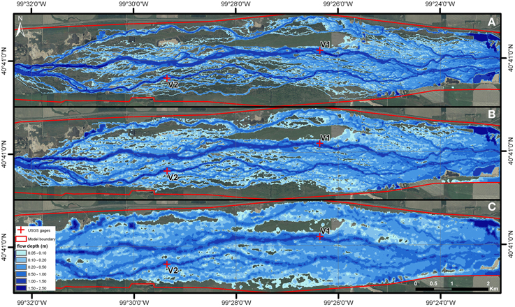
Figure 4. Predicted flow depth at peak flow (day 13) for mesoscale models at different resolutions. (A) 5 m, (B) 10 m, and (C) 20 m.

When the same resistance parameter is used (n = 0.028 m^1∕3 s), the 10 m mesoscale model is slightly less accurate (RMSE = 0.57 m) than the 5 m mesoscale model (RMSE = 0.43 m). However, Figure 3 shows that varying the resistance parameter between (n = 0.025 and 0.035 m^1∕3 s) can affect flood stage by up to about 10 cm at high flow stages, which is similar to the difference in stage predictions between the 5 and 10 m resolution models. Differences in stage errors due to resistance parameters are also shown in Table 3. It is noted that variable resistance has relatively little impact on stage under low flow conditions, i.e., prior to Day 7 of the simulation. It is also noted that increasing Manning n from 0.028 to 0.035 m^1∕3 s reduces errors in the main channel (gage V1) but increases errors in the smaller side-braid (gage V1), as shown in Table 3. This is counterintuitive considering that side braids tend to be more vegetated and would therefore warrant a larger resistance parameter. It cannot be ruled out that smaller resistance parameters improve accuracy in the side channel by absorbing errors in the 10 m resolution representation of topography.

To summarize, these results show that model predictions of stage are primarily sensitive to topographic modeling (mesh resolution) at low flood stages, and are sensitive to both topographic modeling and resistance parameters at high flow stages. Since the models are not calibrated it is not possible to determine which resolution and resistance parameterization performs best. However, considering the potential impact of mesh resolution on morphodynamics, a coarsening of mesh resolution would lead to an overprediction of flow across the floodplain, which in turn would negatively affect predictions of floodplain morphology. Therefore, for model application during moderate flow events, sufficient model resolution to resolve narrow braids is recommended. These results highlight the importance of validation data, and the need for spatially distributed stage and velocity data to untangle the relative contribution of different model errors including topographic errors, resistance parameter errors, and structural model errors.

Macroscale Flow Modeling

Application of the macroscale flow model at 5 m resolution reveals the variability in Platte River flow properties over the 140 km reach and across the 30 day simulation period. Figure 5 shows the average depth, total width, and total discharge for the river (integrated over all channels in the floodplain) at three time instances, 09/23/2013 00:00 am before arrival of the flood wave (Figure 5A), 09/26/2013 00:00 am at flood peak (Figure 5B) and 10/03/2013 00:00 am during flood recession (Figure 5C); these three instances will henceforth be referenced as pre-flood, peak-flood, and post-flood, respectively. The thin lines in Figure 5 correspond to cross-sectional averaged flow attributes, while the thick lines correspond to the reach-averaged flow attributes (over a length scale of 1 km, as described in the Materials and Methods section).

FIGURE 5

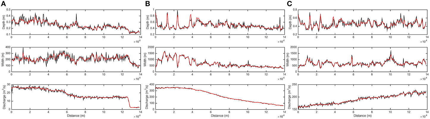
Figure 5. Reach-averaged flow attributes for (A) 09/23/2013, (B) 09/26/2013, and (C) 10/03/2013. The red line corresponds to reach averages data, while the black line corresponds to cross-sectional averages.

Figure 5 shows that river width increases roughly five fold with the passage of the flood and an order of magnitude increase in discharge (comparing pre-flood and peak-flood conditions in Figures 5A,B, respectively), while river depth is less sensitive to discharge. A striking feature of the river is the effect of embanked roadways that cross the floodplain; these create a channel constriction that increases channel depth locally. Localized maxima in channel depth can be seen under peak flow conditions (Figure 5B) at alongstream distances of roughly 13, 23, and 38 km.

Figure 6 shows the pre-flood, peak-flood and post-flood complexity of braiding at an 8 km reach near the town of Kearney, NE. Under pre-flood conditions, (Figure 6A), the number of active channels ranges from 1 to 5 and local flow depth varies from a few centimeters to 0.5 m. With peak-flood conditions (Figure 4B), local water depth increases up to 2.8 m and the entire floodplain becomes active in conveying the flood. When the flood recedes (Figure 6C), islands re-emerge and ponded water in local depressions is cut off from areas of channel flow. Drainage of this water is controlled by subsurface flow that is not presently incorporated into the model; this indicates that predictions during the falling limb of the hydrograph (e.g., Figure 5C) may over-predict flood width and flood extent.

FIGURE 6

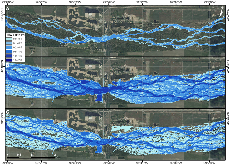
Figure 6. Modeled water depths for an 8 km reach of the Platte River near Kearney, NE, for (A) 09/23/2013, (B) 09/26/2013, and (C) 10/03/2013.

Figure 7 (top panels) shows that the water surface is nearly uniform along the length of the study reach and over the progression of the flood (linear trend line shown to emphasize this point). However, the model reveals significant transverse variability in water surface heights. Figure 7 (middle panels) shows the difference between flood height in individual channels and the cross-sectionally averaged flood height, which approach ±2 m. Leopold and Wolman (1957) reported that two channels in parallel in a BR can have significantly different water heights, and this result shows that mechanistic 2D models are capable of resolving such variability; this may be particularly important for investigations of subsurface transport because it points to subsurface transport perpendicular to the channel flow direction. Figure 7 (bottom panels) shows the number of distinct channels (defined by a depth tolerance of 5 cm) that exist at each cross-section during pre-flood, peak-flood and post-flood conditions. This shows that an increase in discharge can lead to an increase in the number of active channels, as primary channels are filled and secondary and tertiary channels on the floodplain are activated. On the other hand, an increase in discharge can also lead to a decrease in the number of channels when parallel channels merge. The relationship between the number of channels (also known as the braid index) and discharge is clearly complex.

FIGURE 7

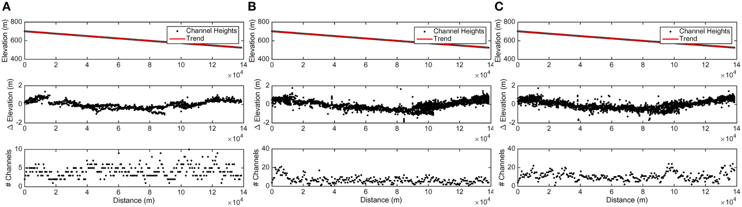
Figure 7. Predicted cross-sectional water surface elevations (top panels), cross-sectional water surface elevation range as given by different parallel channels (middle panels), and number of cross-sectional active channels (bottom panels), for (A) 09/23/2013, (B) 09/26/2013m and (C) 10/03/2013.

Flow attributes based on cross-sectional analysis (black lines in Figure 5) appear noisy compared to reach-averaged counterparts (red line in Figure 5), which is to some degree expected because the reach averaging process acts as a high frequency filter. High frequency noise (at spatial scales of a few km or less) in the spatial distribution of depth and width can be explained, at least in part, by the complexity of the flow paths through the system, which is shown in Figure 6. However, high frequency noise in the spatial distribution of discharge cannot be readily explained by braided flow complexity because discharge is a conserved quantity in the model, and variability should be consistent with boundary forcing, which involves gradual changes over time. Thus, high frequency noise is also attributed to a combination of the data structure of the flow solver and the post-processing of model data. The flow solver permits inconsistencies between the solution at cell edges and cell centers; discharge based on edge-base data is exactly conservative, whereas discharge based on cell centered data is not, and model output that is rasterized for post-processing is based on cell-centered data. Secondly, post-processing whereby unstructured data in triangles is converted into a raster format can also introduce errors in the velocity and depth which affect the level of conservation that can be achieved with post-processed data. In summary, while the flow model itself is exactly conservative on a cell-by-cell basis and by extension of the entire domain (to numerical precision), several factors associated with the output and post-processing of data introduce high frequency noise. The level of noise is negligible at scales greater than a few km, and therefore does not represent a significant drawback with respect to river analysis at mesoscales and macroscales, but it does suggest that errors may be present at the microscale and these should be kept in mind alongside other sources of uncertainty when model results are used for decision-making.

Figure 3 (solid lines with squares) shows how the macroscale model predictions of flood stage compare with measurements at USGS gages in the 140 km study domain shown in Figure 1.

Table 4 shows the uncalibrated results at each gage for the macroscale model. At gage V1, the MAE and RMSE are comparable to the accuracy of floodplain heights measured by aerial lidar (RMSE = 0.18 m), so this represents a high level of predictive skill (E = 0.91). At gage V2 (small side channel), the MAE, RMSE and predictive skill are large and Figure 6 indicates that the macroscale model is particularly inaccurate at low flood stages. This is curious since the same resolution model (5 m) at the mesoscale performs well at the same gage location. Upon further analysis we noticed slight differences in the connectivity of VIP nodes, caused by the meshing process, between the two models. This leads to small variations in channel geometry which can affect flow volumes, especially in small channels and during low flow conditions.

TABLE 4

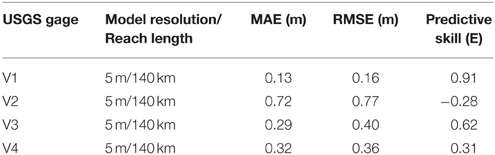
Table 4. Mean average error (MAE), Root mean square errors (RMSE), and Nash-Sutcliffe predictive skill of depth predictions at four gaging stations for the 140 km reach model.

Moving downstream to a point 40 km from the upstream boundary of the model (gage V3), the RMSE of the flood depth prediction is 0.40 m and the accuracy is particularly good at peak flood flow. Larger errors at low flow are likely a result of less accurate channel data. Finally at a distance of 110 km from the upstream boundary (gage V4), the RMSE of flood depth is 0.36 m which compares closely to the 0.39 m topographic error reported in Section Site Description and Available Data for the river channel in this reach. Overall, the accuracy of the height predictions is strongly linked to the accuracy of topographic data.

Figure 6 also points to a phase error in the flood wave prediction, because the predicted arrival time is increasingly ahead of its measured arrival time with downstream distance. This has a negative effect on the model predictive skill, which at gage V4 is half that of gage V3. This likely reveals either a limitation of the assumed model of flow resistance involving a spatially uniform Manning resistance coefficient or the effect of topographic features that aren't capture by the model. An increase in resistance would slow down the speed of the flood, which would increase accuracy at gage V4, but also increase the prediction of flood heights which would decrease accuracy at gage V4. This suggests that the task of calibration is not necessarily a simple one and achieving an improved model fit would likely demand calibration of both topographic data and resistance parameters.

Overall, the results shown in Figures 3–7 indicate that the model captures the spatiotemporal complexity of BR flows from microscales to macroscales. However, these results also highlight several limitations of the model that may deserve attention when applications of the model are used for decision-making; in particular, (1) the inability to account for subsurface flow, which affects drainage of ponded floodplains during flood recession, (2) uncertainty in predictions linked to uncertain topography and resistance parameters, and (3) uncertainty that may be introduced by post-processing of model data.

Hydraulic Geometry

The power law coefficients and exponents fitted with R² > 0.70 are shown in Figure 8. A fitness threshold was used to filter out stations associated with development, such as embankments and ponds, where river shape is no longer dominated by natural processes. Additionally, a flow threshold of 0.4 m³/s was introduced to filter out individual samples of channel flows corresponding to relatively stagnant water; such channels were observed predominantly during flood recession because side channels are cut off from areas of active flow. This filtering yielded 122 stations for analysis with the AHG-D method and 230 stations for the AHG-I method. Figure 8 also shows the timewise minimum, maximum and average discharge over the flood event vs. alongstream distance, which indicates that each cross-section experienced nearly the same range of flow conditions, although a minor attenuation in the average discharge is evident and interpreted as a model prediction of floodwave attenuation in the absence of significant lateral inflows. Also shown is the timewise minimum, maximum and average braid index (BI) defined by the number of flow-active channels in parallel at a cross-section. This reveals significant spatial and temporal variability in the BI with values ranging from 1 to 15. BI differs from the number of channels shown in Figure 7 (which range from 1 to 25) because the latter includes cases of stagnant water. Note that a minimum BI = 0 is shown near the downstream end of the river reach, but this is an artifact of the model initialization process which involved an initially dry channel and a multi-day period to initially wet the channel (not long enough to reach the downstream boundary). Also note that a maximum BI of only one or two channels occurs where the floodplain is constricted by development (i.e., bridge crossings).

FIGURE 8

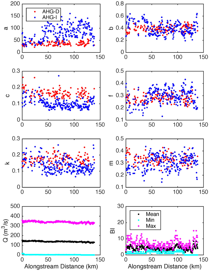
Figure 8. Variability of hydraulic geometry power law coefficients (a, c, k) and exponents (b, f, m) along the modeled reach. Top panels represent the coefficient/exponent terms related to depth, second row related to width and third row related to velocity. Bottom panels show the alongstream variability in discharge and braid index (BI).

The HG results point to a remarkably simple model of river hydraulics for this complex system characterized by spatially uniform AHG parameter distributions for width, depth and velocity. Figure 8, in particular, points to a uniform spatial distribution of AHG-D parameters, while the spatial distribution of AHG-I parameters exhibits signs of a spatial trend and notably greater variability. The mean and standard deviation of parameter values resulting from both methods are shown in Table 5, and AHG-I values are consistently larger than the corresponding AHG-D values. The mean parameter values are also different between AHG-D and AHG-I in all cases (paired t-test at 5% significance level) except the width exponent b.

TABLE 5

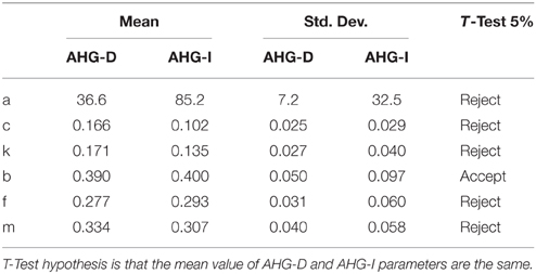
Table 5. Comparison of AHG coefficients and exponents.

Figure 9 presents a ternary diagram of the AHG-D (red) and AHG-I (blue) exponents. This graphically illustrates that depth and velocity share a similar sensitivity to discharge, but that river width exhibits a stronger sensitivity to discharge. Additionally, greater scatter in AHG-I exponents compared to AHG-D illustrates the larger standard deviation in parameter values reported in Table 5.

FIGURE 9

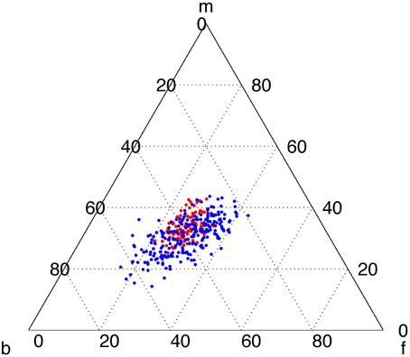
Figure 9. Ternary diagram of AHG exponents. AHG-D shown in red and AHG-I in blue.

These results indicate that when the river is conceptualized as a single channel with effective properties (AHG-I), there is greater spatial variability in HG than when the river is modeled as a multi-channel system (AHG-D). Perhaps surprisingly, the HG of the river is preserved despite significant changes to its braided configuration (cf. Figure 8). However, this finding is not inconsistent with previously reported expectations for downstream consistency in AHG (e.g., Rhodes, 1977).

Figures 10, 11 explore the effects of grid resolution and surface resistance on the HG of the Platte River as given by the mesoscale models. Figure 10A shows that an increase in resolution from 5 to 20 m leads to a whole unit increase (one channel) of the flood-average BI. Figures 10B,C show the effect on hydraulic geometry (AHG-I) coefficients. Focusing first on channel width (Figure 10B), the 20 m model leads to larger AHG-I coefficients and smaller exponents compared to the finer resolution models. The differences between the 10 and 5 m resolution models are noticeably smaller and mainly characterized by a difference in the exponent, b. Focusing now on channel depth (Figure 10C), grid resolution appears to mainly effect the coefficient, f, which is reflected by a vertical offset of the data across model resolutions. Finally, focus on velocity shows that grid resolution has a strong effect on both the coefficient k and the exponent m. An increase in model resolution leads to an increase in k and a decrease in m. Collectively, these trends point to the effect of grid refinement as a decrease in channel width and an increase in channel velocity. A similar trend in channel velocity is reported by Williams et al. (2013).

FIGURE 10

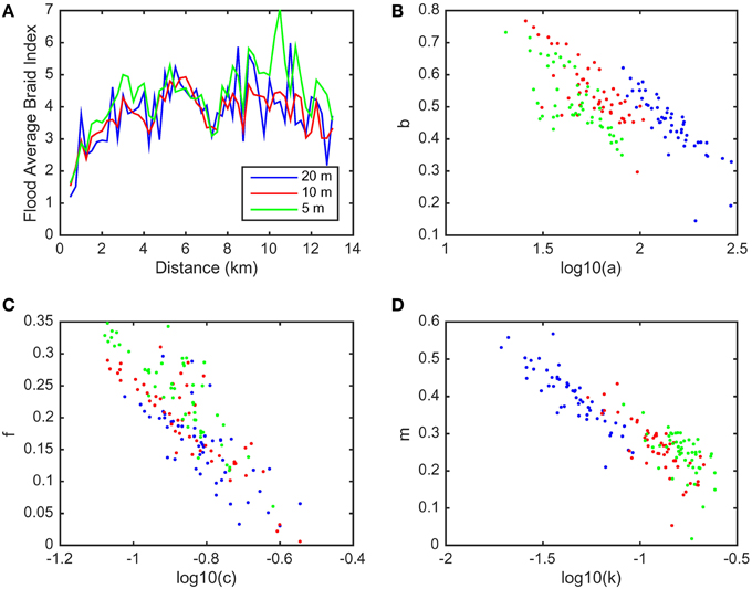
Figure 10. Effect of mesh resolution on hydraulic geometry coefficients and exponents. (A) Braid Index, (B) width (a,b), (C) depth (c,f), and (D) velocity (k,m).

FIGURE 11

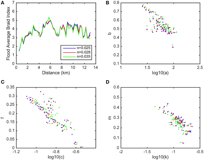
Figure 11. Effect of surface resistance on hydraulic geometry coefficients and exponents. (A) Braid Index, (B) width (a,b), (C) depth (c,f), and (D) velocity (k,m).

Figure 11 reveals the effect of flow resistance on HG. Figure 11A shows that an increase in Manning n from 0.025 to 0.035 leads to a relatively small change in the flood-average BI of at most 0.3 or about 6%. Figure 11A also shows that increasing Manning n can both increase and decrease the BI, depending on location. Figures 11B–D show the effect of increasing Manning n on HG coefficients and exponents. The strongest responses are an increase in c (Figure 11C) and a decrease in k (Figure 11D) which point to deeper and slower flows, respectively. Weaker responses include an increase in b (Figure 11B), a decrease in f (Figure 11C), and a decrease in m (Figure 11D). Overall, these trends indicate that over the range of Manning n-values considered, an increase in Manning n causes channels to widen at a slightly faster rate (weak increase in b) and to have deeper and slower low flows (increase in c, decrease in k).

Hydraulic Habitat Classification

Figure S4 shows the frequency of river depth and velocity predicted by macroscale model, and lines indicating the depth and velocity breaks that define four hypothetical habitat types: deep pools (upper left), deep runs (upper right), shallow pools (lower left), and shallow runs (lower right). The velocity break is 0.45 m/s and was selected first because this approximately bounds a cluster of deep (~2 m), slow moving water. A depth break of 0.6 m was selected second because this separates high frequency shallow pools (red and yellow colors) from relatively low frequency (green and blue colors) deep pools. These breaks are similar to values used in previous studies. For example, Wyrick et al. (2014) used a velocity break of 0.3 and 0.6 m to constrain pools at two different sites in California. Jowett (1993) found a velocity of 0.56 m/s constrained runs, and Wyrick et al. (2014) differentiated a run from a pool by a velocity of 0.6 m/s. Nevertheless, it should be stressed that because the classification used here is completely data driven, it is not reflective of the actual morphological units of the Platte River that would be mapped by a field investigation of flow and sediment.

Figure 12 presents the spatial distribution of depth (Figure 12A), velocity (Figure 12B) and classified hydraulic habitat types (Figure 12D) for a short reach of the Platte River at a high flow condition. Additionally, Figure 12C shows the habitat distribution from a depth-velocity classification with smaller break values given by 0.30 m/s and 0.54 m. Similar to the findings of Jowett (1993), deep pools are consistently mapped (Figures 12C,D) since they are characterized by the intuitive combination of slow moving and deep water. The deep pools were primarily located near man-made roads and detention ponds and represented the smallest proportion of hydraulic habitat along the reach for all the daily time outputs. Shallow runs are commonly surrounded by deep runs, and deep runs occur in the widest channels. Figure S4 shows that shallow pools are the most frequently occurring habit, and if the velocity break of 0.45 m/s is reduced there would be a significant increase in shallow run habitat. This result is apparent in Figure 12C where more of the braid network is classified as shallow run habitat compared to Figure 12D.

FIGURE 12

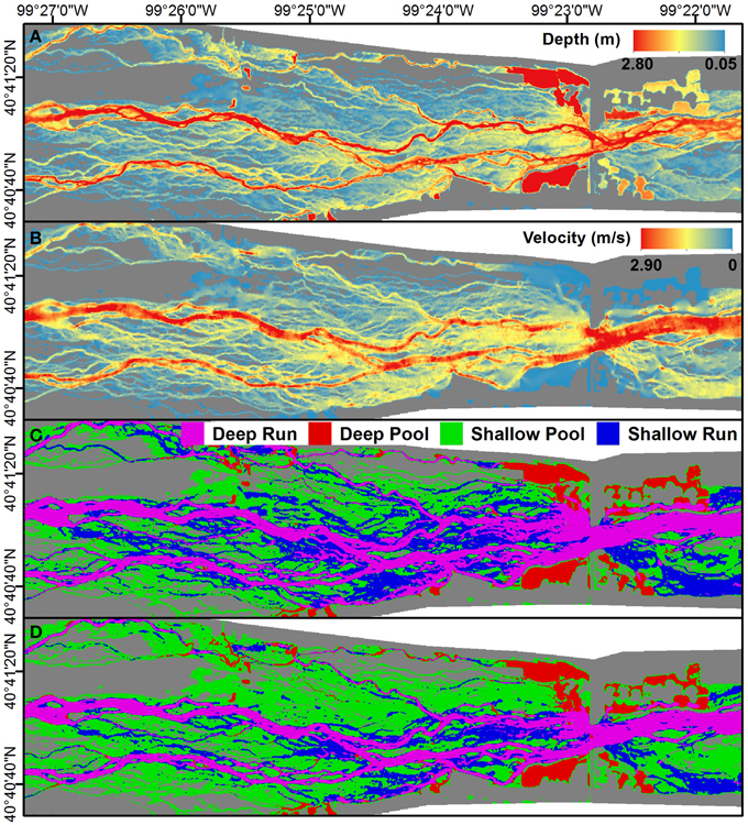
Figure 12. Example of habitat classification using velocity and depth raster data for day 9/27/15. (A) depth raster, (B) velocity raster, (C) classification system with breaks at velocity of 0.30 m/s and a depth of 0.5 m, (D) classification system with breaks at a velocity of 0.45 m/s and a depth of 0.6 m.

The macroscale evolution of hydraulic habitat over the course of a flood is revealed by processing daily model output over the entire study area. Figure 13 presents habitat width at daily time intervals, as well as the sensitivity of habitat width to the velocity and depth breaks used for classification. Habitat width is calculated as the total habitat area at the macroscale divided by the length of the reach. In addition to the four aquatic habitats defined by the classification system shown in Figure S4, a fifth habitat corresponding to subaerial floodplain is also shown since this is critical to several bird species. Figure 13 shows that all of the hydraulic habitats increase with the rising limb of the flood, with a commensurate decrease in subaerial floodplain habitat. An increase in shallow habitats resulting from an increase in discharge may not be intuitive but is explained by a river system that rapidly expands in width with an increase in discharge. Figure 13 also shows the sensitivity of habitats to the break values used for classification. Increasing the break values for both velocity and depth increases the width of shallow pools, decreases the width of deep runs, and decreases the width of shallow runs but has relatively little impact on deep pools.

FIGURE 13

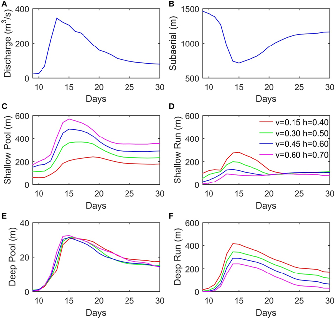
Figure 13. Average cross sectional widths of habitats for daily raster data. Calculated as habitat area divided by length of river reach. (A) Reach averaged discharge for 1 km reach near upstream boundary, (B) subaerial or dry habitat, (C) shallow pool habitat, (D) shallow run habitat, (E) deep pool habitat, (F) deep run habitat. Different colored lines represent different break values used for habitat classification.

Figure 14 shows the sensitivity of hydraulic habitat width to grid resolution based on mesoscale simulations. Figure 14A shows discharge into the reach resolved at three separate grid resolutions based on a 1 km reach-averaged discharge at a cross-section 500 m downstream of the upstream boundary, and reveals the expected consistency. The sensitivity of habitat width to grid resolution is striking as shown in Figures 14B–F. As the grid is coarsened, the model predicts far more pool habitat (Figures 14C, E) and a proportional decrease in subaerial habitat (Figure 14B). Run habitat is not as sensitive to resolution as pool habitat, particular at the peak of the flood (days 12–13). However, Figure 14D shows that the 5 m resolution model predicts shallow run habitat at low flows (Days 7–12) that is not predicted by the 20 m resolution model.

FIGURE 14

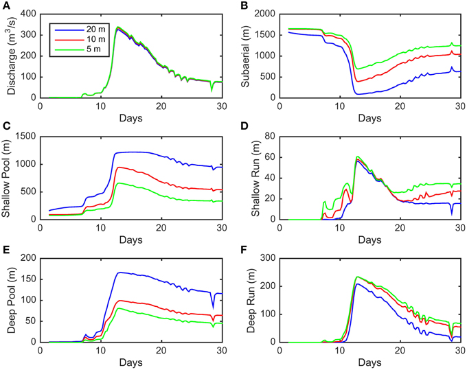
Figure 14. Effect of mesh resolution on habitat classification. (A) Effect on discharge, (B) subaerial habitat, (C) shallow pool habitat, (D) shallow run habitat, (E) deep pool habitat, and (F) deep run habitat.

The sensitivity of habitat width to flow resistance is presented in Figure 15. Figure 15A again shows that discharge is consistent, in this case across the three runs with different levels of flow resistance. Figures 15B–F show that a shift to a greater Manning n-value leads to a decrease in shallow run habitat (Figure S2D) while there is virtually no impact on deep run habitat (Figure 15F). An increase in Manning n also causes an increase in both shallow pool (Figure 15C) and deep pool (Figure 15E) habitat, and a decrease in subaerial habitat (Figure 15B).

FIGURE 15

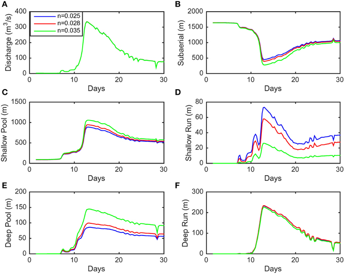
Figure 15. Effect of surface resistance on habitat classification. (A) Effect on discharge, (B) subaerial habitat, (C) shallow pool habitat, (D) shallow run habitat, (E) deep pool habitat, and (F) deep run habitat.

The preceding results show that hydraulic habitat distributions predicted by hydrodynamic models and a simple classification scheme can be affected by several factors: habitat break values, grid resolution and resistance parameters. These findings not only emphasize the need for local field work to develop a classification scheme, but the importance of validating the accuracy of hydrodynamic model predictions within all habitat types.

Conclusion

An automated unstructured grid generation technique is presented for efficient metric-resolution modeling of a BR at mesoscales to macroscales. Automation is achieved by using point constraints instead of breakline constraints as input to constrained Delaunay grid generation software. Point constraints are automatically identified by processing a DTM for VIPs, whereas breakline constraints require a high level of time-consuming, manual delineation. The vertical accuracy of model grids of the braided Platte River in central Nebraska, USA created with either point constraints or breakline constraints are found to be equal at the mesoscale. Hence, the benefit of the proposed method is automation which radically expedites model setup and enables the creation of a 5 m resolution macroscale grid of the Platte River which would be virtually impossible to set up manually. The macroscale model shows good predictive skill at several gages where flow observations were made, and errors in predicted flow depths track errors in the topographic data.

A mesoscale analysis justifies the choice of a 5 m resolution grid for macroscale modeling based on topographic errors; the vertical accuracy of the 5 m resolution unstructured grid models is no worse than the measurement accuracy while the vertical accuracy of 10 m and 20 m resolution unstructured grids is greater than measurement accuracy. The Platte River is characterized by a main thread 50–100 m wide and side threads as fine as 10 m, so use of a grid coarser than 10 m filters out significant channel features and this explains the increase in vertical error. A 5 m resolution grid is also justified by modeling “best practices” which call for a grid fine enough to resolve all scales of interest. Based on the mesoscale analysis, it may be possible to calibrate a 10 m resolution model to match observed gage measurements, but differences in the representation of channel networks are likely as shown in Figure 4.

Grid coarsening from 5 m resolution to 10 and 20 m resolution leads to an increase in river width, an increase in average river depth, and a decrease in the average river velocity. These changes are also reflected in HG analysis, and in the predicted distribution of four hydraulic habitat types: deep pools, shallow pools, deep runs, and shallow runs. Differences in stage caused by grid coarsening are magnified in relatively smaller side channels compared to the main channel. Changes in resistance parameters also lead to predictions characterized by greater width and depth and a smaller velocity. These results emphasize the need to calibrate hydrodynamic models and validate spatially distributed predictions of both river stage and velocity. Remote sensing techniques could prove invaluable for acquiring the spatial distribution of flow attributes. As a first step, NASA's SWOT mission is designed to measure the hydraulic properties of medium to large rivers such as reach average flow width and height and to outline the spatial extent of inundation, which would be complementary to conventional gage measurements in the Platte River and would assist with model calibration.

Macroscale hydrodynamic modeling is shown to generate a wealth of data that can be processed for hydrological, morphological and ecological analysis. For example, model data are processed to analyze two forms of AHG including a distributed form (AHG-D) that considers each channel in parallel at a cross-section separately and an integrated form (AHG-I) that is based on cross-sectionally averaged properties. AHG-I analysis reveals more spatial variability in river geometry than AHG-D. Analysis of river hydraulic habitat is also shown as a demonstration, and results highlight that uncertainty in habitat predictions that can arise from several sources and emphasize the need for site specific validation.

This study also brings to light several model limitations that need to be considered when metric resolution macro-scale hydraulic models are applied for decision making. First, models are likely to overpredict flood extents after the passage of the flood wave since subsurface flow, which is an important driver of floodplain drainage, is generally not considered in hydraulic modeling. Second, errors in topographic data and uncertainties in surface resistance values used for model parameterization directly affect simulation results. Not considering channel morphodynamics further limits the application of fine resolution models to small to moderate flow events, since extreme events have the ability to majorly impact channel and floodplain geometries. For this reason it is recommended to use topographic data which has the closest temporal correlation to the event being modeled, and to calibrate the model using stage and velocity measurements as well as observed flow widths if available. Post large flow events, fine resolution models should be updated with new data to account for potential morphological changes in the system. Third, there may be a loss of fine scale information when unstructured grid hydrodynamic model data are transformed to raster grids due to interpolation errors and the model data structure, i.e., inconsistencies in cell and edge-based variable values. This motivates basic continuity checks of model output.

Conflict of Interest Statement

The authors declare that the research was conducted in the absence of any commercial or financial relationships that could be construed as a potential conflict of interest.

Acknowledgments

This modeling framework was motivated by the desire to undertake large-scale metric-resolution hydraulic modeling to study the performance of the upcoming NASA SWOT mission over complex braided streams. As such we would like to thank the NASA SWOT science definition team for their input into the development of the model and NASA for funding the project (grant # NNX13AE21G). Our special thanks also go to the Platte River Recovery Implementation Program Executive Director, Jerry Kenny, and Director of Habitat Management and Rehabilitation, Jason Farnsworth, for graciously providing numerous geospatial data products, which were instrumental in parameterizing and validating the Platte river hydraulic model.

Supplementary Material

The Supplementary Material for this article can be found online at: https://www.frontiersin.org/article/10.3389/feart.2015.00074

Figure S1. Flow properties at USGS gage I1 for 2013 high flow event. Vertical lines indicate dates of flow conditions sampling (midnight) for data analysis.

Figure S2. Discharge cumulative distribution function for gage I1 based on flow data from 10/01/1930 to 03/15/2015. Vertical gray lines indicate lower (left) and upper (right) boundaries of flows recorded during the 2013 high flow event.

Figure S3. (A) Original 1 m DTM, (B) VIP TIN, (C) VIP TIN mesh.

Figure S4. Hydraulic variables from daily raster data for days 9 through 30 from 9/13/2013. The habitat classes of deep run, deep pool, shallow run, and shallow pool are defined by the upper right, upper left, lower right, and lower left sections of each plot. The color of each pixel inside the plots represents the number of raster cells that fall within its area. Only raster cells with a depth >5 cm are considered.

References

Abu-Aly, T. R., Pasternack, G. B., Wyrick, J. R., Barker, R., Massa, D., and Johnson, T. (2014). Effects of LiDAR-derived, spatially distributed vegetation roughness on two-dimensional hydraulics in a gravel-cobble river at flows of 0.2 to 20 times bankfull. Geomorphology 206, 468–482. doi: 10.1016/j.geomorph.2013.10.017

CrossRef Full Text | Google Scholar

Acrement, G. J., and Schneider, V. R. (1984). Guide for Selecting Manning's Roughness Coefficients for Natural Channels and Flood Plains. U.S. Geological Survey Water-Supply Paper 2339.

Ayers Associates Olsson Associates (2009). Channel Geomorphology and In-Channel Vegetation Monitoring of the Central Platte River - Year 1 (2009). Fort Collins, CO: Colo.

Bates, P. D. (2012). Integrating remote sensing data with flood inundation models: how far have we got? Hydrol. Process. 26, 1515–2521. doi: 10.1002/hyp.9374

CrossRef Full Text | Google Scholar

Begnudelli, L., and Sanders, B. F. (2007). Conservative wetting and drying methodology for quadrilateral grid finite volume models. ASCE J. Hydr. Eng. 133, 312–322. doi: 10.1061/(ASCE)0733-9429(2007)133:3(312)

CrossRef Full Text | Google Scholar

Begnudelli, L., Sanders, B. F., and Bradford, S. F. (2008). Adaptive Godunov-based model for flood simulation. ASCE J. Hydr. Eng. 134, 714–725. doi: 10.1061/(ASCE)0733-9429(2008)134:6(714)

CrossRef Full Text | Google Scholar

Begnudelli, L., Valiani, A., and Sanders, B. F. (2010). A balanced treatment of secondary currents, turbulence and dispersion in a depth-integrated hydrodynamic and bed deformation model for channel bends. Adv. Water Resour. 33, 17–33. doi: 10.1016/j.advwatres.2009.10.004

CrossRef Full Text | Google Scholar

Bowen, Z. H., Bovee, K. D., and Waddle, T. J. (2003). Effects of flow regulation on shallow-water habitat dynamics and floodplain connectivity. Trans. Am. Fish. Soc. 132, 809–823. doi: 10.1577/T02-079

CrossRef Full Text | Google Scholar

Clifford, N. J., Wright, N. G., Harvey, G., Gurnell, A. M., Harmar, O. P., and Soar, P. J. (2010). Numerical modeling of river flow for ecohydraulic applications: some experience with velocity characterization in field and simulated data. J. Hydraul. Eng. 136, 1033–1041. doi: 10.1061/(ASCE)HY.1943-7900.0000057

CrossRef Full Text | Google Scholar

Condon, S. M. (2005). Geologic Studies of the Platte River, South-Central Nebraska and Adjacent Areas—Geologic Maps, Subsurface Study, and Geologic History. U.S. Geological Survey Professional Paper 1706.

Google Scholar

Cook, A., and Merwade, V. (2009). Effect of topographic data, geometric configuration and modeling approach on flood inundation mapping. J. Hydrol. 377, 131–142. doi: 10.1016/j.jhydrol.2009.08.015

CrossRef Full Text | Google Scholar

Costabile, P., and Macchione, F. (2015). Enhancing river model set-up for 2-D dynamic flood modelling. Environ. Model. Softw. 67, 89–107. doi: 10.1016/j.envsoft.2015.01.009

CrossRef Full Text | Google Scholar

Crowder, D. W., and Diplas, P. (2000). Using two-dimensional hydrodynamic models at scales of ecological importance. J. Hydrol. 230, 172–191. doi: 10.1016/S0022-1694(00)00177-3

CrossRef Full Text | Google Scholar

Cunge, J. A., Holly, F. M. Jr., and Verwey, A. (1980). Practical Aspects of Computational River Hydraulics. Marshfield, WI: Pitman Publishing.

Google Scholar

Dewberry (2010). LiDAR Quality Assurance Final Report, Sub-project 1: Platte River Corridor Nebraska/Kansas LiDAR. Fairfax, VA.

Dottori, F., Di Balassarre, G., and Todini, E. (2013). Detailed data is welcome, but with a pinch of salt: accuracy, precision and uncertainty in flood inundation modeling. Water Resour. Res. 49, 6079–6085. doi: 10.1002/wrcr.20406

CrossRef Full Text | Google Scholar

Eakins, B. W., and Taylor, L. A. (2010). “Seamlessly integrating bathymetric and topographic data to support tsunami modeling and forecasting efforts,” in Ocean Globe, ed J. Breman (Redlands, CA: ESRI Press), 37–56.

Fernandez-Diaz, J. C., Glennie, C. L., Carter, W. E., Shrestha, R. L., Sartori, M. P., Singhania, A., et al. (2014). Early results from a simultaneous airborne terrain and shallow water bathymetry mapping LiDAR sensor. IEEE J. Sel. Top. Appl. Earth Obs. Remote Sens. 7, 623–635. doi: 10.1109/JSTARS.2013.2265255

CrossRef Full Text

Gallegos, H. A., Schubert, J. E., and Sanders, B. F. (2009). Two-dimensional, high-resolution modeling of urban dam-break flooding: a case study of Baldwin Hills, California. Adv. Water Resour. 32, 1323–1335. doi: 10.1016/j.advwatres.2009.05.008

CrossRef Full Text | Google Scholar

Gallien, T. W., Schubert, J. E., and Sanders, B. F. (2011). Predicting tidal flooding of urbanized embayments: a modeling framework and data requirements. Coast. Eng. 58, 567–577. doi: 10.1016/j.coastaleng.2011.01.011

CrossRef Full Text | Google Scholar

Gesch, D. B., Oimoen, M. J., and Evans, G. A. (2014). Accuracy Assessment of the U.S. Geological Survey National Elevation Dataset, and Comparison with Other Large-Area Elevation Datasets - SRTM and ASTER. U.S. Geological Survey Open-File Report 2014-1008.

Google Scholar

Gleason, C. J. (2015). Hydraulic geometry of natural rivers: a review and future directions. Prog. Phys. Geogr. 39, 337–360. doi: 10.1177/0309133314567584

CrossRef Full Text | Google Scholar

Gleason, C. J., and Smith, L. S. (2014). Toward global mapping of river discharge using satellite images and at-many-stations hydraulic geometry. Proc. Natl. Acad. Sci. U.S.A. 111, 4788–4791. doi: 10.1073/pnas.1317606111

PubMed Abstract | CrossRef Full Text | Google Scholar

Gonzalez, R. L., and Pasternack, G. B. (2015). Re-envisioning cross-sectional hydraulic geometry as spatially explicit hydraulic topography. Geomorphology 246, 394–406. doi: 10.1016/j.geomorph.2015.06.024

CrossRef Full Text | Google Scholar

Javernick, L., Hicks, D. M., Measures, R., Caruso, B., and Brasington, J. (2015). Numerical modelling of braided rivers with structure-from-motion-derived terrain models. River Res. Appl. doi: 10.1002/rra.2918. [Epub ahead of print].

CrossRef Full Text | Google Scholar

Jowett, I. G. (1993). A method for objectively identifying pool, run, and riffle habitats from physical measurements. N.Z. J. Mar. Freshwater Res. 27, 241–248. doi: 10.1080/00288330.1993.9516563

CrossRef Full Text | Google Scholar

Jowett, I. G. (1998). Hydraulic geometry of New Zealand rivers and its use as a preliminary method of habitat assessment. Regul. Rivers 14, 451–466.

Google Scholar

Karypis, G., and Kumar, V. (1999). Parallel multilevel k-way partitioning scheme for irregular graphs. SIAM Rev. 41, 278–300. doi: 10.1137/S0036144598334138

CrossRef Full Text | Google Scholar

Kim, B. H., Sanders, B. F., Schubert, J. E., and Famiglietti, J. S. (2014). Mesh type tradeoffs in 2D hydrodynamic modeling of flooding with a Godunov-based flow solver. Adv. Water Resour. 68, 42–61. doi: 10.1016/j.advwatres.2014.02.013

CrossRef Full Text | Google Scholar

Kinzel, P. J. (2008). River Channel Topographic Surveys Collected Prior to and Following Elevated Flows in the Central Platte River, Nebraska, Spring 2008. U.S. Geological Survey Data Series 380.

Google Scholar

Kinzel, P. J., Nelson, J. M., and Heckman, A. K. (2006). Channel Morphology and Bed-Sediment Characteristics Before and After Riparian Vegetation Clearing in the Cottonwood Ranch, Platte River, Nebraska, Water Years 2001–2004. U.S. Geological Survey Scientific Investigations Report 2005–5285.

Kinzel, P. J., and Runge, J. T. (2010). Summary of Bed-Sediment Measurements Along the Platte River, Nebraska, 1931–2009. U.S. Geological Survey Fact Sheet 2010–3087.

Lane, S. N., Bradbook, K. F., Richards, K. S., Biron, P. A., and Roy, A. G. (1999). The application of computational fluid dynamics to natural river channels: three-dimensional versus two-dimensional approaches. Geomorphology 29, 1–20. doi: 10.1016/S0169-555X(99)00003-3

CrossRef Full Text | Google Scholar

Lee, J. (1991). Comparison of existing methods for building triangular irregular network models of terrain from grid digital elevation models. Int. J. Geogr. Inform. Sci. 5, 267–285. doi: 10.1080/02693799108927855

CrossRef Full Text | Google Scholar

Legleiter, C. J., and Goodchild, M. F. (2005). Alternative representations of in−stream habitat: classification using remote sensing, hydraulic modeling, and fuzzy logic. Int. J. Geogr. Inform. Sci. 19, 29–50. doi: 10.1080/13658810412331280220

CrossRef Full Text | Google Scholar

Leopold, L. B., and Maddock, T. Jr. (1953). The Hydraulic Geometry of Stream Channels and Some Physiographic Implications. U.S. Geological Survey Professional Paper 252.

Google Scholar

Leopold, L. B., and Wolman, M. G. (1957). River Channel Patterns: Braided, Meandering, and Straight. Washington, DC: U.S. Geological Survey Professional Paper 282–B.

Li, Z., Zhu, Q., and Gold, C. (2005). Digital Terrain Modeling, Principles and Methodology. Boca Raton, FL: CRC Press.

Google Scholar

Maune, D. F. (ed.). (2001). Digital Elevation Model Technologies and Applications: The DEM Users Manual. Bethesda, MD: ASPRS Publications.

Moir, H. J., and Pasternack, G. B. (2008). Relationships between mesoscale morphological units, stream hydraulics and Chinook salmon (Oncorhynchus tshawytscha) spawning habitat on the Lower Yuba River, California. Geomorphology 100, 527–548. doi: 10.1016/j.geomorph.2008.02.001

CrossRef Full Text | Google Scholar

Neal, J., Schumann, G., and Bates, P. (2012). A subgrid channel model for simulating river hydraulics and floodplain inundation over large and data sparse areas. Water Resour. Res. 48, W11506. doi: 10.1029/2012WR012514

CrossRef Full Text | Google Scholar

Peucker, T. K., Flower, R. L., Little, J. J., and Mark, D. M. (1976). Digital Representation of Three-Dimensional Surfaces by Triangulated Irregular Networks (TIN). Technical Report Number 10, United State Office of Naval Research, Geography Programs.

Rhodes, D. D. (1977). The bfm diagram; graphical representation and interpretation of at-a-station hydraulic geometry. Am. J. Sci. 277, 73–96. doi: 10.2475/ajs.277.1.73

CrossRef Full Text | Google Scholar

Sanders, B. F. (2007). Evaluation of on-line DEMs for flood inundation modeling. Adv. Water Resour. 30, 1831–1843. doi: 10.1016/j.advwatres.2007.02.005

CrossRef Full Text | Google Scholar

Sanders, B. F. (2008). Integration of a shallow-water model with a local time step. J. Hydr. Res. 46, 466–475. doi: 10.3826/jhr.2008

CrossRef Full Text | Google Scholar

Sanders, B. F., Schubert, J. E., and Detwiler, R. L. (2010). ParBreZo: a parallel, unstructured grid, Godunov-type, shallow-water code for high-resolution flood inundation modeling at the regional scale. Adv. Water Resour. 33, 1456–1467. doi: 10.1016/j.advwatres.2010.07.007

CrossRef Full Text | Google Scholar

Sanford, J. P. (2007). Dam Regulation Effects on Sand Bar Migration on the Missouri River: Southeastern South Dakota. Master Thesis, Montana State University. Available online at: http://etd.lib.umt.edu/theses/available/etd-09062007-094840/unrestricted/Sanford,John.pdf (Accessed October 23, 2015).

Schubert, J. E., and Sanders, B. F. (2012). Building treatments for urban flood inundation models and implications for predictive skill and modeling efficiency. Adv. Water Resour. 41, 49–64. doi: 10.1016/j.advwatres.2012.02.012

CrossRef Full Text | Google Scholar

Schubert, J. E., Sanders, B. F., Smith, M. J., and Wright, N. G. (2008). Unstructured mesh generation and landcover-based resistance for hydrodynamic modeling of urban flooding. Adv. Water Resour. 31, 1603–1621. doi: 10.1016/j.advwatres.2008.07.012

CrossRef Full Text | Google Scholar

Schumann, G., Bates, P. D., Horritt, M. S., Matgen, P., and Pappenberger, F. (2009). Progress in integration of remote sensing–derived flood extent and stage data and hydraulic models. Rev. Geophys. 47:RG4001. doi: 10.1029/2008RG000274

CrossRef Full Text | Google Scholar

Schumann, G. J. P., Andreadis, K. M., and Bates, P. D. (2014). Downscaling coarse grid hydrodynamic model simulations over large domains. J. Hydrol. 508, 289–298. doi: 10.1016/j.jhydrol.2013.08.051

CrossRef Full Text | Google Scholar

Shen, Y., and Diplas, P. (2008). Application of two- and three-dimensional computational fluid dynamics models to complex ecological stream flows. J. Hydrol. 348, 195–214. doi: 10.1016/j.jhydrol.2007.09.060

CrossRef Full Text | Google Scholar

Shewchuk, J. R. (1996). “Triangle: engineering a 2D quality mesh generator and Delaunay triangulator,” in Applied Computational Geometry: Towards Geometric Engineering. Lecture Notes in Computer Science, Vol. 1148, eds M. C Lin and D. Manocha (Berlin: Springer-Verlag), 203–222. doi: 10.1007/BFb0014497

CrossRef Full Text | Google Scholar

Tsai, V. J. D. (1993). Delaunay triangulations in TIN creation: an overview and a linear-time algorithm. Int. J. Geogr. Inform. Sci. 7, 501–524. doi: 10.1080/02693799308901979

CrossRef Full Text | Google Scholar

Vivoni, E., Ivanov, V., Bras, R., and Entekhabi, D. (2004). Generation of triangulated irregular networks based on hydrological similarity. J. Hydrol. Eng. 9, 288–302. doi: 10.1061/(ASCE)1084-0699(2004)9:4(288)

CrossRef Full Text | Google Scholar

Williams, R. D., Brasington, J., Hicks, M., Measures, R., Rennie, C. D., and Vericat, D. (2013). Hydraulic validation of two-dimensional simulations of braided river flow with spatially continuous aDcp data. Water Resour. Res. 49, 5183–5205. doi: 10.1002/wrcr.20391

CrossRef Full Text | Google Scholar

Wu, W. (2007). Computational River Hydraulic. CRC Press.

Wyrick, J. R., Senter, A. E., and Pasternack, G. B. (2014). Revealing the natural complexity of fluvial morphology through 2D hydrodynamic delineation of river landforms. Geomorphology 210, 14–22. doi: 10.1016/j.geomorph.2013.12.013

CrossRef Full Text | Google Scholar

Yan, K., Di Baldassarre, G., Solomatine, D. P., and Schumann, G. J. P. (2015a). A review of low-cost space-born data for flood modelling: topography, flood extent and water level. Hydrol. Process. 29, 3368–3387. doi: 10.1002/hyp.10449

CrossRef Full Text | Google Scholar

Yan, K., Tarpanelli, A., Balint, G., Moramarco, T., and Di Baldassarre, G. (2015b). Exploring the potential of SRTM topography and radar altimetry to support flood propagation modeling: danube case study. J. Hydrol. Eng. 20, 04014048. doi: 10.1061/(ASCE)HE.1943-5584.0001018

CrossRef Full Text | Google Scholar