The Quasi-Steady State of the Valley Wind System

1. Introduction

Thermally forced diurnal along-valley winds are a prominent phenomenon in many mountain areas and they are particularly pronounced in larger valleys. They are not only an important element of the near-surface climate in mountain regions, but they also influence the horizontal transport and vertical exchange of heat, mass, moisture, and pollutants over complex terrain. They contribute to the formation of clouds and precipitation and the interaction with the larger-scale atmospheric flow (Banta, 1990; Whiteman, 1990; Zardi and Whiteman, 2013). Due to their importance they have been intensively investigated in the past using conceptual models (e.g., Wagner, 1938; Steinacker, 1984; Vergeiner and Dreiseitl, 1987; Egger, 1990) and more recently using idealized numerical simulations (e.g., Rampanelli et al., 2004; Schmidli and Rotunno, 2010; Schmidli, 2013; Wagner et al., 2015a).

In the present work we return to a basic question: can one estimate a-priori the (maximum) strength of the along-valley wind and the associated mass and heat fluxes? More specifically, given a valley, a specific atmospheric environment, and a specified forcing, can one estimate the maximum along-valley mass flux, and hence also the (maximum) heat and mass exchange of the valley with its surroundings induced by the along-valley flow.

One approach would be to use simple linear and non-linear conceptual models such as those described in Vergeiner (1987) and Egger (1987, 1990). Although these models are capable of predicting the time evolution of the along-valley wind, their results are very sensitive to key parameters such as the eddy-diffusivity coefficients for heat and momentum or some empirical time scales. In addition they are only applicable to simple valley geometries.

Here we take a different approach. We investigate the quasi-steady-state limit of the valley wind system. In order to be able to investigate this limit also for large valleys, we assume a time-independent forcing of the valley-plain system. In the quasi-steady-state limit the thermal gradients, the resulting pressure gradients, and the along-valley wind are approximately constant in time, only the temperature of the atmosphere is slowly changing (e.g., Wyngaard, 2010, p. 204). As long as the temperature gradients are not changing, the slow temperature change does not have a significant influence on the dynamics of the along-valley wind. Hence the relevant parts of the system are in an approximate steady state. Although this limit is rarely attained for large valleys due to everchanging forcings, the analysis of this limit can provide valuable insight, in particular into the mass and heat fluxes associated with the along-valley circulation. In contrast to the simple conceptual models, the current approach is valid for arbitrary valley geometries. As with other conceptual models our approach provides insight into the basic governing principles of the along-valley wind.

The accuracy of the quasi-steady-state approximation for a particular situation depends primarily on the valley size and the background stratification, as these two quantities determine the linear response time of the along-valley wind. According to Egger (1990), the phase speed of the linear solution is $c=\frac{1}{2}HN$, where H is the valley depth and N is the Brunt-Väisälä frequency, resulting in a characteristic response time τ_c = L∕c, where L is the length of the valley. Assuming constant forcing, the along-valley wind attains its steady state value after about 3τ_c. For typical static stabilities, the response time varies from less than an hour for small valleys to several hours for a large Alpine valley. These time scales have to be compared with the time scales of the forcings. In undisturbed conditions the relevant forcing time scale is given by the diurnal motion of the sun. Thus, it is clear that the valley wind in a smaller valley will be closer to the quasi-steady-state limit than the valley wind in a large valley. Even if the quasi-steady-state is not reached in large valleys, the present analysis can provide useful estimates on the maximum strength of the valley wind and associated fluxes.

Our goal is to derive scaling relations for the along-valley mass flux and the associated advective heat flux in the quasi-steady state limit as a function of valley geometry, valley size, atmospheric stratification, surface sensible heat flux forcing, and surface friction. Our derivation highlights the key balances associated with the along-valley circulation. If we consider the valley volume argument (e.g., Whiteman, 1990) to represent a zeroth-order model of the along-valley wind, our approach represents a consistent first-order model, as it takes the implicit advective tendencies into account (e.g., advective cooling during daytime up-valley wind conditions). The mere existence of a thermally induced along-valley wind implies corresponding advective tendencies. The scaling relations are then tested by comparison with the mass and heat fluxes diagnosed from numerical model simulations of the valley wind system. The analysis of the quasi-steady state highlights the essential role of the valley heat budget in determining the strength of the along-valley wind.

The paper is organized as follows. In Section 2, we derive the scaling relations for the along-valley mass flux and the associated net advective heat flux. The numerical setup and the set of simulations are introduced in Section 3. The scaling relations are evaluated in Section 4, and the conclusions are drawn in Section 5.

2. Theory

We consider an arbitrary valley-plain system as illustrated in Figure 1. Our goal is to derive a diagnostic expression for the along-valley mass flux in the quasi-steady state limit. For this we proceed in two steps: (i) analysis of the net heat exchange of the valley with its surroundings, (ii) determination of the resulting steady-state along-valley mass flux from the steady-state advective heat flux. Using additional assumptions the diagnostic expression can be used for the a-priori estimation of the along-valley mass flux and the strength of the along-valley wind.

FIGURE 1

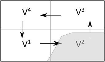
Figure 1. Schematic of the three-dimensional valley-plain system indicating the four control volumes and the mean along-valley circulation during the up-valley wind phase. The arrows indicate the net mass flux across the interfaces between adjacent control volumes. See Figure 3 for a top view of the valley-plain system.

2.1. Heat Budget and Advective Heat Transport

We first derive an expression for the net heat exchange of the valley with its surroundings due to advection. The bulk heat budget for an arbitrary control volume V can be expressed as

$\begin{array}{l}{\displaystyle \underset{m^i{\dot{\theta }}^i}{{\displaystyle \underbrace{{\displaystyle {\int }_V}\rho c_p\frac{\partial \theta }{\partial t}dV}}}}={\displaystyle \underset{F_{db}^i}{{\displaystyle \underbrace{{\displaystyle {\int }_{A_s}}{H}_{s}dS+{\displaystyle {\int }_V}\nabla ·RdV}}}}\\ +{\displaystyle \underset{F_a^i}{{\displaystyle \underbrace{{\displaystyle {\int }_V}\rho c_{p}v·\nabla \theta dV}}}}+{\displaystyle \underset{F_t^i}{{\displaystyle \underbrace{{\displaystyle {\int }_{A_a}}HdS}}}},& \left(1\right)\hfill \end{array}$

where H_s is the turbulent sensible heat flux normal to the land surface A_s, R is the radiation flux, and H is the turbulent sensible heat flux normal to the surface A_a. The surface A_a is the atmospheric component of the surface of the control volume V. For a conventional control volume the last term simplifies to the integral of the vertical turbulent sensible heat flux across the top surface of the control volume. Equation (1) is derived by integration of the potential-temperature equation and by using Gauss' theorem to convert the resulting volume integral of the turbulent heat flux divergence into a surface integral and by decomposing the resulting surface integral into a land surface part A_s and an atmospheric part A_a (as in Schmidli and Rotunno, 2010). In other words, the net change of heat content in an arbitrary volume Vⁱ ($m^i{\dot{\theta }}^i$) is equal to the sum of the contributions due to diabatic processes ($F_{db}^i$), mean-flow advection ($F_a^i$), and turbulent heat flux through A_a ($F_t^i$). Here mⁱ refers to the mass of the air in the volume Vⁱ, multiplied by the specific heat of the air, that is $m^i=c_p{\int }_{V^i}\rho \mathrm{ d}V$, and ${\dot{\theta }}^i$ refers to the density-weighted volume-averaged temperature tendency.

Now let us return to the valley-plain system, as illustrated in Figure 1. Our goal is to determine net heat exchange due to advection $F_a^2$ in the valley volume V². Assuming no diabatic heating and turbulent exchange in the upper plain volume V⁴, the bulk heat budgets for the four control volumes are

$\begin{array}{ll}{m}^1{\dot{\theta }}^1=F_{db}^1+F_a^1,\hfill & \left(2\right)\hfill \end{array}$

$\begin{array}{ll}{m}^2{\dot{\theta }}^2=F_{db}^2+F_a^2+F_t^2,\hfill & \left(3\right)\hfill \end{array}$

$\begin{array}{ll}{m}^3{\dot{\theta }}^3=F_{db}^3+F_a^3+F_t^3,\hfill & \left(4\right)\hfill \end{array}$

$\begin{array}{ll}{m}^4{\dot{\theta }}^4=F_a^4.\hfill & \left(5\right)\hfill \end{array}$

Assuming equal heating rates in the quasi-steady state, ${\dot{\theta }}^1={\dot{\theta }}^2$ and ${\dot{\theta }}^3={\dot{\theta }}^4$, and introducing

$\begin{array}{llll}{F}_{db}\equiv F_{db}^2,\hfill & F_a\equiv -F_a^2,\hfill & F_t\equiv -F_t^2,\hfill & \left(6\right)\hfill \end{array}$

$\begin{array}{lll}{\beta }_{db}\equiv F_{db}^3∕F_{db}^2,\hfill & {\beta }_a\equiv F_a^3∕F_a^2,\hfill & \left(7\right)\hfill \end{array}$

where the sign is chosen such that F_a ≥ 0 and F_t ≥ 0 during the daytime heating period, and noting that $F_t^3=-F_t^2$, the above equation system can be written as

$\begin{array}{ll}{m}^2(F_{db}^1+F_a^1)=m^1(F_{db}-F_a-F_t)\hfill & \left(8\right)\hfill \end{array}$

$\begin{array}{ll}{m}^4\left({\beta }_{db}{F}_{db}-{\beta }_a{F}_a+F_t\right)=m^3{F}_a^4.\hfill & \left(9\right)\hfill \end{array}$

Next, the net advective fluxes over the plain are related to those over the valley:

$\begin{array}{ll}{F}_a^1+F_a^4=(1+{\beta }_a)F_a+F_a^n,\hfill & \left(10\right)\hfill \end{array}$

where $F_a^n$ is the net advective exchange of the entire valley-plain system with its surroundings (later on we will assume that $F_a^n=0$). Solving (8) for $F_a^1$ and (9) for $F_a^4$ and substituting into (10) one obtains

$\begin{array}{l}\frac{m^1}{m^2}(F_{db}-F_a-F_t)-F_{db}^1+\frac{m^4}{m^3}({\beta }_{db}{F}_{db}-{\beta }_a{F}_a+F_t)\hfill \\ =(1+{\beta }_a)F_a+F_a^n.\hfill & \left(11\right)\hfill \end{array}$

Defining the mass (volume) ratios ${\tau }_{\upsilon }\equiv \frac{m^1}{m^2}$, ${\tau }_u\equiv \frac{m^4}{m^3}$, and the turbulent exchange ratio γ_t ≡ F_t∕F_db and factoring out F_a yields

$\begin{array}{l}{F}_a\left(1+{\beta }_a+{\tau }_{\upsilon }+{\tau }_u{\beta }_a\right)={\tau }_{\upsilon }(1-{\gamma }_t)F_{db}-F_{db}^1\hfill \\ +{\tau }_u({\beta }_{db}+{\gamma }_t)F_{db}-F_a^n.\hfill & \left(12\right)\hfill \end{array}$

Assuming equal diabatic forcing per unit area, the diabatic heat flux in the plain volume V¹ can be expressed by the diabatic heat flux in the valley volume by $F_{db}^1={\tau }_A{F}_{db}$, where τ_A is the ratio of the areas of the upper control surfaces of the plain and valley volume. [Under typical topographic amplification factor considerations (Whiteman, 1990), these surface areas would be assumed to be of equal size, hence τ_A = 1]. Substituting $F_{db}^1$ into (12) yields

$\begin{array}{ll}{f}_a\equiv \frac{F_a}{F_{db}}=\frac{{\tau }_{\upsilon }-{\tau }_A+{\beta }_{db}{\tau }_u-{\gamma }_t({\tau }_{\upsilon }-{\tau }_u)-{\delta }_a}{{\tau }_{\upsilon }+1+{\beta }_a({\tau }_u+1)},\hfill & \left(13\right)\hfill \end{array}$

where f_a represents the ratio of the advective to the diabatic forcing of the valley control volume and ${\delta }_a\equiv F_a^n∕F_{db}$ represents the net advective exchange of the entire valley-plain system with its surroundings. Note that (13) follows directly from the first law of thermodynamics and the three assumptions of quasi-steady state, equal diabatic forcing per unit area, and no diabatic or turbulent heating of the upper plain volume. It is valid for arbitary valley geometries. It can be seen that the advective heat flux increases if there is diabatic heating of the upper valley volume and it decreases if there is significant turbulent exchange. It also decreases if there is advective heating of the upper valley volume (i.e., β_a > 0). If one assumes that the valley-plain system is closed to external influences, i.e., negligible larger-scale flows, then δ_a = 0. Application of (13) requires diagnosis or estimation of the ratios β_db, γ_t, and β_a, and the geometric factors τ_υ, τ_A, and τ_u. In general, not all of these parameters are known a-priori.

As our goal is to derive scaling relations that can be applied a-priori, or with minimal additional assumptions, we assume that the flow-dependent parameters β_a and γ_t are approximately zero. In other words, assuming only diabatic heating of the upper valley volume, (13) reduces to

$\begin{array}{ll}{f}_a=\frac{{\tau }_h-1}{{\tau }_h+1∕{\tau }_A}+\frac{{\beta }_{db}{\tau }_u}{{\tau }_{\upsilon }+1},\hfill & \left(14\right)\hfill \end{array}$

where ${\tau }_h\equiv {\tau }_{\upsilon }∕{\tau }_A=h∕{\overline{h}}_{\upsilon }$ is the ratio of the mean depth of the plain to that of the valley control volume. For the standard case of equal upper control surfaces, τ_h corresponds to the topographic amplification factor (TAF). Returning to the heat budgets, it can be seen that in this limit, the diabatic heating of the upper valley volume is matched by a corresponding advective heating of the upper plain volume.

To provide further insight, suppose that β_db = 0 and that the surface areas of the valley and plain control volumes are identical, as is often done in TAF considerations (e.g., Whiteman, 1990), then τ_A = 1, and the advective heating ratio becomes

$\begin{array}{ll}{f}_a=\frac{{\tau }_h-1}{{\tau }_h+1}.\hfill & \left(15\right)\hfill \end{array}$

For illustration consider a valley with triangular cross section with τ_h = 2, then f_a = 1∕3 for the closed valley-plain system.

2.2. The Along-Valley Mass Flux

Using the advective ratio f_a, it is now possible to derive an a-priori estimate of the strength of the mean up-valley wind at the valley entrance. First note that the net advective heat flux out of the valley volume can be expressed as

$\begin{array}{ll}{F}_a=c_{p}M\Delta \theta ,\hfill & \left(16\right)\hfill \end{array}$

where M is the mass flux through the valley volume and Δθ = θ_out − θ_in is the difference in the mean potential temperature of the outflow and the inflow. Combining (16) and (13), the up-valley mass flux at the valley entrance is

$\begin{array}{ll}M=\frac{f_a{F}_{db}}{c_p\Delta \theta }=\frac{f_{db}}{c_p{c}_{\theta }{\gamma }_{\theta }}·\frac{LW}{h}·f_a,\hfill & \left(17\right)\hfill \end{array}$

where f_db is the diabatic heating rate per unit area, γ_θ is the potential temperature lapse rate, c_θ is an empirical constant relating the temperature difference Δθ to the lapse rate, L is the valley length, and W is the valley width.

Assuming that the inflow is through the valley entrance and the outflow is through the valley top, the mass flux is related to the mean along-valley wind through $M=\overline{v}\overline{\rho }{A}_{\text{in}}$. Substituting into (17), using (14) with β_db = 0, and rearranging, the mean up-valley wind at the valley entrance is

$\begin{array}{ll}\overline{\upsilon }=\frac{f_{db}}{c_p{c}_{\theta }{\gamma }_{\theta }h\overline{\rho }}·\frac{L}{{\overline{h}}_{\upsilon }}·\frac{{\tau }_h-1}{{\tau }_h+1∕{\tau }_A},\hfill & \left(18\right)\hfill \end{array}$

where $A_{\text{in}}=W{\overline{h}}_{\upsilon }$ has been used. It can be seen that the valley wind strength is proportional to the valley length, independent of the valley width, and inversely proportional to the square of the valley depth. It increases monotonically with increasing TAF (τ_h).

2.3. Parameter Estimation

Several parameters are required in order to estimate the up-valley mass flux using (17) and the advective heating ratio using (14). Some of these parameters, such as τ_h, β_db, and τ_υ, depend on the choice of the control volumes, in particular on the height h of the upper control surfaces of the valley and plain volume. They can be calculated directly from the given topography as a function of the height h, once the horizontal location of the control volumes has been fixed, as illustrated in Figure 2. It can be seen that the TAF, τ_h, increases with decreasing height of the control volume, as has been pointed out by Steinacker (1984). If h is smaller than the crest height h_c, the diabatic ratio β_db becomes non-zero and increases with decreasing h. Assuming uniform diabatic forcing per unit area, β_db is equal to the area fraction occupied by topography on the lower surface of the upper control volume (for h > h_c, this area fraction is zero).

FIGURE 2

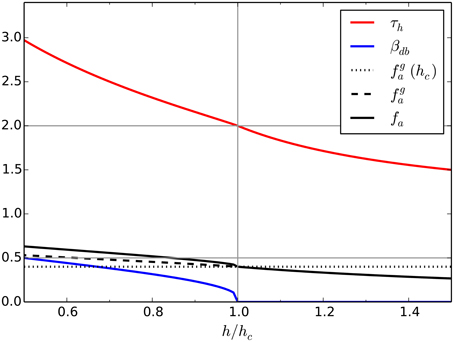
Figure 2. Dependence of the parameters τ_h, β_db and the different approximations of the advective ratio f_a (see main text) on the height of the upper control surface (depth of the control volume), for the topography to be introduced in Section 3 and illustrated in Figure 3.

Two choices for estimating the parameters are considered: first, h equal to the height of the mountain crest, h_c; second, h equal to the height of the “equilibrium” level, h_e, that is the level of zero mean along-valley flow. The first choice corresponds to the standard application of the TAF argument; all required parameters, except c_θ, can be calculated a-priori. The second choice better represents the true flow geometry, in particular the depth of the up-valley flow layer. If h_e is known, then the required parameters can be calculated.

As we are interested in the a-priori scaling of the valley wind, a simplified estimate of the advective ratio is introduced. Assuming that β_db ≈ 0, one obtains

$\begin{array}{ll}{f}_a^g=\frac{{\tau }_h-1}{{\tau }_h+1∕{\tau }_A}\hfill & \left(19\right)\hfill \end{array}$

It can be seen that $f_a^g$ depends only on parameters related to the valley geometry and can thus be calculated a-priori, if h is given.

In summary, three different approximations of the up-valley mass flux and the advective heating ratio will be compared in comparison to the numerical simulations to be introduced next. The simplest approximation is based on the parameters evaluated with h = h_c. The next is based on (19) using h = h_e, and the final, and potentially most accurate estimate, is based on (14) and also using h = h_e. For the latter β_db > 0 if h_e < h_c.

3. Numerical Setup

The numerical setup of the simulations is similar to the one described in Schmidli and Rotunno (2010, 2012) (hereafter SR10 and SR12) and detailed information can be found there. For convenience we summarize the main aspects of the setup and point out the key differences with respect to SR10. To investigate the quasi-steady state of the valley wind system, we introduce a valley-plain configuration with a horizontal valley floor as shown in Figure 3. Except for the east-west orientation, the topography is identical to the periodic configuration introduced in SR12, and the corresponding analytic expression for the topography can be found in SR12. To save computing resources, the cross-valley extension of the computational domain is reduced from 120 to 20 km. For the periodic configuration this does not influence the results.

FIGURE 3

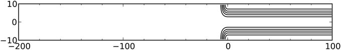
Figure 3. Computational domain adopted in this paper. The lines denote the height contours of the topography (contour interval = 250 m).

As in SR10, the simulations are initialized from an atmosphere at rest with a constant stratification. The main difference with respect to SR10 is in the thermal forcing of the valley wind system. As we are interested in the quasi-steady state, the wind system is forced by a constant surface sensible heat flux. In contrast to the previous simulations, the land surface model is turned off. Momentum transfer is determined by a constant momentum drag coefficient, corresponding to a neutral surface layer and a given momentum roughness length. While the simulations are integrated for 14 h, our main focus is on the scaling properties after 9 h, when the simulation is close to a steady-state.

To investigate the scaling of the quasi-steady state, a set of simulations are carried out. The set is created by varying the valley dimensions, the lapse rate of the initial state, the thermal forcing in terms of the prescribed surface sensible heat flux, and the momentum roughness length. The reference simulation comprises a valley with a length of 100 km, a crest-to-crest width of 20 km, and a depth of 1500 m, a potential temperature lapse rate of +3 K km⁻¹, a surface sensible heat flux of 50 W m⁻², and a momentum roughness length of 0.1 m. All experiments are created by varying one parameter in comparison to the reference simulation (see Table 1).

TABLE 1

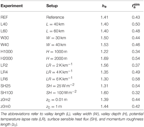
Table 1. Summary of the numerical experiments.

As in SR10, the numerical simulations have been carried out using the Advanced Regional Prediction System (ARPS) model (Xue et al., 2000, 2001). The horizontal grid spacing is 1 km and the vertical grid spacing varies from 20 m near the surface to a maximum of 200 m above 2 km. The lateral boundary conditions are periodic in the cross-valley direction and free-slip wall conditions are imposed in the along-valley direction. This choice minimizes the required computational resources, as doubly periodic boundary conditions would require a computational domain of double the current size in the along-valley direction. In order to reduce the implicit diffusivity of the integration, horizontal and vertical advection of momentum and scalars is carried out by a 4th-order advection scheme (in SR10, vertical advection is carried out by a 2nd-order scheme). Thus, the time step had to be reduced from 12 to 6 s. Vertical mixing is parameterized with a TKE-based PBL scheme using a non-local turbulence length scale (Sun and Chang, 1986). All moist processes are turned off (moist=0). The current setup was chosen in order to be able to do many simulations. Although large-eddy simulations for two-dimensional valley sections are now fairly common (e.g., Catalano and Moeng, 2010; Serafin and Zardi, 2010; Schmidli, 2013; Wagner et al., 2014), and even isolated examples of large-domain simulations of the along-valley wind exist (Schmidli, 2013; Wagner et al., 2015a,b), for the purpose of the present study simulations using parameterized turbulence are sufficient. We have found that for well-resolved valleys mean and bulk quantities obtained with the current setup compare well with large-eddy simulation results (see also Wagner et al., 2014).

4. Results

Next, we test the formula for the advective heating ratios and the along-valley mass flux for the set of numerical simulations introduced above. The section starts with a brief discussion of the evolution of the reference simulation, followed by the presentation of the main results on the net advective heat flux (heat export out of the valley control volume) and the along-valley mass flux.

4.1. The Reference Simulation

Snapshots of the evolution of the valley wind system are shown in Figure 4 after 3, 6, and 9 h of integration. The figure illustrates the evolution of the along-valley flow, both in an along-valley plane located at the valley center and in a cross-valley plane located 20 km up valley from the valley entrance, the cross-valley circulation and the thermal structure of the atmosphere. The basic characteristics of the flow are very similar to previous simulations with a time-dependent diurnal forcing. The symmetric cross-valley circulations develop rapidly, while the along-valley circulation takes longer to develop fully. It can be seen that while the up-valley component of the along-valley circulation (on the valley center plane) is already close to a steady state after 6 h, the upper-level return flow is still increasing between hours 6 and 9. Note also the suppression of the growth of the convective boundary layer within the valley, which is clearly visible in the along-valley sections. For a more detailed discussion of the evolution of the valley wind system, see SR10 and SR12. As already noted in SR12, the disturbances in the along-valley flow pattern near the valley entrance seen after 9 h are likely related to the ARPS turbulence scheme and unresolved cellular motions in the convective boundary layer (Ching et al., 2014). Other models do not show such quasi-periodic patterns (Schmidli et al., 2011). Toward the end of the simulation these patterns may dominate the flow. Luckily they do not significantly influence the early stages of the quasi-steady state which is the focus of our study.

FIGURE 4

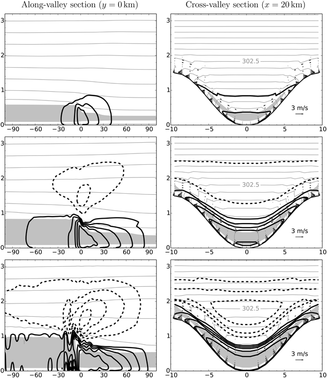
Figure 4. Evolution of the valley wind system for the reference case. Along-valley and cross-valley sections after 3, 6, and 9 h of integration showing the along-valley flow (thick contours; contour interval = 0.5 m s⁻¹; negative values are dashed), potential temperature [contour interval = 1 K (left panels) and 0.5 K (right panels)], eddy diffusivity (shading; 10 m² s⁻¹), and the cross-valley circulation (wind vectors). The axis units are kilometers.

The approach to the quasi-steady state is depicted in Figure 5 in terms of the evolution of the mean up-valley wind (at the valley entrance) and the valley heat budget. During the first 6 h, the mean along-valley wind increases approximately linearly. Thereafter, as the valley wind system approaches the quasi-steady state, the increase is much reduced and the mean along-valley wind reaches its maximum value of about 2.2 m s⁻¹ after 10 h. In terms of the heat budget, and in particular the net advective heat flux, the components are already steady after 6–7 h. The simulated cooling rate due to advection is close to the a-priori estimate indicated by the dashed line. Note that the net heat exchange due to turbulence is close to zero for the reference simulation. This is due to the combination of a relatively deep valley, sufficient stratification and relatively weak surface forcing. It can be seen that after 10 h of integration there are deviations from the steady-state values. This is due to the ARPS-specific disturbances discussed above. In order to avoid issues related to these disturbances we will focus on hour 9 for the analysis of the quasi-steady state.

FIGURE 5

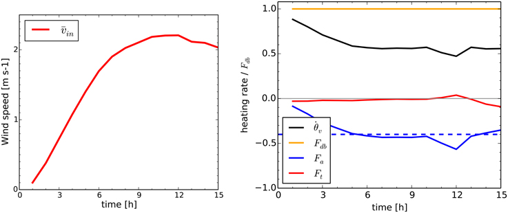
Figure 5. Time evolution of the mean up-valley wind at the valley entrance (left panel) and the heat budget tendencies for the valley control volume (right panel). ${\overline{\upsilon }}_{in}$ denotes the average of the along-valley wind over the inflow layer, that is up to h_e. The dashed line indicates the a-priori estimate, f_a(h_c), of the steady-state advective heating rate.

4.2. Net Advective Heat Flux

The quasi-steady state predictions of the net advective heat flux out of the valley control volume are compared with the diagnosed value from the numerical simulations in Figure 6. The scaling predictions correspond to the three approximations introduced in Section 2.3. The most basic approximation corresponds to the assumption that the top of the valley control volume corresponds to the height of the mountain ridges [i.e., f_a = f_a(h_c)]. While this assumption results in reasonable estimates for some of the valleys, it fails to represent the variations associated with changes in the valley depth, the atmospheric stratification, and the surface sensible heat flux. Further analysis shows that this failure is partly related to the varying depth of the up-valley wind layer. For the simulation with strong stability, for example, the up-valley wind layer is restricted to a depth of less than 1 km and the upper-level return flow occurs already at heights well below the mountain ridge height (not shown).

FIGURE 6

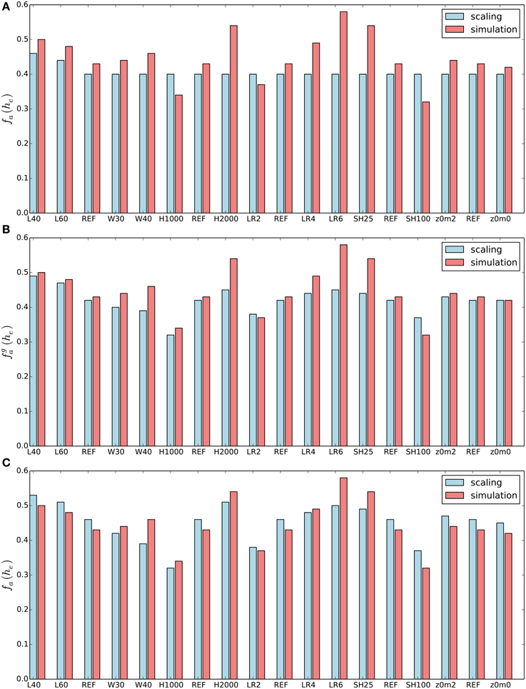
Figure 6. Scaling the advective heat flux: comparison of different approximations of f_a with the diagnosed value from the numerical simulations. (A) basic approximation: f_a = f_a(h_c), (B) improved estimate with $f_a=f_a^g(h_e)$, (C) improved estimate with f_a = f_a(h_e).

In order to improve the estimate of f_a, the true flow geometry needs to be considered. From the cross-valley averaged along-valley circulation at the valley entrance, one can estimate the height of the mean inflow, the mean outflow, and the level of zero net along-valley flow. For the reference simulation the zero-flow height corresponds to 1.41 km. The results for the other simulations are tabulated in Table 1 and visualized in Figure 7. Improved estimates of f_a can now be obtained by setting the top of the lower control volumes to the zero-flow height. These are denoted by $f_a^g(h_e)$ and f_a(h_e). The former represents only the more accurate consideration of the flow geometry, while the latter also includes the effect of a non-zero diabatic factor β_db. Consideration of the flow geometry leads to an overall improvement of the estimates. The correspondance between the analytic estimates and the diagnosed values from the numerical simulations is further increased by including the effect of the non-zero diabatic factor, except for the simulations with different valley widths. Much of the remaining differences (e.g., for LR6, SH25) are likely due to larger deviations from the quasi-steady-state assumption for the particular simulations (not shown).

FIGURE 7

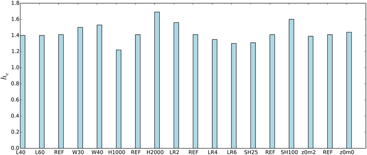
Figure 7. Diagnosed depth of the inflow layer, h_e.

In summary, the a-priori estimation of the net advective heat flux out of the valley volume is successful if the zero-flow height is close to the valley ridge height, or if the corresponding zero-flow height can be estimated (a-priori), provided the circulation is approximately in a quasi-steady state.

4.3. The Along-Valley Mass Flux

Once the net advective heat flux out of the valley control volume is known, it is possible to estimate the along-valley mass flux and thus the strength of the mean along-valley wind at the valley entrance. The key idea is that the net advective heat flux is proportional to the mass flux through the valley control volume and the difference in the mean potential temperature of the mean inflow into the valley volume and the mean outflow out of the valley volume, see (16).

The scaling of the along-valley mass flux according to the (a-priori) quasi-steady state estimates and the numerical simulations is depicted in Figure 8, for the same three approximations discussed above. Note that both the estimated and the diagnosed values are scaled with respect to the reference case, i.e., REF = 1. Even for the most basic approximation, M(h_c), the scaling of the along-valley mass flux works quite well. Larger differences are only found for H1000, LR2, and SH100, the three cases for which the inflow layer extends above the crest height (i.e., h_e > h_c, see Table 1). This indicates that the a-priori scaling is less accurate if the valley is shallow in comparison to the surface forcing and the stratification. If the valley is too shallow, that is if the convective boundary layer extends well beyond the crest height, the scaling does not work (additional simulations with shallower valleys were undertaken, but are not shown).

FIGURE 8

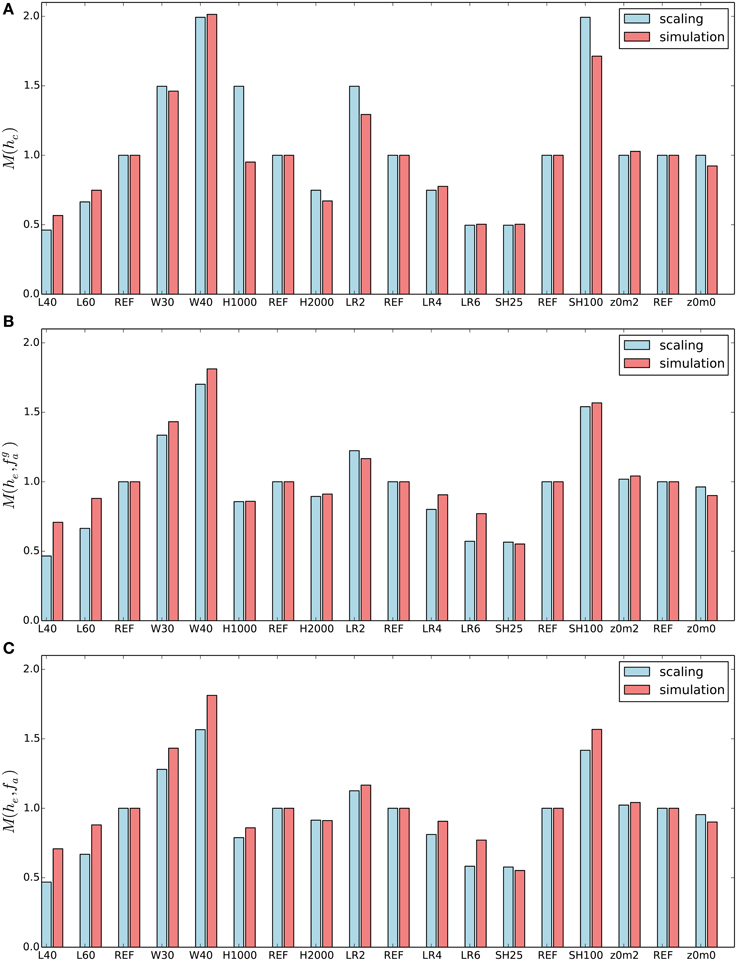
Figure 8. Scaling the along-valley mass flux M: comparison of different a-priori estimates of M with the corresponding diagnosed value from the numerical simulations. (A) Basic approximation M = M(h_c), (B) improved estimate with $M=M(h_e,f_a^g)$, (C) improved estimate with M = M(h_e, f_a). The former estimate is compared to the simulated along-valley flux up to ridge height, the latter two estimates are compared to the total simulated up-valley flux, that is to the height h_e.

The lower two panels show the scaling of the up-valley mass flux, that is of the along-valley mass flux up to the equilibrium height h_e, for the two approximations of f_a. Overall the performance of the scaling is quite similar for both cases, with a slightly higher overall skill for the simpler estimate $f_a^g$. Comparing the simpler estimate (middle panel) with the a-priori scaling (top panel), the skill is clearly improved for variations of the valley depth and of the surface sensible heat flux.

According to the analysis presented in Section 2, the steady-state along-valley wind and the associated mass and heat fluxes should be independent of the surface roughness (friction). Comparing the three simulations with different surface roughnesses (0.01, 0.1, and 1.0 m), it is found that this is indeed approximately the case. The pressure gradient forcing adjusts itself in order to support roughly the same along-valley mass flux. Note that the near-surface wind speed is of course reduced for large roughness lengths, but this has only a minor effect on the integrated along-valley mass flux (not shown).

In summary, the scaling of the along-valley mass flux (and hence of the along-valley wind) with respect to variations of the valley geometry, atmospheric stratification, and surface sensible heat flux is successful, provided the up-valley wind circulation (and hence the convective boundary layer) does not extend significantly above the height of the surrounding mountain ridges. This implies that the valleys need to be sufficiently deep, given the specific combination of surface forcing and atmospheric stratification.

5. Conclusions

The quasi-steady-state limit of the diurnal valley wind system has been examined in order to contribute to an improved understanding of the along-valley winds and the associated transport processes. A scaling relation for the steady-state along-valley wind speed and the associated advective heat flux as a function of valley geometry, valley size, atmospheric stratification, and surface sensible heat flux forcing has been derived. In contrast to results from simple dynamical models (e.g., Vergeiner, 1987), the steady-state scaling is also valid for complex valley geometries. The formula can be used as a diagnostic tool or for the a-priori estimation of the along-valley mass flux and the valley-wind strength in a given situation. The a-priori estimation requires either additional closure assumptions or the use of an approximate formula.

It is found that the steady-state along-valley wind speed increases linearly with the magnitude of the surface forcing and the strength of the valley volume effect (τ_h−1), these two factors correspond to the extra heating factor in simple linear models (Egger, 1990). Also as in the linear case, the wind speed decreases with increasing atmospheric stability. In contrast to the results from simple dynamical models, the steady-state wind speed increases with increasing valley length and it is largely independent of the surface roughness. This may at first seem counterintuitive, but can easily be understood. The initial evolution of the along-valley wind is of course restrained by surface friction, but in the steady state the plain-temperature contrast will increase until the along-valley pressure gradient is strong enough to support the along-valley wind required by the steady-state valley heat budget. Also the longer valley, the larger the excess heat that needs to be exported out of the valley to maintain a steady-state heat budget. In summary, the strength of the steady-state valley wind is primarily controlled by the diabatic forcing and the atmospheric stability, and not by surface friction. This scaling prediction is confirmed by the numerical simulations.

The scaling relation for the steady-state mass and heat flux is tested by comparison with the corresponding diagnosed fluxes from numerical simulations of the along-valley wind system for idealized three-dimensional topographies. In general, good agreement is found. The scaling of the along-valley mass flux with respect to variations of the valley geometry, atmospheric stratification, and surface sensible heat flux works well, provided the valley is sufficiently deep, such that the convective boundary layer (and hence the up-valley flow layer) does not extend significantly above the height of the surrounding mountain ridges.

The quasi-steady state scaling relations can be used for the a-priori estimation of the mass and heat fluxes associated with the along-valley circulation. Two different approximations of the scaling relations have been developed and tested. The first one assumes that the budgeting volumes extend to the top of the mountain ridge; the second one sets the height of the budgeting volumes to the top of the inflow layer. While the former approximation can be calculated a-priori, the latter requires the height of the inflow layer as an input. The results show that this height is strongly correlated with variations of the valley depth and the atmospheric stratification. This opens up the possibility for the development of a parameterization of the depth of the inflow layer and thus of using also the more complete scaling relations in an a-priori setup. This requires further investigation. In any event it points to the most important parameter dependencies for estimating the along-valley mass flux. The a-priori scaling relations could be used as a basis to parameterize the larger-scale effects of the thermally-induced along-valley circulations in coarse-resolution weather and climate models.

Conflict of Interest Statement

The authors declare that the research was conducted in the absence of any commercial or financial relationships that could be construed as a potential conflict of interest.

Acknowledgments

The numerical simulations have been performed on the CRAY XE6 at the Swiss National Supercomputing Centre (CSCS) using the Advanced Regional Prediction System (ARPS) developed by the Center for Analysis and Prediction of Storms, University of Oklahoma. The figures have been produced using matplotlib (Hunter, 2007).

References

Banta, R. M. (1990). “The role of mountain flows in making clouds,” in Atmospheric Processes Over Complex Terrain, Meteorological Monographs, Vol. 23, ed W. Blumen (Boston, MA: American Meteorological Society), 229–283.

Catalano, F., and Moeng, C.-H. (2010). Large-eddy simulation of the daytime boundary layer in an idealized valley using the weather research and forecasting numerical model. Bound. Layer Meteorol. 137, 49–75. doi: 10.1007/s10546-010-9518-8

CrossRef Full Text | Google Scholar

Ching, J., Rotunno, R., LeMone, M., Martilli, A., Kosovic, B., Jimenez, P. A., et al. (2014). Convectively induced secondary circulations in fine-grid mesoscale numerical weather prediction models. Mon. Weather Rev. 142, 3284–3302. doi: 10.1175/MWR-D-13-00318.1

CrossRef Full Text | Google Scholar

Egger, J. (1987). Simple models of the valley-plain circulation. Part I: minimum resolution model. Meteorol. Atmos. Phys. 36, 231–242. doi: 10.1007/BF01045151

CrossRef Full Text | Google Scholar

Egger, J. (1990). “Thermally forced flows: theory,” in Atmospheric Processes Over Complex Terrain, Meteorological Monographsm, Vol. 23, ed W. Blumen (Boston, MA: American Meteorological Society), 43–58.

Hunter, J. D. (2007). Matplotlib: a 2D graphics environment. Comput. Sci. Eng. 9, 90–95. doi: 10.1109/MCSE.2007.55

CrossRef Full Text | Google Scholar

Rampanelli, G., Zardi, D., and Rotunno, R. (2004). Mechanisms of up-valley winds. J. Atmos. Sci. 61, 3097–3111. doi: 10.1175/JAS-3354.1

CrossRef Full Text | Google Scholar

Schmidli, J. (2013). Daytime heat transfer processes over mountainous terrain. J. Atmos. Sci. 70, 4041–4066. doi: 10.1175/JAS-D-13-083.1

CrossRef Full Text | Google Scholar

Schmidli, J., Billings, B., Chow, F. K., De Wekker, S. F. J., Doyle, J., Grubisic, V., et al. (2011). Intercomparison of mesoscale model simulations of the daytime valley wind system. Mon. Weather Rev. 139, 1389–1409. doi: 10.1175/2010MWR3523.1

CrossRef Full Text | Google Scholar

Schmidli, J., and Rotunno, R. (2010). Mechanisms of along-valley winds and heat exchange over mountainous terrain. J. Atmos. Sci. 67, 3033–3047. doi: 10.1175/2010JAS3473.1

CrossRef Full Text | Google Scholar

Schmidli, J., and Rotunno, R. (2012). Influence of the valley surroundings on valley-wind dynamics. J. Atmos. Sci. 69, 561–577. doi: 10.1175/JAS-D-11-0129.1

CrossRef Full Text | Google Scholar

Serafin, S., and Zardi, D. (2010). Daytime heat transfer processes related to slope flows and turbulent convection in an idealized mountain valley. J. Atmos. Sci. 67, 3739–3756. doi: 10.1175/2010JAS3428.1

CrossRef Full Text | Google Scholar

Steinacker, R. (1984). Area-height distribution of a valley and its relation to the valley wind. Contrib. Atmos. Phys. 57, 64–71.

Google Scholar

Sun, W.-Y., and Chang, C.-Z. (1986). Diffusion model for a convective layer. Part I: numerical simulation of convective boundary layer. J. Clim. Appl. Meteorol. 25, 1445–1453. doi: 10.1175/1520-0450(1986)025<1445:DMFACL>2.0.CO;2

CrossRef Full Text | Google Scholar

Vergeiner, I. (1987). An elementary valley wind model. Meteorol. Atmos. Phys. 36, 264–286. doi: 10.1007/BF01045154

CrossRef Full Text | Google Scholar

Vergeiner, I., and Dreiseitl, E. (1987). Valley winds and slope winds — observations and elementary thoughts. Meteorol. Atmos. Phys. 36, 264–286. doi: 10.1007/BF01045154

CrossRef Full Text | Google Scholar

Wagner, A. (1938). Theorie und beobachtung der periodischen gebirgswinde. Gerlands Beitr. Geophys. 52, 408–449.

Wagner, J. S., Gohm, A., and Rotach, M. W. (2014). Impact of horizontal model grid resolution on the boundary layer structure over an idealized valley. Mon. Weather Rev. 142, 3446–3465. doi: 10.1175/MWR-D-14-00002.1

CrossRef Full Text | Google Scholar

Wagner, J. S., Gohm, A., and Rotach, M. W. (2015a). The impact of valley geometry on daytime thermally driven flows and vertical transport processes. Q. J. R. Meteorol. Soc. 141, 1780–1794. doi: 10.1002/qj.2481

CrossRef Full Text | Google Scholar

Wagner, J. S., Gohm, A., and Rotach, M. W. (2015b). Influence of along-valley terrain heterogeneity on exchange processes over idealized valleys. Atmos. Chem. Phys. 15, 6589–6603. doi: 10.5194/acp-15-6589-2015

CrossRef Full Text | Google Scholar

Whiteman, C. D. (1990). “Observations of thermally developed wind systems in mountainous terrain,” in Atmospheric Processes over Complex Terrain, Meteorological Monographs, Vol. 23, ed W. Blumen (Boston, MA: American Meteorological Society), 5–42.

Wyngaard, J. C. (2010). Turbulence in the Atmosphere. Cambridge: Cambridge University Press.

Google Scholar

Xue, M., Droegemeier, K. K., and Wong, V. (2000). The advanced regional prediction system (ARPS)—A multi-scale non-hydrostatic atmospheric simulation and prediction model. Part I: Model dynamics and verification. Meteor. Atmos. Phys. 75, 161–193. doi: 10.1007/s007030070003

CrossRef Full Text | Google Scholar

Xue, M., Droegemeier, K. K., Wong, V., Shapiro, A., Brewster, K., Carr, F., et al. (2001). The advanced regional prediction system (ARPS)—A multi-scale nonhydrostatic atmospheric simulation and prediction model. Part II: Model physics and applications. Meteor. Atmos. Phys. 76, 143–165. doi: 10.1007/s007030170027

CrossRef Full Text | Google Scholar

Zardi, D., and Whiteman, C. D. (2013). “Observations of thermally developed wind systems in mountainous terrain,” in Mountain Weather Research and Forecasting – Recent Progress and Current Challenges, Springer Atmospheric Sciences, eds F. K. Chow, S. F. J. DeWekker, and B. Snyder (Berlin: Springer), 35–122.