High-Accuracy Elevation Data at Large Scales from Airborne Single-Pass SAR Interferometry

1. Introduction

Elevation data in the form of a digital elevation model (DEM) are probably the most common remote sensing-derived product and are required for most types of environmental applications; however height accuracies vary greatly with technology and spatial resolution. For some applications high vertical precision and accuracy may be less important (e.g., large-scale hydrologic modeling) but mapping heights accurately is required for applications that look at dynamic processes over subtle variations in topography, such as mapping and modeling floodplain inundation. Table 1 provides a detailed overview and commonly reported accuracies of the different DEMs that exist.

TABLE 1

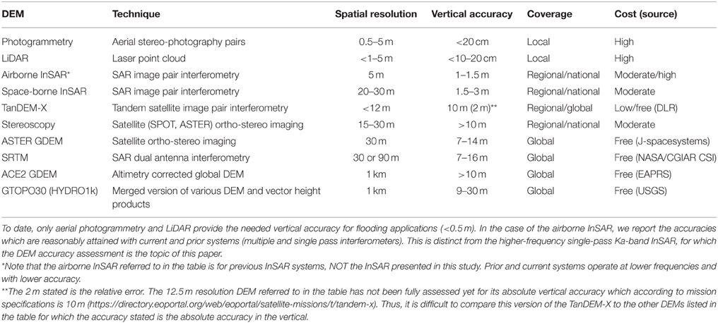
Table 1. Sources of common digital elevation models, with spatial resolutions and typical vertical accuracies as compiled from literature and mission specifications.

Fifteen years ago airborne laser altimetry or LiDAR allowed the creation of high spatial resolution (1–5 m) and accuracy (vertical error < 20 cm) DEMs that have transformed flood modeling and forecasting at regional to national scales in many developed countries (Bates, 2004). However, at continental or global scales the best currently available DEMs come from satellite acquisitions (Table 1) that do not meet even basic requirements for simulating flooding and related risks (health, wetland ecology and biodiversity, inundation residence times with important implications for bio-geochemical cycling). Globally available DEMs have vertical errors of 10 m or more and do not resolve the detail of terrain features that control flooding (Sanders, 2007).

It is clear that global coverage DEMs with low vertical accuracies may not be useful for local scale detailed floodplain inundation studies. However, in some low-lying floodplain areas, the SRTM-DEM at 90 m resolution for instance has been shown to be accurate to better than 2 m in the vertical (Schumann et al., 2013). Since flooding occurs mostly in those area, many of the global coverage DEMs (e.g., SRTM-DEM) may be used for large scale flood inundation studies although high accuracy (model) results can only really be obtained with airborne LiDAR DEM at local to regional scales. It is noteworthy though that recent advances in hydrodynamic modeling are moving toward improved representation of physics in models that can credibly simulate flood processes at sub-grid scale using coarse resolution and lower accuracy DEMs [e.g., LISFLOOD-FP sub-grid channel (SGC) as developed by Neal et al., 2012].

Nonetheless, the ideal situation would be to have a global and freely accessible DEM with LiDAR-like resolution and accuracies, and whilst the technology to create a high-resolution, high accuracy global DEM using fine resolution satellite stereo images has existed for some time, at present there is no international plan to develop such a product. Now with recent advances in flood modeling and supercomputing, and the increasing abundance of high resolution stereo imagery, we believe that it is time to open negotiations to free up the necessary financial support to achieve this, possibly from a consortium of industry, governments and humanitarian agencies. With annual losses due to flooding of US $1 trillion predicted by 2050 (Hallegatte et al., 2013), producing such a DEM at the global scale would be the environmental equivalent of the Human Genome Project (HGP; NIH, 2010). In 1990, the National Institutes of Health (NIH) and the US Department of Energy joined with international partners in a massive and costly undertaking to sequence the entire human genome and make data publicly available over the Internet, which would allow developing the tools to fight cancer and other genetic diseases. This concerted, public effort was the Human Genome Project and was completed under budget and 2 years ahead of schedule 23 years later for a total cost of US $2.7 billion (FY 1991 dollars), which is now largely outweighed by the advances made in biotechnology, genetic testing and treatment of genetic diseases. Similarly, having a global high resolution and high accuracy DEM would have enormous impacts on finance (e.g., flood re-insurance), humanitarian services (disaster relief services, disease prevention, etc.) and scientific research. Schumann et al. (2014) argue that this could be achieved for a cost of perhaps a few hundred million dollars using existing LiDAR data, stereo satellite photogrammetry and acquisition of new LiDAR elevation data either on board aircraft already operated for disaster relief operations or on drones deployed over floodplains. This is significantly cheaper than most satellite missions, yet would be transformative across a huge range of fields.

Although LiDAR-DEMs are of very high spatial resolution and great vertical accuracy (typical error: < 0.2 m) acquisition operations can be very costly for spatial scales larger than a couple of 100 square km and also have severe limitations in wetland areas and under cloudy and rainy conditions. Ideally, a DEM technology is needed that allows larger spatial coverage than LiDAR but without compromising resolution and vertical accuracy and still performing under some adverse weather conditions and at a reasonable cost. In some countries, DEMs at a fine spatial resolution and with a typical vertical error of around 1 m have been acquired at national level using airborne Interferometric Synthetic Aperture Radar (InSAR), requiring however multiple offset observations to generate the DEM. Radar interferometry holds a unique promise here, but typically has suffered from vertical errors which exceed requirements for flood-modeling needs (better than 0.5 m accuracy in the vertical), and uncertainty with respect to penetration of the electromagnetic wave in to the surface media. However, the GLISTIN-A (Glacier and Interferometric Ice Surface Topography Interferometer-Airborne) NASA airborne mission offers a novel single pass In-SAR technology that can efficiently generate DEMs over significant regions with a vertical precision of ranging from 0.3 m in the near range to 3 m in the far range at a spatial resolution of 3 m (Moller et al., 2011). With appropriate calibration, the Ka-band system enables high-accuracy high-resolution wide-swath mapping with minimal surface penetration as a potentially cost effective solution.

To demonstrate this capability (high resolution, cost-effective floodplain and flood hazard mapping), we compare a sample single-pass In-SAR Ka-band DEM of the California Central Valley from the NASA/JPL airborne GLISTIN-A mission to a very high-resolution LiDAR DEM as well as the Shuttle Radar Topography Mission (SRTM) DEM at 30 m. We also perform a simple sensitivity analysis to flood inundation.

2. Materials and Methods

2.1. SAR Data Generation and Calibration

GLISTIN-A is a Ka-Band (8 mm wavelength) cross-track single-pass InSAR, developed for high-precision, high-resolution ice-surface topography mapping over a swath of a width of about 10 km. The short wavelength minimizes penetration of the electromagnetic wave into the surface media and hence prevents any significant volume scattering from entering into the measured echoes, a great advantage, as this removes a major difficulty in interpreting the backscattering echoes. Airborne laser altimetry is similarly unaffected by any unwanted volume returns, but it is limited in swath width (up to 500 m) and hence in spatial coverage. As a quick reference, Table 2 shows a fair comparison of the main characteristics between standard LiDAR and the InSAR system presented here.

TABLE 2

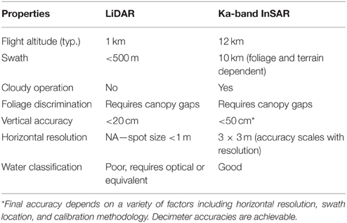
Table 2. Comparing LiDAR and Ka-band InSAR.

InSAR is able to retrieve surface topography by displacing two antennas in the cross-track direction to view the same surface. The interferometric combination of data received on the two antennas allows one to resolve the path-length difference from the illuminated area to a fraction of a wavelength. From the interferometric phase the height of the target (or phase center) can be estimated. Therefore, an InSAR system such as GLISTIN-A is capable of providing not only the position of each image point in along-track and slant range as with a traditional SAR, but also the height of that point through the use of the interferometric phase (Rodriguez and Martin, 1992; Rosen et al., 2000).

For the InSAR DEM, there is inherently a trade-off between spatial resolution and relative vertical accuracy in the final product. That is with spatial averaging the vertical precision of the final product can be improved at the expense of resolution (Rodriguez and Martin, 1992). In this paper we exploit this property to produce a lower resolution (30 × 30 m) from the original 3 × 3 m gridded product to reduce the random errors on the DEM product to an acceptable level for a variety of applications such as flood inundation modeling. In addition to averaging to reduce the level of the random errors, the swath data must also be calibrated due to systematic tilts across the GLISTIN-A height maps. These are the result of imperfect platform attitude knowledge and residual calibration errors not captured within the instrument calibration loop. Although these residuals are small, the bias effect can be large (up to a few meters) at the far-look angles where the imperfect knowledge is effectively multiplied by the cross-track distance. Fortunately, this effective ramp can be relatively straightforward to correct by estimating the bias in the far range and providing a linear correction. Several approaches and sources can be used to determine the correction:

• overlapping near-range of one swath with far-range of another,

• using ground-control points if available,

• using LiDAR altimetry if available (spaceborne or airborne).

In this paper we use the a priori airborne LiDAR data to estimate the cross-track systematic we apply to the InSAR swath data as described subsequently. The LIDAR data were collected in winter 2008 and the radar data in February, 2013 resulting in some difficulty in direct comparison due to some seasonal and time difference. In particular crops were likely at different heights. However, by carefully identifying relatively static regions a robust calibration can be derived.

2.2. SAR DEM Generation

As outlined in the previous section, the swath data must be calibrated due to systematic tilts across the GLISTIN-A height data. In our case, we were working with data that had not been fully calibrated, and as such the range-tilt accounted for 4.9 m at 13 km across track. A linear slope correction perpendicular to flight path was thus performed using the LiDAR height data set as a reference approximately two-thirds across the swath. Subsequently, a low-pass moving average filter was applied in a 5 × 5 window to attenuate the random noise.

In addition to accounting for SAR-specific effects, natural floodplains are often vegetated to various degrees of densities and with different vegetation heights and types, thus making it challenging to determine accurate bare ground elevation desirable for a variety of applications, in particular flow modeling. Although for LiDAR data, automated algorithms to remove Earth surface features are routinely and successfully applied (e.g., Cobby et al., 2001, 2003), SAR height data prove far more challenging given the inherent errors in the data and only limited progress has been achieved over recent years, often using ancillary data sets or models (e.g., Baugh et al., 2013).

However, the high-resolution and precision of these data we believe will allow for more robust classification schemes which in turn will enable bare-Earth DEM generation for many floodplain regions, with the exception of densely vegetated regions. In this instance we classified vegetated areas from the InSAR height precision data (Figure 2B). The height precision, σ_h, is derived from the measured interferometric correlation, γ, via the relation:

$\begin{array}{cc}\begin{array}{l}{\sigma }_h=\frac{\partial h}{\partial \varphi }{\sigma }_{\varphi }=\frac{\partial h}{\partial \varphi }\frac{1}{\sqrt{2N_L}}\sqrt{\frac{1-{\gamma }^2}{{\gamma }^2}}\\ \approx \frac{\lambda x}{4\pi B_{\perp }}\frac{1}{\sqrt{2N_L}}\sqrt{\frac{1-{\gamma }^2}{{\gamma }^2}},\end{array}& \left(1\right)\end{array}$

where λ is the electromagnetic wavelength, ϕ is the interferometric phase, x is the cross-track distance, B_⊥ is the projection of the interferometric baseline (vector separation between the antennas) onto the direction perpendicular to the look direction, and N_L is the number of independent pixels averaged to produce an elevation post. Note that σ_h is directly proportional to the cross-track distance. Over vegetation, increased volume scattering results in a lower correlation and thus an increased height error as observed in Figure 2B. We also observed that these regions were relatively bright and thus we coupled the InSAR relative backscattered power with the height precision to classify vegetated fields. After identifying the regions, we employed an iterative process to remove vegetation and other surface objects which considers first order height statistics of neighboring near-ground areas.

2.3. Demonstration Site

The demonstration site we chose from the GLISTIN-A flight path over the California Central Valley is a 30 km section of the San Joaquin River upstream of the city of Mendota including the Chowchilla bypass (Figure 1). This region is dominated by agriculture and so flood control for irrigation via dams, levees and many bypass channels has been a major preoccupation since the nineteenth century. This impacted substantially on the region's flow regimes and natural floodplain (see for example the aerial imagery in Figure 2D). As can be seen in the small panel in Figure 5 most of the area lies inside the 100-year flood zone according to the Federal Emergency Management Agency (FEMA) but the Friant Dam upstream of the area at the foothill of the Sierra Nevada, constructed in the 1940s, is used for flood control and dramatically reduces the flood flow regime. For example, the 1.5-year flood was reduced from 320 m³s⁻¹ to 11 m³s⁻¹, and the 10-year flood was reduced from 920 m³s⁻¹ to 255 m³s⁻¹ which corresponds more or less to the constrained channel capacity downstream of Friant Dam (Friant Water Users Authority, 2002).

FIGURE 1

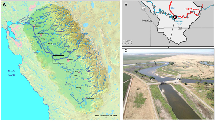
Figure 1. (A) Map of the California Central Valley showing the San Joaquin River as a thick blue line. The area of the SAR demonstration site is depicted by the black rectangle. (B) Zoom-in of the region (rectangle in A) showing the San Joaquin River, the levees and the Chowchilla Canal Bypass (CB). (C) Photograph of the confluence of the Chowchilla Bypass and the San Joaquin River with adjacent farmland (Source: SJR FCPA).

FIGURE 2

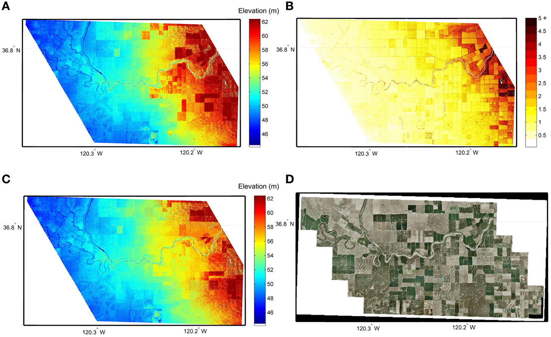
Figure 2. (A) InSAR DEM, linearly calibrated (3 × 3 m). (B) InSAR height precision map in meters (3 × 3 m). (C) InSAR DEM, vegetation corrected (3 × 3 m). (D) Aerial photography of the same area.

This site was identified opportunistically for analysis, as it was collected and processed as part of instrument development. To date, targeted science missions have primarily been over cryospheric targets. However, we believe that this site is a good candidate for rigorously assessing the performance and quality of the InSAR-derived DEM given the high degree of alterations made to the natural floodplain (fields, levees and other numerous man-made structures) to turn the landscape into a prime area for high-end irrigation agriculture. The resulting complexity in terrain features (see Figure 2C) makes it a challenging test case. Further, the availability of a high-resolution LIDAR DEM enables a meaningful comparison against the leading benchmark technology.

2.4. Characterizing Floodplain and River Hydrodynamics

A high-accuracy floodplain DEM is essential for adequate flow modeling and consequently flood risk estimation (Bates, 2004). Substantial errors in the vertical can lead to considerable over- or under-estimation of flood hazard which can have many adverse consequences. Any flood model requires data on river gradients, bank and floodplain heights, and for 1-D in-channel flood models such as HEC-RAS and also for 1-D/2-D coupled flood models this river information is provided as river section data. For this purpose, we assess heights along the stream centerline of the San Joaquin river in flow direction and impose a linear fit to estimate the thalweg gradient and first order hydraulics (i.e., kinematic waveform). To assess the quality of the floodplain topography we run a simple flood-fill algorithm over parts of the 1:100 year floodplain as defined by FEMA. Both analyses are performed on the LiDAR and SAR DEMs, using the former as a reference.

Flood-fill modeling was based on calculating a floodplain elevation profile from the DEM data, which describes floodplain water depth as a function of flooded area (Yamazaki et al., 2011). For simplification depth is given as an increasing function of flooded area so that no local depression is assumed in the floodplain elevation profile. This simplification was based on the assumption that inundation always occurs from lower to higher places within a unit catchment. Prior to this the natural floodplain was delineated using correlation between local valley slope and the topographic wetness index (Beven and Kirkby, 1979), TWI = ln(a∕tan(b)), where high values typically denote converging, almost flat terrain at locations where large upslope areas are drained, a, and where the local gravitational gradient, b, is low.

3. Results

This section reports on the accuracy and overall quality of the GLISTIN-A InSAR DEM and its applicability to flood mapping and modeling. We wish to note that here we present and discuss first findings and, although we believe that the DEM accuracy stated and its suitability to floodplain mapping is transferable to other locations, we suggest more studies of this type to confirm our findings.

3.1. Accuracy Assessment

As outlined in Section 2.1, for swath calibration we used LiDAR data approximately 13 km across-track and we chose an area of no or very low vegetation in both data sets so that we could assume the scene was consistent between collections. Then we filtered the classified vegetation as correcting the height simplistically as described in Section 2.2 and then aggregated the DEM to 30 × 30 m pixels to substantially reduce the noise level. We only aggregated pixels within a 15 m radius that exhibited reasonable height variance (i.e., outliers due to low correlation—water for example—were excluded). This spatial resolution seems more than adequate for floodplain mapping. For instance, meaningful information on inundation maps obtained from a remotely sensed image should preferably have a spatial resolution within a range of 10 m to 1 km depending on the type of application and user needs (Schumann et al., 2012), which is now easily achievable.

Figure 2 displays the slope-corrected InSAR DEM as well as the resulting DEM after vegetation removal, both at a spatial resolution of 3 × 3 m. It should be noted that in some areas (for instance in the upper left corner of Figure 2C) vegetation was not removed because in those areas our crude classifier did not identify these as vegetation. They are likely a different type of vegetation, or the scattering properties differ at the far incidence angles. However, with a more sophisticated automated algorithm this could be improved but it is outside the scope of this paper. Note that, as evidenced in the latter results, the impact of these vegetated regions remaining, remote from the river is insignificant. The final 30 × 30 m InSAR DEM is shown in Figure 3 where height contours are overlain and compared to the LiDAR reference DEM aggregated to the same resolution for a fair assessment. As can be seen in that figure, the InSAR topographic contours are very similar to those derived from the LiDAR, which indicates very similar terrain topology in both datasets.

FIGURE 3

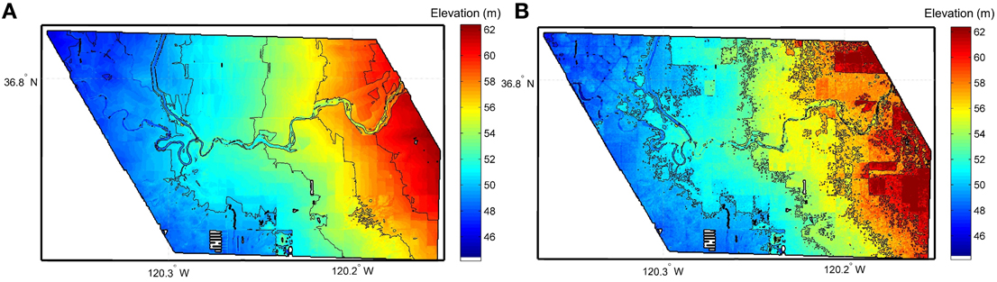
Figure 3. (A) 30 × 30 m aggregated LiDAR bare ground DEM with height contours overlain. (B) The same height interval contours are overlain on the InSAR DEM aggregated to 30 × 30 m after vegetation correction.

For a more quantitative assessment, we also calculated both the bias (systematic error) and the root mean square error (RMSE) between the LiDAR and InSAR floodplain heights. Note that since the LiDAR DEM is a bare ground terrain model, we only selected regions in the InSAR DEM that exhibit little InSAR height precision error and of no or very low vegetation (depicted by red boxes in Figure 4A). The histogram plot in Figure 4B shows the height error with normal distribution around a mean of as low as 5.6 cm with a standard deviation of ±30 cm. When comparing the InSAR DEM to the LIDAR bare ground terrain, the RMSE, which is a standard accuracy metric for DEMs, is 29.7 cm and is given by the following equation:

$\begin{array}{cc}RMSE=\sqrt{\frac{{\displaystyle {\sum }_{n=1}^n{(z_S-z_L)}^2}}{n}},& \left(2\right)\end{array}$

where n is the total number of pixels to be compared and z represents the height in meters of a given pixel with subscripts S and L denoting SAR and LiDAR, respectively.

FIGURE 4

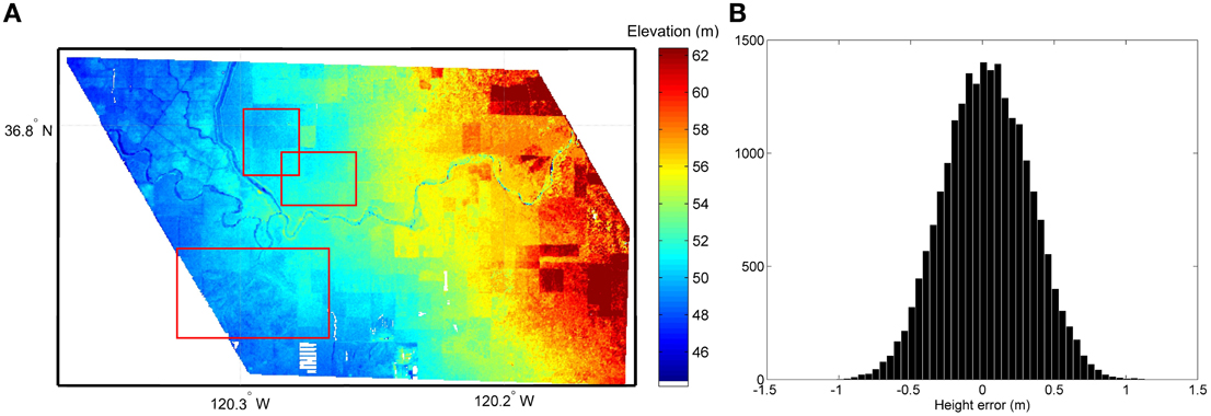
Figure 4. (A) 30 × 30 m InSAR DEM showing subregions used for accuracy assessment (red rectangles). (B) Histogram of relative height error between the final InSAR DEM and the LiDAR bare ground DEM.

3.2. Suitability to Map Floodplain and River Hydrodynamics

We also assessed the suitability of the InSAR DEM for characterizing basic river hydrodynamics and mapping floodplain inundation, as outlined in Section 2.4. It is well known and widely accepted that LiDAR data have been transformative in floodplain mapping and modeling, and raised the expectation that models built using them can predict inundation extent accurately (Bates, 2012).

First order channel hydraulics are typically represented by the kinematic wave form which can be expressed in simple terms as the gradient of the stream centerline. We approximated this gradient using a linear fit to the centerline heights extracted every 30 m along the river thalweg. Unsurprisingly, the LiDAR exhibits the smallest spread along a linear fit (Figure 5) and indicates a downward slope of 28.4 cm per km (typical for a river this size) with an upstream elevation intercept at 54.2 m. The InSAR DEM gives very similar results (slope: 28.9 cm per km; intercept: 54.6 m) while the SRTM DEM, as expected, has a much larger spread of residuals along the gradient line and gives a slope of 23.1 cm per km with an intercept at 56.4 m. Although this can be considered acceptable for the SRTM DEM, errors are typically too large to allow accurate in-channel hydrodynamic modeling.

FIGURE 5

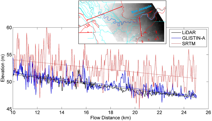
Figure 5. Plot showing the heights along the river centerline in flow direction for the LiDAR, InSAR, and SRTM DEMs. The linear slope is also shown. The inset shows the boundaries of the FEMA 1:100 year flood extent in red and the main river in blue.

In order to demonstrate the suitability to map flooded area on the basis of floodplain height profiling (Yamazaki et al., 2011), we plotted and compared the cumulative distribution function (CDF) of the elevation within the study region of the LiDAR DEM and the InSAR DEM. As shown in Figure 6, there are only marginal differences in the elevation profiles from LiDAR and InSAR. In fact, a two-sample Kolmogorov-Smirnov (KS) test indicates that, at a 5% α level, there are no significant differences between the two floodplain height distributions. The marginal differences become somewhat more important when translating these heights to floodplain inundation as illustrated by the small panels inserted in Figure 6. This is primarily due to the remaining noise in the InSAR DEM rather than actual terrain height discrepancies between the two datasets.

FIGURE 6

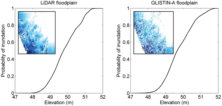
Figure 6. Plot showing the cumulative distribution function of floodplain height profile for both the LiDAR and InSAR DEMs. The small insets show the area inundated to a specific floodplain height for the region inside the lower left rectangle in Figure 4A.

4. Discussion and Preliminary Conclusions

In this paper we assessed and reported the quality and accuracies of a Ka-band single-pass interferometer-derived digital elevation model over a floodplain in the California Central Valley. The NASA airborne mission instrument GLISTIN-A has been designed for ice elevations but here we demonstrated its capability to acquire land elevations at large swath widths with an accuracy comparable to that of state-of-the-art LiDAR. With a RMSE of just under 30 cm compared to LiDAR, we believe these InSAR height data to have much greater vertical accuracies than prior InSAR airborne DEMs, with vertical errors typically about 1 m or larger and rarely smaller than 0.5 m. We also assessed the suitability of the InSAR Ka-band DEM for floodplain inundation mapping and characterizing first order hydrodynamics.

LiDAR is widely considered the best available technology for producing land elevation data. Here, we do not wish to counter-argue this. Instead, we would like to propose an alternative technology of similar accuracy, being able to operate from much higher altitudes, over much wider swaths and during cloudy conditions thereby making it more cost-effective than LiDAR and more suited to acquiring data over large floodplains and coastal regions, and in areas often deprived of LiDAR data.

Despite the several advantages over LiDAR data and its comparable accuracy, we wish to note the following points with regard to the Ka-band InSAR that warrant attention or further analysis:

• InSAR data calibration: If no LiDAR data are available, GPS tie points or satellite altimetry data can be used to calibrate the InSAR data following the method described in Section 2.1.

• Vegetation correction: Note that our method used to remove vegetation, albeit automated and based only on InSAR auxiliary data, is fairly basic and should be improved. Baugh et al. (2013) propose an interesting approach that employs hydrodynamic modeling to guide vegetation height removal on the SRTM DEM. Variants thereof could potentially lead to more sophisticated vegetation correction algorithms for InSAR data. Also, the use of ancillary datasets should be considered.

• Spatial aggregation: SAR data have the inherent property to reduce in noise level when aggregated to lower spatial resolution. Here, we suggested 30 × 30 m from 3 × 3 m pixels but we did not conduct a sensitivity analysis and so the 30 m spatial resolution should only be taken as a guideline. Also, the aggregation method we used is based on variance (Section 3.1) and needs further augmentation. In fact, we suggest developing “intelligent” spatial aggregation/classification methods that conserve micro-topographic features while reducing the noise level for preserving maximum information content.

• Suitability for 2-D flood hazard/risk modeling: Here, we only tested for basic characterization of in-channel hydrodynamics and floodplain inundation mapping and therefore recommend more complete investigations of the suitability of the InSAR data for flood modeling and mapping. In fact what is needed is a proper hydrodynamic modeling benchmark study, preferably using a floodplain and a flood event for which LiDAR data have been used.

• Ongoing technological advances: The GLISTIN-A system represents the first of its kind and was developed for cryospheric mapping. Tailoring a system design to the needs of floodplain mapping, and incorporating relevant recent technology advances will enable superior performance for this application.

Even though there are a number of points that still need improving, most notably in classification and subsequent vegetation removal, based on our findings so far we conclude that the single-pass Ka-band InSAR provides competitive technology to acquire floodplain elevation data with accuracies required for better environmental modeling and risk mapping, especially in developing nations that have very limited or no access to high-quality DEMs.

In order to more fully assess the suitability of the Ka-band InSAR instrument to acquire high-accuracy land elevation data, we suggest to repeat this type of analysis over a more natural floodplain and a larger river, and for an area more prone to regular flooding.

Author Contributions

All authors are in agreement of all aspects of the work published and confirm equal contribution. All authors have contributed equally to the conception and design of the work and drafting of the paper. DM identified the InSAR data, guided the technical analysis and revised the technical parts of the drafting. FM performed the InSAR data calibration and classification. GS did the DEM comparison work and completed the river and floodplain hydrodynamics analysis.

Conflict of Interest Statement

The authors declare that the research was conducted in the absence of any commercial or financial relationships that could be construed as a potential conflict of interest.

Acknowledgments

We would like to acknowledge funding support from the National Aeronautics and Space Administration (NASA, grant number NNX13AD99G) as well as Google Inc. through an Earth Engine Research Award. We would also like to thank the California Department of Water Resources (CA DWR) for providing the LiDAR data and aerial imagery used in this study. At the NASA Jet Propulsion Laboratory we would like to acknowledge Drs. Scott Hensley and Xiaoqing Wu, and the GLISTIN-A and UAVSAR teams.

References

Bates, P. D. (2004). Invited commentary: remote sensing and flood inundation modelling. Hydrol. Process. 18, 2593–2597. doi: 10.1002/hyp.5649

CrossRef Full Text | Google Scholar

Bates, P. D. (2012). Invited Commentary: integrating remote sensing data with flood inundation models: how far have we got? Hydrol. Process. 26, 2515–2521. doi: 10.1002/hyp.9374

CrossRef Full Text | Google Scholar

Baugh, C. A., Bates, P. D., Schumann, G., and Trigg, M. A. (2013). Srtm vegetation removal and hydrodynamic modeling accuracy. Water Resour. Res. 49, 5276–5289. doi: 10.1002/wrcr.20412

CrossRef Full Text | Google Scholar

Beven, K. J., and Kirkby, M. J. (1979). A physically based, variable contributing area model of basin hydrology. Hydrol. Sci. Bull. 24, 43–69. doi: 10.1080/02626667909491834

CrossRef Full Text | Google Scholar

Cobby, D. M., Mason, D. C., and Davenport, I. J. (2001). Image processing of airborne scanning laser altimetry data for improved river flood modelling. ISPRS J. Photogramm. Remote Sens. 56, 121–138. doi: 10.1016/S0924-2716(01)00039-9

CrossRef Full Text | Google Scholar

Cobby, D. M., Mason, D. C., Horritt, M. S., and Bates, P. D. (2003). Two-dimensional hydraulic flood modelling using a finite-element mesh decomposed according to vegetation and topographic features derived from airborne scanning laser altimetry. Hydrol. Process. 17, 1979–2000. doi: 10.1002/hyp.1201

CrossRef Full Text | Google Scholar

Friant Water Users Authority (2002). San Joaquin River Restoration Study: Background Report. Final Report, Friant Water Users Authority, Natural Resources Defense Council.

Hallegatte, S., Green, C., Nicholls, R. J., and Corfee-Morlot, J. (2013). Future flood losses in major coastal cities. Nat. Clim. Change 3, 802–806. doi: 10.1038/nclimate1979

CrossRef Full Text | Google Scholar

Moller, D., Hensley, S., Sadowy, G. A., Fisher, C. D., Michel, T., Zawadzki, M., et al. (2011). The glacier and land ice surface topography interferometer: an airborne proof-of-concept demonstration of high-precision ka-band single-pass elevation mapping. IEEE Trans. Geosci. Remote Sens. 49, 827–842. doi: 10.1109/TGRS.2010.2057254

CrossRef Full Text | Google Scholar

Neal, J. C., Schumann, G., and Bates, P. D. (2012). A subgrid channel model for simulating river hydraulics and floodplain inundation over large and data sparse areas. Water Resour. Res. 48:W11506. doi: 10.1029/2012WR012514

CrossRef Full Text | Google Scholar

NIH (2010). Human Genome Project. Fact Sheet, National Institutes of Health. Available online at: http://report.nih.gov/NIHfactsheets/Pdfs/HumanGenomeProject

Rodriguez, E., and Martin, J. M. (1992). Theory and design of interferometric synthetic-aperture radars. Proc. IEEE 139, 147–159. doi: 10.1049/ip-f-2.1992.0018

CrossRef Full Text | Google Scholar

Rosen, P. A., Hensley, S., Joughin, I. R., Li, F. K., Madsen, S. N., Rodriquez, E., et al. (2000). Synthetic aperture radar interferometry. Proc. IEEE 88, 333–382. doi: 10.1109/5.838084

CrossRef Full Text | Google Scholar

Sanders, B. F. (2007). Evaluation of on-line DEMs for flood inundation modeling. Adv. Water Resour. 30, 1831–1843. doi: 10.1016/j.advwatres.2007.02.005

CrossRef Full Text | Google Scholar

Schumann, G. J.-P., Bates, P. D., Baldassarre, G. D., and Mason, D. C. (2012). “The use of radar imagery in riverine flood inundation studies,” in Fluvial Remote Sensing for Science and Msnagement, eds P. E. Carbonneau and H. Piégay (Chichester, UK: Wiley-Blackwell). 115–140.

Schumann, G. J.-P., Bates, P. D., Neal, J. C., and Andreadis, K. M. (2014). Fight floods on a global scale. Nature 507, 169. doi: 10.1038/507169e

PubMed Abstract | CrossRef Full Text | Google Scholar

Schumann, G. J.-P., Neal, J. C., Voisin, N., Andreadis, K. M., Pappenberger, F., Phanthuwongpakdee, N., et al. (2013). A first large scale flood inundation forecasting model. Water Resour. Res. 49, 6248–6257. doi: 10.1002/wrcr.20521

CrossRef Full Text | Google Scholar

Yamazaki, D., Kanae, S., Kim, H., and Oki, T. (2011). A physically based description of floodplain inundation dynamics in a global river routing model. Water Resour. Res. 47:W04501. doi: 10.1029/2010WR009726

CrossRef Full Text | Google Scholar