Spatial Patterns of Sea Surface Temperature Influences on East African Precipitation as Revealed by Empirical Orthogonal Teleconnections
 Tim Appelhans
 Thomas Nauss
- Environmental Informatics, Department of Geography, Philipp University of Marburg, Marburg, Germany
East Africa is characterized by a rather dry annual precipitation climatology with two distinct rainy seasons. In order to investigate sea surface temperature driven precipitation anomalies for the region we use the algorithm of empirical orthogonal teleconnection analysis as a data mining tool. We investigate the entire East African domain as well as 5 smaller sub-regions mainly located in areas of mountainous terrain. In searching for influential sea surface temperature patterns we do not focus any particular season or oceanic region. Furthermore, we investigate different time lags from 0 to 12 months. The strongest influence is identified for the immediate (i.e., non-lagged) influences of the Indian Ocean in close vicinity to the East African coast. None of the most important modes are located in the tropical Pacific Ocean, though the region is sometimes coupled with the Indian Ocean basin. Furthermore, we identify a region in the southern Indian Ocean around the Kerguelen Plateau which has not yet been reported in the literature with regard to precipitation modulation in East Africa. Finally, it is observed that not all regions in East Africa are equally influenced by the identified patterns.
1. Introduction
In contrast to other tropical areas, East Africa is characterized by a rather dry annual precipitation climatology. Rainfall exhibits a strong seasonal signal with two distinct rainy seasons throughout the year (Yang et al., 2014). The major rainy season, the so-called “long rains” is from March until May (MAM), while the second rainy season from October to December (OND), the “short rains” is more variable but usually centered around November. The modulation of these rainy seasons by regional to global sea surface temperature (SST) anomalies has been the focus of numerous studies in the past (e.g., Rocha and Simmonds, 1997; Mutai et al., 1998; Latif et al., 1999; Plisnier et al., 2000; Behera et al., 2005; Black, 2005; Marchant et al., 2007; Ummenhofer et al., 2009; Manatsa et al., 2012, 2014; Manatsa and Behera, 2013; Bahaga et al., 2015; Tierney et al., 2015). From these studies it becomes evident that, at least for the “short rains,” the Indian Ocean Dipole (IOD) plays a much bigger role than the El Nino Southern Oscillation (ENSO) in East Africa. There is, however, a clear tendency of most of these studies to (i) focus on particular seasons and/or (ii) focus on the influences of one or two predefined (coupled) ocean (-atmosphere) indeces such as IOD or ENSO to name the two most widely investigated for this area. There are, to the best of our knowledge, no climatological studies that have approached SST induced precipitation influences over East Africa in a holistic, data driven manner up to now. Furthermore, most studies investigate SST-precipitation linkages for a rather broad regional area lacking conclusions on local scales. We intend to fill these gaps by investigating potential SST driven precipitation anomalies for (i) the complete time interval between 1982 and 2010 and (ii) for several sub-regions of about 100 × 100 km in addition to the entire East African domain. So far, few studies exist that link SST influences and eco-climatological anomalies for selected local regions in East Africa such as Chan et al. (2008); Otte et al. (personal communication) for Mt. Kilimanjaro, but these are often based on in situ rain gauge observations which limit their area-wide significance, even for the rather small local domain. In this study, we approach the SST driven precipitation anomalies at Mt. Kilimanjaro in a spatially and temporally holistic manner. Area-wide high-resolution precipitation grids (see next section for details) are being used over the complete period between 1982 and 2010, not limiting the investigation to any seasonal period.
2. Materials and Methods
2.1. Data
Monthly SSTs between 60°N and 60°S for the entire globe are obtained from the NOAA SST product (NOAA OI SST V2, Reynolds et al., 2007). For precipitation information we use monthly Climate Hazards Group Infra Red Precipitation with Station data (CHIRPS) version 2.0 (Funk et al., 2014). CHIRPS is a 30+ year quasi global rainfall data set, which is available from 1981 until the recent present and has a resolution of 0.05° × 0.05° (longitude × latitude). It incorporates a number of satellite precipitation products including Tropical Rainfall Measuring Mission (TRMM), rainfall fields from NOAA's Climate Forecast System version 2 (CFSv2) as well as in situ precipitation observations. For a detailed description of the incorporated data and the applied methodology for the creation of CHIRPS, the reader is referred to Funk et al. (2014). Figure 1 gives an overview of the precipitation domains used in this study. In addition to the entire East African region we also investigate SST driven precipitation anomalies for five small mountainous sub-regions, namely Lake Tana, Bale Mountains, Mt. Kenya, Mt. Kilimanjaro and Mt. Loleza (from North to south) to investigate whether local differences in identified patterns can be observed. Note that for the entire East African domain CHIRPS data was re-sampled to 0.25° × 0.25° (longitude × latitude) to ensure acceptable computation times. Prior to the analysis, both data sets were tested for potential break points potentially stemming from changing observational input data over time. No such breakpoints were found in either data set.
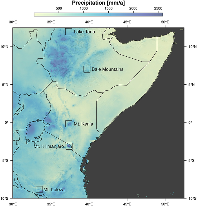
Figure 1. Mean annual precipitation between 1982 and 2010 in the response domains. Black squares show the locations of the small response domains.
2.2. Methods
In order to identify the influence of SST anomalies on East African rainfall we use Empirical Orthogonal Teleconnection (EOT) analysis as described in Appelhans et al. (2015). EOTs have first been introduced to the international literature as an alternative to the classical approach of Empirical Orthogonal Functions (EOF) by van den Dool et al. (2000) who outlines that both EOT and EOF are indeed very similar techniques with the former producing less abstract results. EOTs carry a quantitative meaning in the form of explained variance, thus enabling intuitive interpretation of the results. In brief, the algorithm works as follows:
1. Each pixel of the predictor domain time series is regressed against all pixels of the response domain time series.
2. The predictor pixel with the highest sum in the coefficients of determination is identified as the base point of the first mode.
3. All pixels of the predictor and response domains are then again regressed against this base point to quantify the relationships between this point and the rest of the domains.
4. To identify further modes, steps 1–3 are repeated on the residuals of the preceding mode, thus ensuring orthogonality.
These steps can be repeated until a desired number of modes is identified. Apart from similarity in the temporal dimension (i.e., identical amount of data points over time), the algorithm can be applied to any two data series without any requirements such as identical spatial resolution or physical units of the data. For detailed descriptions of the mathematics behind EOT analysis the reader is referred to van den Dool et al. (2000) and van den Dool (2007). Here, we use SSTs as the predictor series and precipitation as the response series and limit our investigation to the first two modes. Both data sets were pre-processed to extract climatic signals inherent in the time series. Seasonality was removed by subtracting the long term monthly mean. Background noise within the series was removed by principal component analysis (PCA), keeping those components that describe just above 80% of the time series inherent variance. Potential linear trends in the data sets were not removed as we explicitly want to capture possible changes in the relationships between the two data sets over time. In total we analyze 29 years of monthly SST and precipitation anomalies for the time period 1982–2010. We apply the EOT approach to moving chunks of 5 years of monthly observations. This is first carried out for the 60 time slices between 1982 and 1986. Then the application window is moved forward by 1 year so that the analysis is repeated with the next set of observations ranging from 1983 to 1987. This procedure is repeated until the last available 5 year chunk between 2006 and 2010 is analyzed producing 24 sets of modes between 1982 and 2010 in total. For each of these chunks we analyze temporal lags between SSTs and precipitation from 0 to 12 months.
3. Results
In this section we focus on the description of the results found for the entire East African domain and provide references to the corresponding findings within the sub-domains (see Supplementary Materials) where approproate. For each domain we identify a total of 624 base points (24 chunks * 13 lags * 2 modes) and associated SST regions, represented by the coefficients of determination between the base points and each pixel in the SST domain. In order to understand the temporal dynamics of these patterns, Figure 2 provides an overview over the combined explanatory power of modes 1 + 2 over all 312 chunk/lag combinations analyzed for the East African domain (left panel) and the corresponding correlation coefficients for mode 1 (center panel) and mode 2 (right panel) individually. The solid white squares highlight the 16 modes with highest explanatory power (the upper 0.95 quantile of explained variance in the left panel). In general, and irrespective of lag times, the 1980s, early 1990s and early 2000s reveal reduced influence, while the mid to late 1990s and mid to late 2000s show enhanced explanatory power. All of the 16 most important chunk/lag combinations occur during these periods. A detailed overview of the identified patterns for the 16 most dominant base points is given in Figures 4, 5 for the leading modes and their respective secondary modes. It becomes evident that some of these patterns are rather solitary occurrences, e.g., “1995–1999 lag12,” “2001–2005 lag12,” and “2003–2007 lag00.” The latter clearly shows the influence of a positive IOD event in mode 1, which is also the mode that provides the vast majority of the explanatory power as can be seen in Figure 2. In line with previous studies, this positive IOD phase related mode exhibits the strongest absolute influence in our analysis. Given the close vicinity of the SST pattern to the response domain this is hardly surprising. In addition to these solitary patterns, we see a few patterns evolving that occur at least twice (indicated by the small letters in Figure 2). This is, however, only true for the leading modes in Figure 4. The second modes shown in Figure 5 do not show any pattern consistency neither related to the leading modes, nor overall. This is true for all domains as can be seen in the respective figures in the Supplementary Materials. Figure 3 provides an overview of these labeled patterns averaged over all mode 1 occurrences together with the respective averaged correlation coefficients in the response domain. We see that the shortest lag time is found in the Indian Ocean (Figure 3a). This pattern is related to the negative phase of the IOD exhibiting negative correlation to East African rainfall. This pattern is also found for the smaller domains that are located near or south of the equator, namely Mt. Kenya, Mt. Kilimanjaro and Mt. Loleza even though the lag times differ slightly (see Figures S10a, S14a, and S18a in Supplementary Materials). Pattern 3b with a lag of 8 to 9 months is located in the extra-tropical Indian Ocean and is positively correlated with East African precipitation. The location just north of the Kerguelen Islands indicates that the Antarctic Polar Front plays a role here. Moore et al. (1999) report consistent modulation of SSTs around the Kerguelen Plateau, a large sub-marine topographical feature that poses a natural obstacle for the Antarctic Circumpolar Current (ACC). To the best of our knowledge, there are no previous studies linking this oceanic region to East African climate. Yet, this is the only pattern we see in the large East African domain as well as in all small sub-domains, which highlights its importance for the region. Pattern 3c is located in the equatorial Atlantic and has a lag of 5–6 months. It is negatively correlated with East African precipitation and the only sub-domain to also reveal this pattern is the one surrounding Mt. Kenya. Pattern 3d with 9–10 months lag is located in the southern subtropical Atlantic Ocean and shows negative correlation coefficients with the response domain. In comparison to the other negatively correlated patterns, this exhibits the strongest signal, especially in the East African lowlands. This pattern as such is not found in any of the sub-domains, yet Lake Tana and Bale Mountains exhibit a similar pattern both in terms of location and lag times indicating that this pattern mainly influences the northern parts of the East African region. Pattern 3e is located in the south-eastern subtropical Pacific and is lagged by 10 months. Given that no sub-domain exhibits any patterns similar to this positively correlated influence on East Africa, it may be that this pattern is especially important for the lower elevated regions throughout the domain, as all our sub-domains are domains of complex terrain.
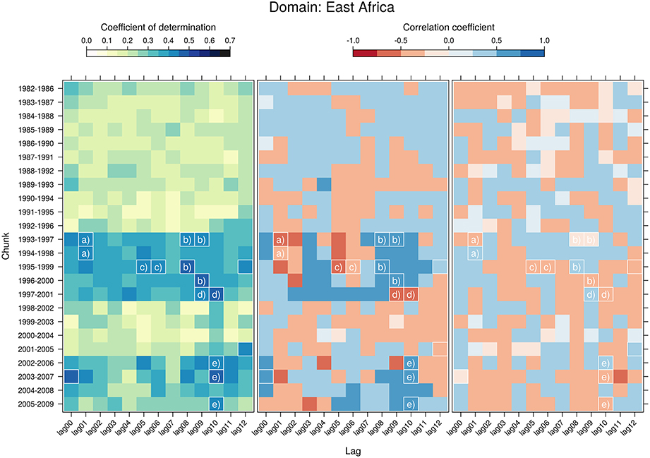
Figure 2. Left: Explained space-time variance of the East African response domain for modes 1 and 2 by chunk and lag. Center: Mean correlation coefficient between the identified base point and all pixels in the response domain by chunk and lag for mode 1. Right: Mean correlation coefficient between the identified base point and all pixels in the response domain by chunk and lag for mode 2. Labels a–e show the chunk/lag combinations that are used in Figure 3. Solid white squares denote upper 0.95 quantile in explained variance.
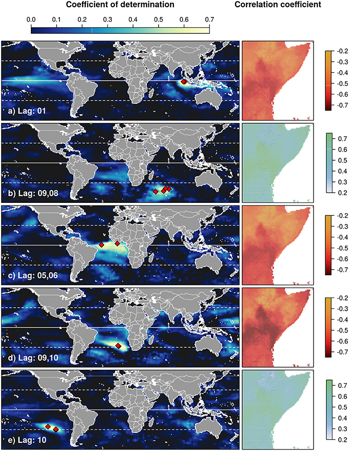
Figure 3. The five most important SST regions for the East African domain as indicated by the small letters in Figure 2. Left panels show mean coefficient of determination between each pixel of the predictor domain and the respective base points (red diamonds). Right panels show average correlation coefficient between each pixel in the response domain and the respective base points. Lag times are provided in the lower left corner of the left panels.
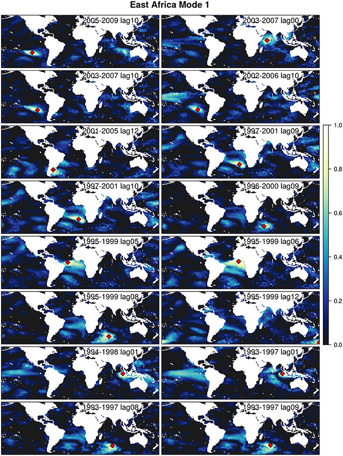
Figure 4. The 16 most important patterns in mode 1 (upper 0.95 quantile in explained variance) as identified by the white squares in Figure 2.
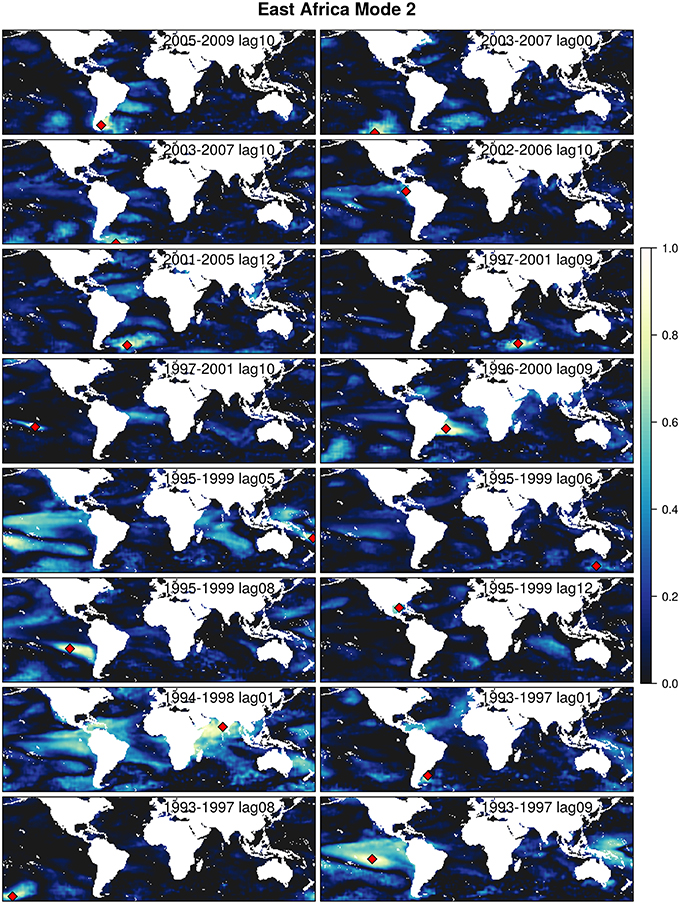
Figure 5. The 16 most important patterns in mode 2 (upper 0.95 quantile in explained variance) as identified by the white squares in Figure 2.
Regarding the East African lowland regions, it is generally observed that the correlations are higher for these areas than for the areas of complex terrain, regardless of domain size, pattern location or lag times. One potential reason for this could be found in the nature of the data, with gridded data being generally less accurate over areas of more heterogeneous topography. A further general observation is that the two oceanic basins surrounding the African continent seem to play a bigger role than the tropical Pacific Ocean, though isolated patterns do exist and it is sometimes coupled which point to influences from this basin. Regarding the consistency between first and second modes, which, if found, would indicate teleconnectivity, we do not find any patterns that re-occur within the second mode as they do in the first in any of the domains. This indicates that, should such precipitation modulating teleconnections between oceanic regions exist, they operate on temporal scales beyond the five year chunks that we have investigated here.
4. Discussion
In this study we have used empirical orthogonal teleconnection analysis to identify global sea surface temperature regions that influence precipitation in East Africa and selected montane sub-regions within the region. We did not limit our analysis to any season or any region, rather we investigated SST influences in 5 year chunks for the entire period between 1982 and 2010 and lag times between 0 and 12 months. Our approach does not enable any process inference as it is purely statistical. There has been much focus in the international literature on understanding the dynamic links between IOD and ENSO and East African precipitation. Here, we found that the region around the Kerguelen Plateau in the southern Indian Ocean plays a role throughout the entire East African domain, regardless of scale, which has not been reported in the literature before. Furthermore, we found (i) that there are distinct times of enhanced influences, (ii) that the most influential SST regions are located in the Indian and Atlantic Ocean basins, (iii) that the Indian Ocean Dipole exhibits highest explanatory power with regard to precipitation modulation in East Africa, (iv) that not all identified influences are equally important throughout the East African domain and (v) that lowland areas are generally more influenced than mountainous regions. Our findings suggest that any inference of previously reported SST influences on East African precipitation need to be carefully tested when applied to smaller areas within the region as it can not be assumed that these will be of equal importance throughout the entire domain. This is also true for considerations over time. From our analysis it becomes evident that influential SST regions shift depending on the considered time span. Therefore, assumptions about regional SST influences in East Africa should be carefully considered when applied to investigations on local spatial and differing temporal scales. In addition, topography also influences correlations so that this aspect needs to be considered as well. In light of the identified influential region around the Kerguelen Plateau, we suggest that this region be investigated more closely in the future, especially regarding the processes underlying this link to precipitation in the East African region. Our findings suggest that there are other regions that do also play a role in influencing precipitation over the region and it would be desirable to understand the driving processes at a similar level of detail as we already do for IOD and ENSO.
Author Contributions
TA performed all analyses and wrote most of the manuscript. TN significantly contributed to the final submitted manuscript version.
Conflict of Interest Statement
The authors declare that the research was conducted in the absence of any commercial or financial relationships that could be construed as a potential conflict of interest.
Acknowledgments
This work was carried out in the frame work of of the DFG-Research Unit 1246 KiLi - Kilimanjaro ecosystems under global change: Linking biodiversity, biotic interactions and bio-geochemical ecosystem processes. funded by the German Research Foundation (DFG, funding ID Ap 243/1-2, Na 783/5-1, Na 783/5-2). We are grateful for the contructive reviewer feedback which were very helpful and improved the quality of the manuscript significantly.
Supplementary Material
The Supplementary Material for this article can be found online at: https://www.frontiersin.org/article/10.3389/feart.2016.00003
References
Appelhans, T., Detsch, F., and Nauss, T. (2015). remote: Empirical orthogonal teleconnections in r. J. Stat. Softw. 65, 1–19. doi: 10.18637/jss.v065.i10
Bahaga, T. K., Mengistu Tsidu, G., Kucharski, F., and Diro, G. T. (2015). Potential predictability of the sea-surface temperature forced equatorial east african short rains interannual variability in the 20th century. Q. J. R. Meteorol. Soc. 141, 16–26. doi: 10.1002/qj.2338
Behera, S. K., Luo, J.-J., Masson, S., Delecluse, P., Gualdi, S., Navarra, A., et al. (2005). Paramount impact of the indian ocean dipole on the east african short rains: a cgcm study. J. Clim. 18, 4514–4530. doi: 10.1175/JCLI3541.1
Black, E. (2005). The relationship between Indian Ocean sea-surface temperature and East African rainfall. Philos. Trans. A Math. Phys. Eng. Sci. 363, 43–47. doi: 10.1098/rsta.2004.1474
Chan, R. Y., Vuille, M., Hardy, D. R., and Bradley, R. S. (2008). Intraseasonal precipitation variability on Kilimanjaro and the East African region and its relationship to the large-scale circulation. Theor. Appl. Climatol. 93, 149–165. doi: 10.1007/s00704-007-0338-9
Funk, C., Peterson, P., Landsfeld, M., Pedreros, D., Verdin, J., Rowland, J., et al. (2014). A Quasi-Global Precipitation Time Series for Drought Monitoring. Technical Report 4, U.S. Geological Survey Data Series.
Latif, M., Dommenget, D., Dima, M., and Grötzner, A. (1999). The role of indian ocean sea surface temperature in forcing east african rainfall anomalies during decemberjanuary 1997/98. J. Clim. 12, 3497–3504.
Manatsa, D., and Behera, S. K. (2013). On the epochal strengthening in the relationship between rainfall of east africa and iod. J. Clim. 26, 5655–5673. doi: 10.1175/JCLI-D-12-00568.1
Manatsa, D., Chipindu, B., and Behera, S. (2012). Shifts in iod and their impacts on association with east africa rainfall. Theor. Appl. Climatol. 110, 115–128. doi: 10.1007/s00704-012-0610-5
Manatsa, D., Morioka, Y., Behera, S., Matarira, C., and Yamagata, T. (2014). Impact of mascarene high variability on the east african short rains. Clim. Dyn. 42, 1259–1274. doi: 10.1007/s00382-013-1848-z
Marchant, R., Mumbi, C., Behera, S., and Yamagata, T. (2007). The indian ocean dipole the unsung driver of climatic variability in east africa. Afr. J. Ecol. 45, 4–16. doi: 10.1111/j.1365-2028.2006.00707.x
Moore, J. K., Abbott, M. R., and Richman, J. G. (1999). Location and dynamics of the antarctic polar front from satellite sea surface temperature data. J. Geophys. Res. Oceans 104, 3059–3073. doi: 10.1029/1998JC900032
Mutai, C., Ward, M., and Colman, W. (1998). Towards the prediction of the East Africa short rains based on sea surface temperature atmosphere coupling. Int. J. Climatol. 18, 975–997.
Plisnier, P., Serneels, S., and Lambin, E. (2000). Impact of enso on east african ecosystems: a multivariate analysis based on climate and remote sensing data. Glob. Ecol. Biogeogr. 9, 481–497. doi: 10.1046/j.1365-2699.2000.00208.x
Reynolds, R. W., Smith, T. M., Liu, C., Chelton, D. B., Casey, K. S., and Schlax, M. G. (2007). Daily high-resolution-blended analyses for sea surface temperature. J. Clim. 20, 5473–5496. doi: 10.1175/2007JCLI1824.1
Rocha, A., and Simmonds, I. (1997). Interannual Variability of South-Eastern African Summer Rainfall. Part 1: Relationships With AirSea Interaction Processes. Int. J. Climatol. 17, 235–265.
Tierney, J. E., Ummenhofer, C. C., and deMenocal, P. B. (2015). Past and future rainfall in the horn of africa. Sci. Adv. 1:e1500682. doi: 10.1126/sciadv.1500682
Ummenhofer, C. C., Gupta, A. S., and England, M. H. (2009). Contributions of Indian Ocean Sea surface temperatures to enhanced East African rainfall. J. Clim. 22, 993–1013. doi: 10.1175/2008JCLI2493.1
van den Dool, H., Saha, S., and Johansson, R. (2000). Empirical orthogonal teleconnections. J. Clim. 13, 1421–1435. doi: 10.1175/1520-0442(2000)013<1421:EOT>2.0.CO;2
van den Dool, H. M. (2007). Empirical Methods in Short-Term Climate Prediction. Oxford; New York: Oxford University Press.
Keywords: climatology, sea surface temperatures, precipitation, Kilimanjaro, empirical orthogonal teleconnection
Citation: Appelhans T and Nauss T (2016) Spatial Patterns of Sea Surface Temperature Influences on East African Precipitation as Revealed by Empirical Orthogonal Teleconnections. Front. Earth Sci. 4:3. doi: 10.3389/feart.2016.00003
Received: 29 August 2015; Accepted: 11 January 2016;
Published: 09 February 2016.
Edited by:
Jing-Jia Luo, Australian Bureau of Meteorology, AustraliaCopyright © 2016 Appelhans and Nauss. This is an open-access article distributed under the terms of the Creative Commons Attribution License (CC BY). The use, distribution or reproduction in other forums is permitted, provided the original author(s) or licensor are credited and that the original publication in this journal is cited, in accordance with accepted academic practice. No use, distribution or reproduction is permitted which does not comply with these terms.
*Correspondence: Tim Appelhans, tim.appelhans@gmail.com