Estimating Permafrost Distribution in the Maritime Southern Alps, New Zealand, Based on Climatic Conditions at Rock Glacier Sites

Introduction

Alpine permafrost distribution studies have focused predominantly on continental regions, building on pioneering work in the European Alps (e.g., Haeberli, 1975; Barsch, 1978) and the North American Cordilleras (e.g., Wahrhaftig and Cox, 1959; Ives and Fahey, 1971; Harris and Brown, 1978). Consequently, permafrost distribution estimates for maritime climates are underrepresented in the literature. An oceanic control on permafrost distribution limits has been occasionally suggested in the past. Cheng (1983) found altitudinal permafrost limits in Western China were lower in areas of lower continentality due to the effect of cloud cover (more frequent in maritime climates) at latitudes below 40°N. Gorbunov (1978) reported a general trend of lower mountain permafrost limits in littoral regions without elaborating on possible controls. Similarly, Matsuoka (2003) documented lower permafrost limits in Asian high mountain areas of humid continental and pacific climate than in arid continental climates. Conversely, Gruber and Haeberli (2009) suggested an increase in elevation of permafrost limits on gentle slopes toward maritime areas, where thick insulating snowpacks result in warmer temperatures in the underlying substrate. More information on permafrost distribution in maritime settings is needed to further explore the existing, partly contradictory, understanding of permafrost occurrence in maritime areas.

Regional estimates of permafrost distribution are frequently based on rock glaciers, which are the largest and most conspicuous permafrost indicators in alpine environments (e.g., Barsch, 1996; Haeberli et al., 2006). Rock glaciers are slope-scale features that form by the gravity-driven creep of ice-oversaturated talus or till. Their surface commonly exhibits a characteristic ridge-and-furrow topography, created by longitudinal compression and buckle folding due to increased friction toward the margins or at slope changes (e.g., Frehner et al., 2015). Both size and surface morphology make rock glaciers easily identifiable in remotely sensed imagery. Depending on the rock glacier's mobility and permafrost presence, three activity states are distinguished: active (containing ice, moving), inactive (containing ice, not moving), and relict rock glaciers (not containing ice, not moving). The presence of permafrost is strongly dependent on a suitably cold climate (e.g., Haeberli et al., 2010). Consequently, the spatial distribution of active, inactive, and relict rock glaciers has been found to correlate with elevation and aspect (e.g., Brazier et al., 1998; Janke, 2007; Lilleøren and Etzelmüller, 2011), reflecting spatial variations in temperature and insolation.

Research on the geographic extent of permafrost in New Zealand's Southern Alps has been limited (cf. Augustinus, 2002). A first rock glacier inventory aiming at the description of the Southern Alps' permafrost extent was created by Jeanneret (1975), who mapped 27 active rock glaciers in selected areas and found frontal lobe altitudes ranging between 1620 and 2180 m above sea level (asl). Based on a more comprehensive rock glacier inventory for the Ben Ohau Range, Brazier et al. (1998) proposed a lower limit of ~2000 m asl for sporadic permafrost occurrences in the Southern Alps, supporting an earlier estimate by Gorbunov (1978) based on first-order snowline approximations. Allen et al. (2008) adapted Haeberli's (1975) topoclimatic distribution thresholds for steep slopes (>20°) to the climatic conditions in the Mt Cook region, but found that this model underestimated the permafrost extent indicated by rock glaciers in the region. A second model by Allen et al. (2009) focused on estimating permafrost distribution in steep rockwalls by modeling mean annual rock temperatures and suggested that bedrock permafrost may occur in extremely shaded locations as low as ~2000 m asl.

Existing empirical distribution estimates for the Southern Alps provide altitudinal limits derived either from permafrost observations in a single mountain range or from a few selected sites from multiple ranges. A regional-scale permafrost estimate for the Southern Alps, based on a spatially extensive observation inventory, is so far missing. Gruber (2012) recently presented a first-order estimate of the geographic extent of permafrost in New Zealand as part of a global permafrost zonation model based on relationships between permafrost extent and long-term mean annual air temperature (MAAT). This model has yet to be evaluated with local observations.

In this paper, we present an empirical, spatially-distributed permafrost estimate for debris-mantled slopes in the maritime Southern Alps based on a spatially-extensive rock glacier inventory that covers a significant proportion of the mountain chain's high-altitude areas. We compare our predictions to permafrost distributions in more continental regions to evaluate whether a maritime influence on permafrost occurrence in New Zealand is present.

Study Area

The Southern Alps are an elongate southwest-trending mountain chain on the South Island of New Zealand (Figure 1). The mountain belt, created by the oblique collision of the Pacific and Australian plates, is ~800 km long, 60 km wide, and consists of a series of ranges and basins (Barrell et al., 2011). Many mountains along and close to the Southern Alps' drainage divide, referred to as the Main Divide, rise above 2500 m asl, including New Zealand's highest mountain, Aoraki/Mt Cook (3724 m; Sirguey, 2014). The extent of the Southern Alps has not been officially defined. In this paper, we refer to all South Island mountain ranges created by tectonic transpression as the Southern Alps, including the Kaikoura ranges in the north (Figure 1).

FIGURE 1

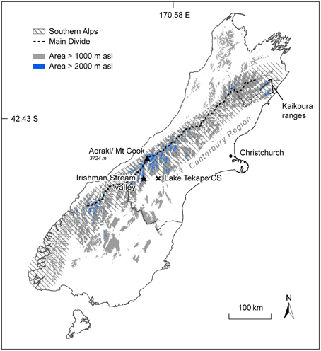
Figure 1. Extent of the Southern Alps on New Zealand's South Island, as defined in this paper, and locations mentioned in the text. Elevation data: 25 m DEM, Barringer et al. (2002), coastline and regional boundaries: Statistics New Zealand (2013).

The climate of the Southern Alps is temperate with a strong maritime influence (cf. Sturman and Wanner, 2001). The Southern Alps' orientation perpendicular to the prevailing moisture-laden westerly winds creates a strong orographic precipitation regime on a regional scale, inducing increasingly “continental” climate toward the east. However, the annual range of mean monthly temperatures at Lake Tekapo, one of the most continental sites in the Southern Alps, is only 13.5°C (1971–2000; NIWA, 2010), a several degrees smaller range than in the central European Alps (Figure 2), demonstrating that the maritime influence in New Zealand is pervasive.

FIGURE 2

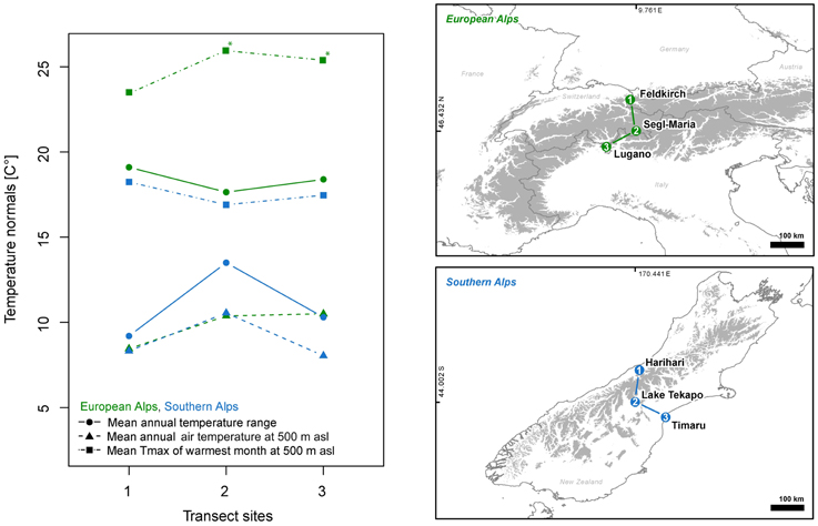
Figure 2. Comparison of mean annual temperature range (i.e, difference between the mean air temperatures of the warmest and coldest month), mean annual air temperature extrapolated to 500 m asl (using the standard environmental lapse rate of 6.5° km⁻¹, Barry, 2008), and mean daily maximum temperature (Tmax) of the warmest month extrapolated to 500 m asl for three climate stations in the New Zealand Southern Alps and three climate stations in the European Alps. New Zealand stations: Harihari, ID 4044, 43.144 S 170.553 E, 45 m asl; Lake Tekapo, ID 4970, 44.002 S 170.441 E, 762 m asl; Timaru, ID 5095, 44.412 S 171.254 N, 17 m asl; NZ data source: NIWA, 2010; European stations: Feldkirch, 47.267 N 9.6 E, 439 m asl, source: ZAMG, 2002; Segl-Maria, ID 24, 46.43 N 9.76 E, 1804 m asl; Lugano, ID 47, 46.00 N 8.96 E, 273 m asl, Swiss data source: MeteoSchweiz, 2014. Temperature normals are derived from homogenized data series for the standard climate period 1971–2000, with the exception of mean maximum temperatures for the Swiss stations Segl-Maria and Lugano (marked with *), which were only available in homogenized form for the climate period 1981–2010. Maps: Elevation data (area > 1000 m asl): WorldClim's elevation dataset (Hijmans et al., 2005), country boundaries: Global Administrative Areas database V2.8 (GADM, 2015).

Annual precipitation is highest on the western flank near the Main Divide (up to 14 m a⁻¹, Henderson and Thompson, 1999) and immediately east of the Main Divide due to spillover (cf. Sinclair et al., 1997). Further eastwards, annual rainfall totals drop to <1000 mm in the inland mountain basins and on the eastern plains (Griffiths and McSaveney, 1983). Modern glacial equilibrium line altitudes in the central Southern Alps rise from 1600 m asl west of the Main Divide to 2000–2200 m asl on eastern glaciers (Lamont et al., 1999), mimicking this precipitation gradient. In the Inland Kaikoura Range, at the northern extreme of the Southern Alps, the present glacial equilibrium line altitude is estimated at 2500 m asl (Chinn, 1995).

Methods

To construct a permafrost estimate for the Southern Alps, we first compiled a rock glacier inventory as an indicator of permafrost presence or absence. We then quantified the relationship between permafrost presence and the topoclimatic controls MAAT and potential incoming solar radiation (hereafter referred to as solar radiation) using logistic regression. From these statistical relationships, we developed a catchment-scale distributed predictive model for debris-mantled slopes. This model calculates the permafrost probability at a given location based on local estimates of MAAT and solar radiation. Last, we evaluated the model output using end-of-winter equilibrium temperature at the snowpack base (i.e., a constant ground surface temperature developing toward the end of winter underneath an insulating snow cover; hereafter referred to as winter equilibrium temperature) as an independent indicator of local permafrost occurrence.

Compilation of a Rock Glacier Inventory

Talus-derived rock glaciers occur in the Southern Alps in high-altitude areas east of the Main Divide, where the climate is cold enough for the preservation of perennially frozen ground but too dry for glaciers to occupy topographically suitable locations (e.g., Humlum, 1998). For rock glacier mapping, we concentrated on the Southern Alps' central ranges between 44.32° S and 42.95° S as well as the Inland Kaikoura Range (42° S). A preliminary survey of satellite imagery showed that almost all of the permafrost creep features in the Southern Alps are located in these regions.

We chose the rock glacier initiation line [Humlum, 1998; corresponding to Barsch's, 1996 “rooting zone”], i.e., where permafrost creep initially started (see Figure 3), as the sampling location for model development. By focusing on topoclimatic conditions at the rock glacier initiation line, we aimed to avoid probable overestimation of permafrost limits due to the mobility of rock glaciers. Where conditions are especially suitable for permafrost creep, such as where a high supply of debris and high input of snow or refreezing meltwater occurs, rock glaciers can export permafrost into locations that are climatically unfavorable for permafrost formation (e.g., Lugon and Delaloye, 2001). Furthermore, the presence of coarse debris at rock glacier surfaces facilitates cold-air infiltration and circulation (e.g., Hanson and Hoelzle, 2004) and might preserve permafrost in localities below the general distribution limit. We acknowledge that the derived permafrost limits will in some cases underestimate the permafrost extent on slopes with intact (active and inactive) rock glaciers. However, given the comparatively small number of slopes with permafrost creep in the Southern Alps, resulting estimates are expected to be more credible for the predominantly non-creeping debris slopes.

FIGURE 3

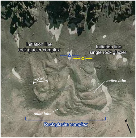
Figure 3. Examples of rock glacier initiation line locations. The yellow circle marks the approximate location of the initiation line of a single talus-derived rock glacier. The blue triangle marks the initiation line location which was actually mapped for this specific rock glacier complex at the head of the Irishman Stream valley, Ben Ohau Range (43.988° S, 170.050° E). Arrows highlight the conspicuously convex morphology of active rock glacier lobes, in contrast to the less distinct, collapsed appearance of older relict lobes further downslope. Image: Orthophotograph 2006 (Terralink, 2004-2010).

We mapped the distribution of talus-derived rock glaciers (including protalus rock glaciers, representing the early stages of permafrost creep; Shakesby, 1997) in the study regions based on a color orthophoto mosaic (Terralink, 2004-2010; pixel size 0.75 m, horizontal accuracy ±3–10 m) and Google Earth imagery available at mid-2010. The landforms were recorded as point features in ArcMap 9.3 (ESRI, 2009a) at the approximate rock glacier initiation line center point (Figure 3). For intricate rock glacier complexes, a single representative point feature was mapped as opposed to multiple features with similar topoclimatic characteristics in proximity to each other. By mapping a single point, we avoided redundant information biasing the statistical evaluation of the relationship between permafrost presence and the topoclimatic variables.

For each rock glacier or rock glacier complex, the present activity state was recorded. Differentiation of active, inactive, and relict features was based on imagery interpretation using commonly recognized visual diagnostics, such as morphology, convexity, appearance of the upper surface, and steepness of the frontal slope (e.g., Barsch, 1996; Ikeda and Matsuoka, 2002; Roer and Nyenhuis, 2007). Spatially compact rock glacier complexes (Figure 3), comprising creep features of differing activity states, were classified in favor of the higher activity class (active or inactive, if applicable). For spatially extensive rock glacier sequences with comparatively small active or inactive landforms nested at the head area of large relict rock glaciers, two point features representing both rock glacier generations (active/inactive and relict) were mapped for completeness.

Differentiation of protalus rock glaciers from landforms with similar morphology, such as pronival ramparts (e.g., Shakesby, 1997), moraines, or landslide deposits, and visual determination of their activity status is often challenging. Therefore, care was taken to only map features where both the appearance of the protalus ridge as well as the landform assemblies of the wider environment suggested a permafrost-related genesis. The probability of present-day ice within the identified protalus rock glaciers was again judged exclusively on visual criteria. Only ramparts of conspicuous convexity were mapped as active. Similarly, tongue-shaped debris-covered features without the characteristic ridge-and-furrow topography (e.g., in the Inland Kaikoura Range, 42.016° S, 173.633° E) were omitted from the inventory due to a possible glacial origin. Geophysical field investigations would be necessary to clarify whether these features are debris-covered glaciers or permafrost creep without significant transpression and buckle folding.

Model Training

We used logistic regression to identify typical MAAT and solar radiation values at the location of active rock glaciers and thus modern permafrost occurrences. The regression model was calculated in SPSS 20 (IBM Corp, 2011); additional model quality measures were computed in ROC-AUC (Schroeder, 2003). Moran's I test for spatial autocorrelation was performed in ArcGIS 9.3 (ESRI, 2009a).

Principles of Logistic Regression

Logistic regression models are generalized linear models that predict the conditional probability for a dichotomous outcome (variable Y) to occur [e.g., permafrost present (1), permafrost absent (0)] based on a set of explanatory variables X (Peng and So, 2002). Since the dichotomous outcome Y can take only one of two values, the relationship between Y and an independent variable X_n is “S-shaped.” Binary values violate the basic assumption of linear regression models that the relationship between predictor and outcome variable is linear. To address this violation, logistic regressions calculate conditional probabilities as the natural logarithm of the odds of Y taking a specific value (referred to as logit or log-odds):

$\begin{array}{ll}ln\left(\frac{P(Y=1)}{1-P(Y=1)}\right)=B_0+B_1{X}_1+B_2{X}_2+\cdots +B_n{X}_n& (1)\end{array}$

where P(Y = 1) is the probability of outcome Y taking the value 1, B₀ the intercept, and B_n the regression coefficient of the explanatory variable X_n. This way, the “form” of the relationship becomes linear while the relationship itself stays non-linear. Solving for P(Y = 1), a multivariate global logistic regression model can thus be described by the equation:

$\begin{array}{ll}P\left(Y=1\right)=\frac{1}{1+e^{-(B_0+{\displaystyle {\sum }_k}{B}_k{X}_k)}}& (2)\end{array}$

where e is the base of the natural logarithm.

Dependent Variable – Active and Relict Rock Glaciers

Active and relict talus-derived rock glaciers (including protalus rock glaciers) were used as a dichotomous dependent variable in the regression model, representing permafrost presence (1) and permafrost absence (0) at the sample locations. Where active rock glaciers occur nested in larger relict rock glaciers, we included only the active rock glaciers in the regression analysis, as both features would be characterized by similar topoclimatic conditions and thus bias statistical relationship analyses.

Although by definition inactive rock glaciers also indicate the presence of permafrost, their utilization for predictive permafrost models is questionable. Firstly, the differentiation of inactive rock glaciers from active or relict features is generally difficult based on visual interpretation of remotely sensed imagery alone and thus inherently associated with high uncertainty (cf. Nyenhuis, 2006). Consequently, in practice, the category “inactive” also comprises ambiguous cases, where visual characteristics do not quite fit either the active or the relict rock glacier description. Secondly, inactivity can be due both to deteriorated climatic conditions or reduced sediment supply (climatic vs. dynamic inactivity, e.g., Barsch, 1996). Differentiation between these two inactivity states is only possible by field assessment of the local temperature regime and debris/ice supply conditions. While climatically inactive rock glaciers might be indicators of permafrost presence, as they still contain—albeit degrading—ice, they are inadequate for characterizing favorable topoclimatic conditions for permafrost presence. For these reasons, inactive rock glaciers were omitted from the regression analysis. This approach is supported by the modeling results of Nyenhuis (2006), who compared the predictive power of permafrost distribution models using different combinations of active, inactive, and relict rock glaciers as input data. Nyenhuis (2006) model based solely on active and relict rock glaciers had the highest predictive power.

Independent Variables – MAAT and Solar Radiation

Spatially-distributed information on MAAT [°C] was modeled for the standard climate period 1971–2000 by spatially interpolating and altitudinally extrapolating daily temperature data from nearby climate stations available in the National Climate Database (NIWA, 2010). Daily temperature data from available stations was (1) lapsed to sea level, using a constant lapse rate of 5°C km⁻¹ [conforming with Norton's (1985) empirical New Zealand-wide average lapse rate; see below] and a 25 m digital elevation model (DEM; Barringer et al., 2002) for elevation information, (2) interpolated between the stations to create a reference surface, and (3) extrapolated to the elevation of each grid point. For computational reasons (large data quantity over large areas), the grid resolution was set to 100 m. This generalization was considered reasonable, given that MAAT only moderately decreases over short distances.

Uncertainty exists in the selection of an appropriate lapse rate for regional temperature modeling in the Southern Alps. Measurements of near-surface lapse rates in the Southern Alps are rare, impeded by the low density of long-term climate stations at elevations of ~1000 m asl and the complete absence of stations at summit height. Existing calculations between lowland and high-altitude observations suggest mean values lower than the standard environmental lapse rate of 6.5°C km⁻¹ (Barry, 2008), but comparable to long-term observations in other mountain ranges (e.g., Rolland, 2003, European Alps, 5.4–5.6°C km⁻¹) and consistent with a cloudy, humid, maritime climate. Norton (1985) calculated a mean annual lapse rate of 5°C km⁻¹ from temperature data (1950–1980) from 301 New Zealand climate stations. Similar values were reported from short-term measurements at the Franz Josef Glacier by Anderson et al. (2006, 5°C km⁻¹) and for the Ben Ohau Range by Doughty (2013, 5.4°C km⁻¹), although the latter noted that the annual mean was influenced by large seasonal variability, especially winter temperature inversions. Tait's (2010) comparison of different temperature interpolation methods for the Southern Alps supports the use of the 5°C km⁻¹ gradient for regional-scale distributed MAAT modeling. Based on these observational studies, we consider the use of a lapse rate of 5°C km⁻¹ reasonable for the present study.

Spatially-distributed solar radiation [kWh m⁻²] was calculated in ArcGIS 9.3 (ESRI, 2009a) using the “Area Solar Radiation” tool and a 15 m DEM (Columbus et al., 2011). The underlying model accounts for both DEM tiles' latitude as well as local viewshed and thus enables the identification of variations in insolation on catchment scale. Information on the tool itself and employed algorithms are published in Fu and Rich (2000) and the ArcGIS online resources (ESRI, 2009b). Insolation sums were calculated for the snow-free period December to May (inferred from ground surface temperature observations in the Ben Ohau Range, see below), since incoming shortwave radiation influences subsurface temperatures only in times of low albedo, i.e., when the ground is not covered by a reflective and insulating snow cover (e.g., Hoelzle, 1994). Due to lack of meteorological field data, default values representing general clear sky conditions were used as radiation parameter inputs (uniform diffuse radiation model, diffuse proportion 0.3, and transmittivity 0.5). The grid resolution was kept at 15 m to acknowledge the high spatial variability of insolation in mountain areas.

Model Evaluation

The modeled permafrost extent was evaluated by winter equilibrium temperatures at the snowpack base derived from continuous ground surface measurements using miniature data loggers in the head area of Irishman Stream valley, central Ben Ohau Range (Figure 1). The Irishman Stream valley was selected as an evaluation site based on the presence of extensive high-altitude debris slopes of all orientations, as well as the presence of active rock glaciers indicating that the area intersects the permafrost zone.

The use of winter equilibrium temperatures derived from data loggers as a permafrost indicator builds on Haeberli's (1973) bottom temperature of the winter snow cover (BTS) method for permafrost mapping. Both methods are based on the low thermal conductivity of a sufficiently thick snow cover (>80–100 cm), which insulates the subsurface from air temperature variations during the winter months (e.g., Haeberli, 1973; Brenning et al., 2005). During that time, temperatures at the snowpack base, i.e., ground surface temperatures, are mainly controlled by heat transfer from below and thus they are influenced by the presence or absence of permafrost. Ground surface temperatures above permafrost have been observed to reach an equilibrium toward the end of the winter season (i.e., before the onset of the snow melt) generally below −3°C (e.g., Haeberli, 1973, 1978; King, 1983). At locations without permafrost, surface temperatures commonly leveled out above −2°C. From these observations, the BTS interpretation guidelines were derived (Hoelzle, 1992), where temperatures below −3°C indicate probable permafrost presence, temperatures between −2 and −3°C possible permafrost presence, and temperatures above −2°C improbable permafrost presence. BTS measurements are traditionally conducted in late-winter field campaigns, using long thermistor probes to assess winter equilibrium temperatures at the snowpack base (e.g., Lewkowicz and Ednie, 2004). More recently, winter equilibrium temperatures are increasingly inferred from continuous ground surface temperature measurements by data loggers (e.g., Hoelzle et al., 2003; Schöner et al., 2012). The continuous recordings allow the evaluation of the ground surface temperature development throughout the winter season and thus enable an informed judgment on the reliability of inferred winter equilibrium temperatures. The empirical temperature interpretation thresholds have to be considered only indicative as winter equilibrium temperatures vary interannually due to snow cover history (e.g., Imhof et al., 2000; Hoelzle et al., 2003; Brenning et al., 2005) and can be modified by local factors such as air advection processes (e.g., Lambiel and Pieracci, 2008). However, BTS and winter equilibrium temperatures derived from continuous measurements have been successfully applied in many mountainous regions for permafrost investigations (e.g., Swiss Alps: Hoelzle, 1992; Southern Norway: Isaksen et al., 2002; Yukon Territory, Canada: Lewkowicz and Ednie, 2004; Austrian Alps: Schöner et al., 2012; Southern Carpathians, Romania: Onaca et al., 2013).

We inferred winter equilibrium temperatures from 23-month continuous ground surface temperature measurements by HOBO^® Pendant Temperature/Light Data Loggers (UA-002-08; 0.5°C accuracy and 0.1°C resolution at 0°C) at 44 sites at the head of the Irishman Stream valley. A preliminary permafrost distribution estimate, derived from the mean toe elevation of intact rock glaciers mapped in the Ben Ohau Range, was used to identify suitable monitoring sites. Thirty-four data loggers were distributed in longitudinal profiles on slopes of eight aspect classes, another seven placed in different surface cover types along the valley floor, and three loggers installed on active rock glaciers to exemplify the annual ground surface temperature evolution above permafrost occurrences. Winter equilibrium temperature was calculated as the mean ground surface temperature of the first fortnight (1st–14th) of September, a period when, at most monitoring sites in both winter seasons, the ground surface temperature was steady before the onset of snow melt.

The use of continuous ground surface temperature recordings for winter equilibrium temperature assessment was vital for the present study, as neither BTS nor continuous temperature measurements had previously been tested for permafrost mapping in the Southern Alps. A primary concern was that the intermittent melt periods characteristic of New Zealand's alpine winter conditions might not adequately decouple the subsurface from atmospheric influences. Consequently, ground surface temperature would not reach an end-of-winter equilibrium. This behavior has been observed in Iceland (Etzelmueller et al., 2007), preventing the use of BTS or data logger derived winter equilibrium temperatures for permafrost prospecting in the Icelandic mountains.

Results

Rock Glacier Inventory

Overall, 382 talus-derived rock glaciers were mapped in the central Southern Alps and the Inland Kaikoura Range (Figure 4; see Supplementary Material for inventory in tabular form). The majority (88%) of the rock glaciers (or rock glacier complexes) were well-developed with one or more distinct lobes. The remaining 12% of the mapped features were interpreted as protalus rock glaciers. Almost a fifth of all rock glaciers (19%) were thought to be active; a quarter (23%) were interpreted as inactive. The majority (58%) of the mapped rock glaciers were classified as relict features that no longer contain ice.

FIGURE 4

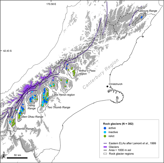
Figure 4. Rock glacier inventory for the Canterbury Region, separated into seven topographic regions. The western (and equally upper altitudinal) boundary of rock glacier occurrence in the Canterbury Southern Alps corresponds well with Lamont et al.'s (1999) equilibrium line altitude (ELA) estimates of 2000–2200 m for the eastern ranges. Glacier extent: Randolph Glacier Inventory 5.0 (GLIMS/NSDIR, 2015), elevation data: 25 m DEM, Barringer et al. (2002), coastline and regional boundaries: Statistics New Zealand (2013).

The distribution of rock glaciers in the Southern Alps conforms with the temperature- and precipitation constrained distribution patterns commonly described in the literature (e.g., Haeberli, 1985; Barsch, 1996; Humlum, 1998). Rock glacier occurrence in the Southern Alps is characterized by a distinct western boundary ~20 km east of the Main Divide (Figure 4). This boundary corresponds well with Lamont et al.'s (1999) estimates of glacial equilibrium line altitudes of 2000–2200 m asl in the eastern ranges, supporting the general assumption that talus rock glaciers predominantly occur in cold areas too dry for glacier maintenance. The temperature constraint on rock glacier distribution is evident when plotting the rock glacier initiation line altitude of active and relict features against rock glacier orientation (Figure 5A), demonstrating a vertical trend with active rock glaciers occurring at higher elevations than relict rock glaciers. The scatterplot further confirms an aspect dependence, with active features occurring at higher elevations in northern, sun-facing orientations. The observed variations in the location of active and relict rock glacier sites according to altitude and aspect support the use of the underlying environmental controls MAAT and solar radiation for predictive permafrost modeling at catchment scale. Furthermore, the selected modeling approaches for MAAT and solar radiation appear adequate, as the altitude- and aspect-dependency in the distribution of active and relict features is reproduced when plotting the estimated MAAT at the rock glacier initiation line against solar radiation (Figure 5B). Both active and relict features are more numerous at locations with comparatively low insolation totals, but active rock glaciers exist at colder temperatures, highlighting temperature as the influential discriminating factor between permafrost presence and absence at rock glacier sites.

FIGURE 5

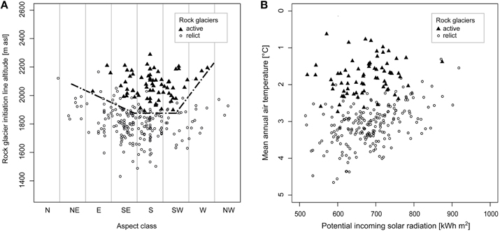
Figure 5. Differences between active and relict rock glaciers in initiation line altitude and orientation (A) and mean annual air temperature and potential incoming solar radiation in snowfree months (B).

Regression Model

Statistical analysis was based on a dataset of 71 active and 209 relict rock glaciers and their respective topoclimatic attributes. The three active rock glaciers mapped in the Inland Kaikoura Range (see Figure 4) were omitted from the analyses to avoid potential bias of the regression results. In this region no relict features were mapped and inclusion of the region would unduly influence comparison of permafrost favorable and unfavorable topoclimatic conditions.

The regression model's overall fit as well as all coefficient estimates were highly significant (bootstrap p < 0.001, Table 1). The results indicate that MAAT and solar radiation adequately predict the presence of active rock glaciers. Multicollinearity statistics (variance inflation factor) indicate the absence of correlation between the predictor variables biasing the coefficient estimates. Moran's I analysis showed regression residuals are spatially independent (Moran's I = 0.059, p = 0.507) and parameter estimates thus unbiased by spatial autocorrelation of observations. As expected, both MAAT and solar radiation are negatively related to permafrost occurrence. In other words, the lower both MAAT and solar radiation at the rock glacier initiation line, the higher the probability that the mapped feature is still active. Recalculation of the regression model with standardized predictor variables confirms MAAT as the more influential discriminating factor between permafrost presence and absence at rock glacier sites (cf. Section Rock Glacier Inventory) with MAAT (B_Z = −5.286, p < 0.001) having a more than three times larger effect on the calculated permafrost probability than solar radiation (B_Z = −1.556, p < 0.001).

TABLE 1

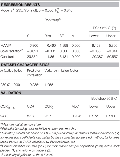
Table 1. Logistic regression output, dataset characteristics, and validation statistics.

Validation criteria suggest that the regression model achieves a high predictive accuracy (Table 1). The area under the curve (AUC) score of 0.984 indicates an excellent discriminative ability between permafrost presence and absence (Hosmer and Lemeshow, 2000). This is also shown by the high overall correct classification rate (CCR_TOTAL) of 94.3%, assuming the common cutoff value of 0.5. However, the difference between correctly classified presence (CCR₁ = 87.3%) and correctly classified absence (CCR₀ = 96.7%) signals that the model performs better at predicting permafrost absence than permafrost presence.

Permafrost Distribution in the Southern Alps

Spatially-distributed conditional probabilities of permafrost presence were computed in ArcMap 9.3 with raster calculator, inserting the regression's coefficient estimates (Table 1) in Equation (2). A probability threshold of 0.6 was chosen to discriminate between “permafrost probable” (P ≥ 0.6) and “permafrost improbable” (P < 0.6) locations and thus for delineating the potential permafrost extent. This classification cutoff is slightly more conservative than values used in other probability-based permafrost distribution estimates (e.g., Lewkowicz and Ednie, 2004; Janke, 2005; Ridefelt et al., 2008), but coincides with the optimal cutoff of 0.598, calculated with the software program ROC-AUC (Schroeder, 2003) as the threshold at which the regression model achieves maximum correct classification rates (CCR_TOTAL = 94.6%) for the analyzed rock glacier inventory.

For a general altitudinal characterization of the potential permafrost extent in the Southern Alps, the predictive model was applied to the seven regions of rock glacier occurrence (Figure 6), signifying the areas of highest reliability of the developed model given the presence of permafrost indicators. Frequency analysis of the calculated probabilities revealed that topoclimatic conditions were, in the majority of locations, either highly favorable for permafrost occurrence (P ≥ 0.9) or not favorable (P < 0.6). The lack of notable spatial transition zones between these probability classes (Figure 6C) arises from pronounced vertical changes in MAAT (i.e., the dominant predictor) in the generally steep terrain of permafrost favorable areas in the Southern Alps. Likelihood values of 0.6–0.7 were particularly rare, occurring largely as a thin spatial band around the lower rim of the modeled permafrost extent (cf. Figure 6C). Their confined spatial distribution allows the inference of mean lower limits of the modeled permafrost distribution (Table 2). In the central ranges of the Southern Alps, permafrost is probable above 1866 m asl on south-facing slopes and above 2120 m asl on north-facing slopes; the average lower boundary of permafrost occurrence lies at 2000 m asl. In the Inland Kaikoura Range, the calculated limits are higher: Permafrost is probable above 2062 m asl on south-facing slopes and above 2261 m asl on north-facing slopes with a mean lower limit of 2148 m asl.

FIGURE 6

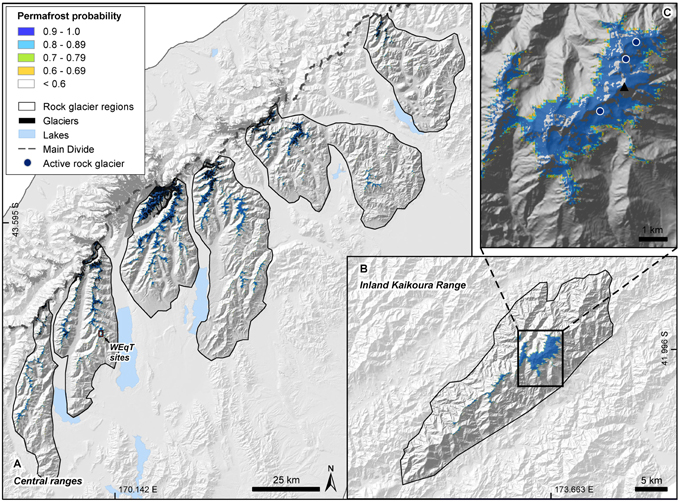
Figure 6. Permafrost probability distribution in the central rock glacier regions (A), the Inland Kaikoura Range (B), and the Tapuae-o-Uenuku (▴) area (C). In panel (A), the rectangle signifies the location of the winter equilibrium temperature (WEqT) measurement sites. In panel (C), rock faces are masked by removing areas with a gradient ≥ 40° from the probability layer. Glacier extent: Randolph Glacier Inventory 5.0 (GLIMS/NSIDR, 2015), background: hillshade of 25 m DEM, Barringer et al. (2002).

TABLE 2

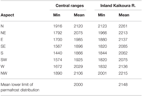
Table 2. Elevation summary [m asl] for locations with permafrost probability between 0.6 and 0.7 according to aspect classes as well as averaged over all orientations, representing the estimated lower limit of the potential permafrost extent in the central Southern Alps and the Inland Kaikoura Range.

Comparison with Winter Equilibrium Temperatures

The 2-year ground surface temperature records revealed a high interannual variability in (1) the distribution of sites with ground surface temperature profiles suitable for winter equilibrium temperature interpretation, and (2) inferred winter equilibrium temperatures (Figures 7A,B). A stable winter equilibrium temperature developed each year at roughly a third of the monitoring sites; however, the distribution of these sites differed significantly between the years. Inferred winter equilibrium temperatures for 2011 indicated generally colder temperatures than the previous winter. The lower temperatures likely resulted from a later onset of snow insulation in 2011 (Figure 8).

FIGURE 7

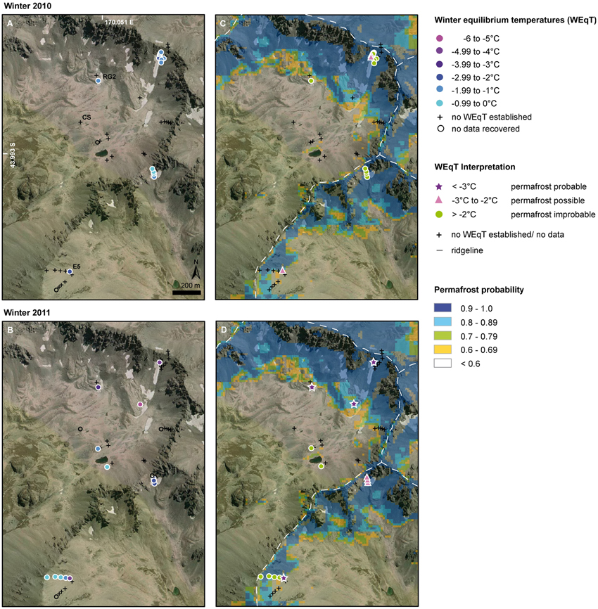
Figure 7. Winter equilibrium temperature (WEqT; A,B) and inferred permafrost probability (C,D) at the ground surface temperature monitoring sites in the Irishman Stream area for winter 2010 and 2011. In panel (C,D), rock faces are masked by removing areas with a gradient ≥ 40° from the modeled permafrost extent. The modeled permafrost extent matches the WEqT-indicated permafrost sites well, suggesting a reasonable model output. Basemap: Orthophotograph 2006 (Terralink, 2004-2010).

FIGURE 8

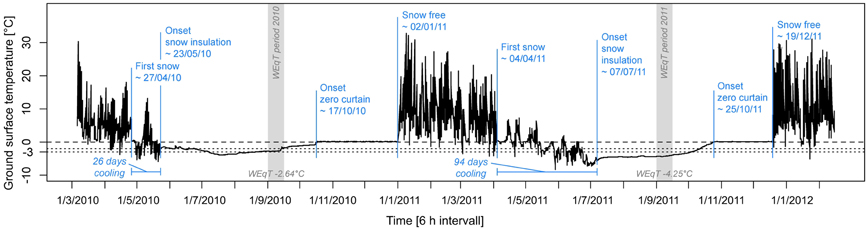
Figure 8. Twenty-three month record of ground surface temperature development at site E5 (for location see Figure 7A), illustrating the influence of snow cover conditions in early winter on winter equilibrium temperatures (WEqT). Gray vertical bars signify the WEqT measurement periods; calculated WEqT are given at the bottom of the bars.

Brenning et al. (2005) consider years with thermal regimes affected by early snow cover development better suited for winter equilibrium temperature interpretations than those characterized by significant ground cooling prior to the development of an insulating snow cover. However, given that the former is likely to produce warmer temperatures than the “true” equilibrium temperature, Brenning et al. (2005) recommend adjusting inferred winter equilibrium temperatures according to mean deviations from the long term average characteristic for the respective thermal regime. Such corrective measures were not possible in the present study given the short period of ground surface temperature records. Instead, the winter equilibrium temperatures for the two seasons are interpreted as describing two “end member” distribution patterns, with the warmer 2010 temperatures representing conservative estimates of permafrost presence at the investigation sites and the colder 2011 values illustrating a more liberal approximation.

Overall, the modeled permafrost extent reasonably matches the winter equilibrium temperature-indicated permafrost sites (Figures 7C,D). The strong aspect control on permafrost occurrence suggested by the model for the validation area is supported by the distribution of the possible and probable permafrost sites. Winter equilibrium temperatures from 2011, which might be biased toward lower temperatures, did not indicate permafrost occurrences outside the modeled extent. However, only a few sites below the modeled extent showed ground surface temperature development suited for winter equilibrium temperature interpretation that year. The potential permafrost extent according to the liberal winter equilibrium temperature scenario is therefore untested. The winter equilibrium temperature-indicated permafrost presence at the frontal lobe of the western rock glacier (“RG2” in Figure 7A) forms an exception in this context. The permafrost model was purposely based on topoclimatic conditions at the head of active rock glaciers to avoid overestimating the potential permafrost extent due to the mobility of rock glaciers and their ability to preserve permafrost even in topoclimatically hostile locations. The presence of an active rock glacier extending beyond the modeled lower distribution limit therefore supports the idea that the model provides a conservative estimate of the permafrost distribution. Likewise, winter equilibrium temperature measurements suggesting the absence of permafrost at locations for which high permafrost probabilities were predicted do not falsify the model results. These deviations are rather an expression of the high local variability of permafrost (e.g., Lambiel and Pieracci, 2008), which in reality is strongly influenced by thermal properties of the surface and subsurface material, aspects that were not considered in our low-order catchment-scale distribution estimate.

Discussion

Use and Limitations of the Model

Our model demarks potential permafrost areas in the Southern Alps at catchment scale (e.g., Figure 6) and characterizes lower permafrost distribution limits in this maritime setting (Table 2). Based on a spatially extensive rock glacier inventory that covers a significant proportion of the mountain chain's high-altitude areas, the model is likely applicable in all of the Southern Alps. However, as rock glaciers belong to the debris domain, inferred conditional probabilities are strictly-speaking only valid for evaluating permafrost occurrences in debris-mantled slopes. The combination of our model with an extended, regionally-applicable version of Allen et al.'s (2009) bedrock permafrost distribution model would provide a complete debris-bedrock permafrost estimate for the Southern Alps, similar to Boeckli et al.'s (2012) model for the European Alps.

The largest uncertainty in our model results from the use of a spatially-uniform lapse rate for temperature extrapolations. Although observational studies in the Southern Alps support the use of a 5°C km⁻¹ lapse rate for regional temperature modeling (cf. Section Independent Variables – MAAT and Solar Radiation), it is nonetheless well-known that near-surface lapse rates vary both in time (e.g., Rolland, 2003; Doughty, 2013) and space (e.g., Pepin et al., 1999; Minder et al., 2010). Allen et al. (2009) calculated a mean annual lapse rate of 6°C km⁻¹ close to the Southern Alp's Main Divide and 7°C km⁻¹ for a drier location 10 km further east from 12-month records of two high-altitude station pairs. Their results indicate significant changes in lapse rates over short distances, presumably corresponding to the region's strong gradients in humidity-related parameters such as rainfall and cloud cover. However, translation of these observations into regional-scale estimates of surface lapse rates, suitable for utilization in our model, would require a more extended set of measurements over a larger area (cf. Minder et al., 2010). Calculations would further need to take into account seasonal and interannual variability in climate resulting from the influence of, for instance, the El Niño Southern Oscillation and Southern Annular Mode. Both would be challenging, given the low density of suitable climate observations in the Southern Alps; more high-elevation stations are urgently needed.

Comparison to Other Permafrost Distribution Studies

Our results indicate that climatic conditions are favorable for permafrost occurrence above ~2000 m asl (± ~100 m) in the central Southern Alps (Table 2). This finding fits well with previous estimates by Brazier et al. (1998) and Gorbunov (1978) which were derived by different means. The higher altitudinal limit of 2148 m asl (± ~70 m) calculated for the Inland Kaikoura Range represents the shift of suitably cold climatic condition to higher elevations at the warmer top of the South Island, conforming with the global trend of increasing elevational permafrost limits with decreasing latitude (e.g., Cheng and Dramis, 1992).

This latitudinal trend is also evident when comparing the altitudinal distribution of the Southern Alps' rock glacier inventory to that of other published datasets (Figure 9). For example, the mean rock glacier initiation line altitude of active rock glaciers in New Zealand is lower than in the Nepal Himalaya (Regmi, 2008), but higher than in Canada (Page, 2009) or Alaska (Wahrhaftig and Cox, 1959). Interestingly, both rock glacier-related and modeled altitudinal limits (Figure 9) are significantly lower in the maritime Southern Alps than in the continental European Alps (Haeberli, 1975, 1996; Schrott et al., 2012) despite being located at comparable latitudes. Similar deviations are evident for estimated permafrost limits in the Japanese mountains (Matsuoka, 2003) and rock glacier occurrence in the Antarctic South Shetland Islands (Serrano and López-Martıìnez, 2000), all situated within 100 km of the coast. The deviations are also present, but less pronounced in the Yukon dataset (Page, 2009) with active rock glaciers in the Kluane Ranges occurring at lower altitude than in the ~480 km further inland situated Bonnet Plume Range.

FIGURE 9

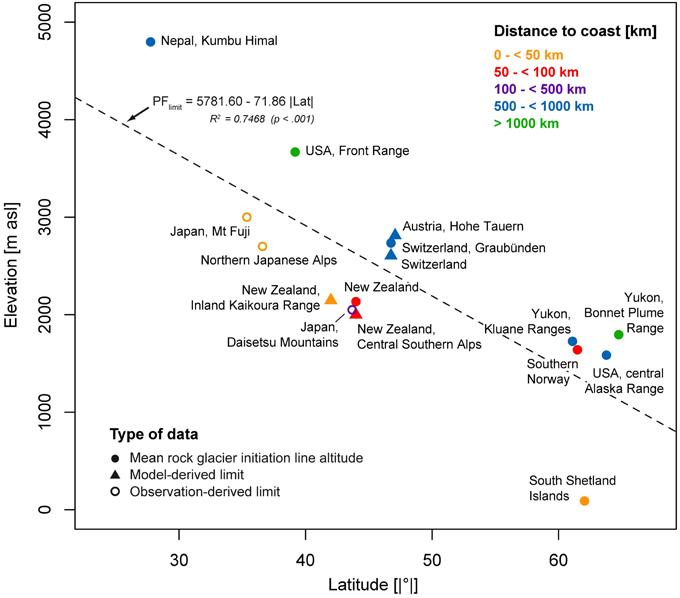
Figure 9. Comparison of the Southern Alps' lower permafrost distribution limits to data from selected other temperate climate regions according to distance to sea. Full circles (•) represent limits derived from the mean rock glacier initiation line altitude of active features; sources: Nepal, Kumbu Himal, Regmi (2008); USA, Front Range, Janke (2007); Switzerland, Graubünden, Haeberli (1975); Canada, Yukon, Page (2009); Southern Norway (active and inactive rock glaciers), Lilleøren and Etzelmüller (2011); USA, central Alaska Range, Wahrhaftig and Cox (1959); South Shetland Islands, Serrano and López-Martıìnez (2000). Full triangles (▴) represent limits derived from distribution models; sources: Austria, Hohe Tauern (steep slopes, probable permafrost limit), Schrott et al. (2012); Switzerland (steep slopes, possible permafrost limit), Haeberli (1996). Empty circles (◦) represent limits derived from permafrost observations in the Japanese Alps, published in Matsuoka (2003). Dashed line represents the dataset's average polewards decrease in permafrost limits of 72 m per degree latitude.

These differences suggest the presence of an oceanic control on global permafrost distribution limits in addition to the well-acknowledged latitudinal control. A possible influence is the effect of moderate annual temperature amplitudes, characteristic for maritime climates (cf. Sturman and Wanner, 2001, see also Figure 2), on the preservation of permafrost. Low summer maxima may significantly reduce ground warming and ice loss during the warm seasons (cf. Brazier et al., 1998), facilitating the existence of permanently frozen ground at lower altitudes. Establishing the underlying climatic controls would require physical models that include all energy fluxes above maritime permafrost occurrences (e.g., Luetschg et al., 2008; Staub et al., 2015). Such energy balance studies, accompanied by long-term ground temperature, surface temperature, and snow cover monitoring, would further allow exploring the effect of maritime snow conditions on long-term subsurface temperature evolution. A frequent occurrence of significant subsurface cooling before snow cover onset, as observed at the winter equilibrium temperature monitoring sites in 2011 (Figure 8) but also common in other mountain ranges (cf. Brenning et al., 2005), may counteract the efficient insulation by thick maritime snow packs, seen by Gruber and Haeberli (2009) as the limiting factor of perennially frozen debris in maritime settings.

A lower than expected limit of permafrost extent in the Southern Alps is also suggested by the comparison of Gruber's (2012) permafrost zonation index map for the Southern Alps and our distribution estimate (Figure 10). Our model results are in good agreement with Gruber's “fringe of uncertainty” extent, which represents a “more conservative than normal” scenario that considers the possibility of <10% permafrost area also where MAAT is positive. Our estimate is more refined, since it is based on the regression of Southern Alps field observations. Hence it appears that the cold variant assumption is more appropriate for the application of Gruber's (2012) model in New Zealand than its normal assumption. Comparison of the global permafrost zonation index maps to distributed permafrost models in other maritime mountain ranges might reveal a systematic underestimate of the permafrost extent in maritime settings by Gruber's (2012) model. Such a finding would lend further support to the idea that permafrost generally occurs at lower elevations in maritime settings.

FIGURE 10

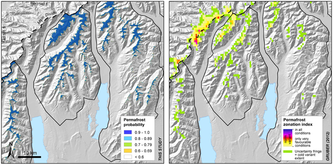
Figure 10. Comparison of this study's model results and Gruber's (2012) global permafrost zonation index for the Liebig Range and Two Thumb Range, central Southern Alps. The results indicate that Gruber's cold variant assumption may be more appropriate for the application of Gruber's (2012) model in New Zealand than its normal assumption. Background: hillshade of 15 m DEM, Columbus et al. (2011).

Positive MAAT at Active Rock Glacier Sites in the Southern Alps

Based on our temperature interpolations, utilizing a spatially uniform lapse rate of 5°C km⁻¹, the head area of all active rock glaciers in the Southern Alps are situated below the mean annual 0°C-isotherm (range 0.3–2.7°C, median 1.8°C; cf. Figure 5B). Active rock glaciers in locations with positive MAAT have been occasionally reported from the Andes (Trombotto et al., 1997; Brenning, 2005), and from the maritime Falkland Islands (Birnie and Thom, 1982) and Iceland (Eyles, 1978). However, such observations are unusual by global standards (cf. Barsch, 1996; Humlum, 1998; Frauenfelder et al., 2003; Janke and Frauenfelder, 2008).

The positive MAAT at the Southern Alps' rock glacier sites may indicate that the lapse rate of 5°C km⁻¹ used in this study is inappropriately low. For example, application of Allen et al.'s (2009) steeper lapse rates would place the mapped rock glaciers in the negative MAAT range associated with permafrost limits in other mountain regions, as illustrated by Brazier et al. (1998) for active rock glaciers in the Ben Ohau Range. However, several independent temperature datasets suggest that the modeled positive temperatures might not be unrealistic. MAAT interpolations underlying Gruber's (2012) model also indicate relatively warm temperatures at the mapped active rock glacier sites (range −1.4−2.8°C, median −0.1°C). Similarly, extrapolating MAAT observed at the short-term climate station in the Irishman Stream valley (“CS” in Figure 7A) to the rock glacier initiation lines of the two nearby rock glaciers, using Doughty's (2013) lapse rate of 5.4°C km⁻¹ derived from this station, indicated positive temperatures (1.5 and 1.8°C, respectively). Lastly, extrapolating MAAT derived from the global WorldClim temperature dataset (Hijmans et al., 2005; 30 arc-seconds resolution, 1950–2000 temperature normals) to permafrost limits at the international permafrost sites, using the standard environmental lapse rate of 6.5° km⁻¹ (Barry, 2008) and WorldClim's elevation dataset, suggests positive MAAT for New Zealand permafrost occurrences (Figure 11). Calculated temperature normals for the international permafrost sites are associated with high uncertainty, given the arbitrary placement of sample locations at the approximate center of the documented permafrost regions, averaging of climatic parameters within a 2 km radius to increase the regional representativeness of the point-derived information, and the use of a global lapse rate irrespective of local observations. Nonetheless, plotting the mean annual temperature range as a measure for continentality, calculated as the difference between WorldClim's mean temperatures of the coldest and warmest month, against MAAT at mean rock glacier initiation line altitudes and estimated lower permafrost limits suggests the presence of a global trend of increasing MAAT with increasing oceanity (Figure 11). The New Zealand datasets fit the indicated trend by showing the highest MAAT as the least continental location of the international permafrost sites.

FIGURE 11

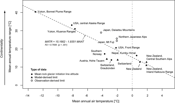
Figure 11. Comparison of mean annual temperature range (MATR) and mean annual air temperature (MAAT) at mean rock glacier initiation line altitudes and estimated permafrost limits of the international permafrost sites. The comparison suggests the presence of a global trend of increasing MAAT at permafrost sites with decreasing continentality.

Applicability of Winter Equilibrium Temperatures for Permafrost Prospecting in New Zealand

Our ground surface temperature records suggest that winter equilibrium temperatures can potentially be used for permafrost prospecting in the Southern Alps. At approximately a third of the monitoring sites each year, snow pack conditions (height, wetness) were suitable for the development of winter equilibrium temperatures. However, our records demonstrated high interannual variations in both the distribution of sites with ground surface temperature profiles suited for winter equilibrium temperature interpretation and inferred winter equilibrium temperatures. Related to typically strong year-to-year variations in snow distribution as well as the timing of snow pack development, this variability has been identified as a critical limitation of winter equilibrium temperature interpretations in the past (e.g., Hoelzle et al., 2003; Brenning et al., 2005). Future studies in the Southern Alps should therefore be conducted by continuous data loggers to allow evaluation of the inferred winter equilibrium temperatures' reliability. Furthermore, winter equilibrium temperature interpretation thresholds should be tested using geophysical methods. Our attempts to verify permafrost presence at the monitoring sites by electrical resistivity tomography measurements (16 electrode GF Instruments Automatic Resistivity System, 5 m electrode spacing, various array configurations tested) during two field seasons were unsuccessful, most likely due to a combination of dry ground conditions toward the end of the summer and insufficient coupling between large blocks and electrodes at the talus footslopes. Improved resistivity measurement set-ups, utilizing water-saturated sponges in steel nets (e.g., Ishikawa, 2008) or the placement of electrodes into small holes drilled into rock (e.g., Kneisel and Hauck, 2008), might allow to overcome the technical challenges encountered in this study.

Systematic multi-scale sampling strategies, such as recently presented by Gubler et al. (2011), could provide large datasets of continuous ground surface temperature profiles allowing a scale-dependent analysis of winter equilibrium temperatures and their spatial variations. These datasets would represent a valuable addition to the limited number of rock glaciers currently available for the investigation of permafrost occurrence and distribution in the Southern Alps.

Conclusion

Our catchment-scale permafrost model provides a first-order estimate of permafrost distribution in debris-mantled slopes in the Southern Alps of New Zealand, demonstrating the characteristics of permafrost occurrences in a maritime setting. We derived the permafrost distribution model by regression of active and relict rock glaciers against MAAT and potential incoming solar radiation and evaluated the results against winter equilibrium temperature observations.

Our model results suggest that permafrost occurrence is likely above ~2000 m asl in the central Southern Alps and above ~2150 m asl in the Inland Kaikoura Range. The increase in lower distribution limits toward the warmer north of the Southern Alps reflects the global distribution trend of increasing altitudinal limits with decreasing latitude. However, an international comparison of rock glacier altitudes and modeled distribution limits in temperate mountain ranges suggests that distribution limits in the Southern Alps are unusually low. Reduced ice-loss due to moderate summer temperature extremes, characteristic for maritime climate, may facilitate the occurrence of permafrost at lower altitudes than, for example, in the continental European Alps at similar latitude. Empirical rules for permafrost occurrence derived in continental climates may consequently not be applicable in mountain ranges in proximity to oceans. We encourage further research to characterize the related climatic controls.

Author Contributions

KS led the design of the project, mapped the rock glacier inventory, developed the permafrost distribution model, created and interpreted the evaluation datasets, and prepared the manuscript. BA contributed to project design, carried out the MAAT interpolations, assisted with field work, interpretation and writing. AM was KS's primary PhD supervisor and assisted with project design, fieldwork, interpretation and writing. KN and MR assisted with project design, interpretation and writing.

Funding

This project was part of KS's PhD research, funded by a Vice Chancellor's Strategic Research PhD Scholarship, Victoria University Wellington, and by contributions toward fieldwork from the New Zealand Department of Conservation (Inv 4150), Environment Canterbury, and A. Mackintosh.

Conflict of Interest Statement

The authors declare that the research was conducted in the absence of any commercial or financial relationships that could be construed as a potential conflict of interest.

Supplementary Material

The Supplementary Material for this article can be found online at: https://www.frontiersin.org/article/10.3389/feart.2016.00004

References

Allen, S., Owens, I., and Huggel, C. (2008). “A first estimate of mountain permafrost distribution in the mount cook region of New Zealand's Southern Alps,” in Ninth International Conference on Permafrost, eds D. L. Kane and K. M. Hinkel (Fairbanks, AK: Institute of Northern Engineering, University of Alaska), 37–42.

Allen, S. K., Gruber, S., and Owens, I. F. (2009). Exploring steep bedrock permafrost and its relationship with recent slope failures in the Southern Alps of New Zealand. Permafrost Periglac. Process. 20, 345–356. doi: 10.1002/ppp.658

CrossRef Full Text | Google Scholar

Anderson, B., Lawson, W., Owens, I., and Goodsell, B. (2006). Past and future mass balance of 'Ka Roimata o Hine Hukatere' Franz Josef Glacier, New Zealand. J. Glaciol. 52, 597–607. doi: 10.3189/172756506781828449

CrossRef Full Text | Google Scholar

Augustinus, P. (2002). Periglacial research in New Zealand: a review. S. Afr. J. Sci. 98, 64–70.

Google Scholar

Barrell, D. J. A., Andersen, B. G., and Denton, G. H. (2011). Glacial Geomorphology of the Central South Island, New Zealand. GNS Science Monograph, Nr. 27. Lower Hutt: GNS Science.

Barringer, J. R. F., Pairman, D., and McNeill, S. J. (2002). Development of a High-Resolution Digital Elevation Model for New Zealand. Contract Report LC0102/170. Lincoln, OR: Landcare Research.

Barry, R. G. (2008). Mountain Weather and Climate. Cambridge: Cambridge University Press.

Google Scholar

Barsch, D. (1978). “Rock glaciers as indicators of discontinuous Alpine permafrost. An example from Swiss Alps,” in Third International Conference on Permafrost (Ottawa, ON: National Research Council of Canada), 349–352.

Barsch, D. (1996). Rockglaciers - Indicators for the Present and Former Geoecology in High Mountain Environments. Berlin: Springer-Verlag.

Google Scholar

Birnie, R. V., and Thom, G. (1982). Preliminary observations on two rock glaciers in South Georgia, Falkland Islands Dependencies. J. Glaciol. 28, 377–386.

Google Scholar

Boeckli, L., Brenning, A., Gruber, S., and Noetzli, J. (2012). A statistical approach to modelling permafrost distribution in the European Alps or similar mountain ranges. Cryosphere 6, 125–140. doi: 10.5194/tc-6-125-2012

PubMed Abstract | CrossRef Full Text | Google Scholar

Brazier, V., Kirkbride, M. P., and Owens, I. F. (1998). The relationship between climate and rock glacier distribution in the Ben Ohau Range, New Zealand. Geogr. Ann. Ser. A 80A, 193–207. doi: 10.1111/j.0435-3676.1998.00037.x

CrossRef Full Text | Google Scholar

Brenning, A. (2005). Geomorphological, hydrological and climatic significance of rock glaciers in the Andes of Central Chile (33–35°S). Permafrost Periglac. Process. 16, 231–240. doi: 10.1002/ppp.528

CrossRef Full Text | Google Scholar

Brenning, A., Gruber, S., and Hoelzle, M. (2005). Sampling and statistical analyses of BTS measurements. Permafrost Periglac. Process. 16, 383–393. doi: 10.1002/ppp.541

CrossRef Full Text | Google Scholar

Cheng, G. (1983). “Vertical and horizontal zonation of high-altitude permafrost,” in Fourth International Conference on Permafrost, ed T. L. Péwé (Washington, DC: National Academy Press), 139–144.

Cheng, G., and Dramis, F. (1992). Distribution of mountain permafrost and climate. Permafrost Periglac. Process. 3, 83–91. doi: 10.1002/ppp.3430030205

CrossRef Full Text | Google Scholar

Chinn, T. (1995). Glacier fluctuations in the Southern Alps of New Zealand determined from snowline elevations. Arct. Alp. Res. 27, 187–198. doi: 10.2307/1551901

CrossRef Full Text | Google Scholar

Columbus, J., Sirguey, P., and Tenzer, R. (2011). 15m DEM for New Zealand. Available online at: https://koordinates.com (Accessed August 10, 2015).

Doughty, A. M. (2013). Inferring Past Climate from Moraine Evidence Using Glacier Modelling. Unpublished Ph.D. thesis, Victoria University of Wellington, New Zealand.

Google Scholar

ESRI (2009a). ArcGIS 9.3.1 for Desktop. Redlands, CA: Environmental Systems Research Institute.

ESRI (2009b). ArcGIS Desktop 9.3 Help. Available online at: http://webhelp.esri.com/arcgisdesktop/9.3/index.cfm?TopicName=Understanding_solar_radiation_analysis (Accessed August 10, 2015).

Etzelmueller, B., Farbrot, H., Gudmundsson, A., Humlum, O., Tveito, O. E., and Björnsson, H. (2007). The regional distribution of mountain permafrost in Iceland. Permafrost Periglac. Process. 18, 185–199. doi: 10.1002/ppp.583

CrossRef Full Text | Google Scholar

Eyles, N. (1978). Rock glaciers in Esjufjöll Nunatak area, south-east Iceland. Joekull 28, 53–60.

Frauenfelder, R., Haeberli, W., and Hoelzle, M. (2003). “Rockglacier occurrence and related terrain parameters in a study area of the Eastern Swiss Alps,” in Eighth International Conference on Permafrost, eds M. Phillips, S. M. Springman, and L. U. Arenson (Zürich: A.A. Balkeman), 253–258.

Frehner, M., Ling, A. H. M., and Gärtner-Roer, I. (2015). Furrow-and-ridge morphology on rockglaciers explained by gravity-driven buckle folding: a case study from the Murtèl Rockglacier (Switzerland). Permafrost Periglac. Process. 26, 57–66. doi: 10.1002/ppp.1831

CrossRef Full Text | Google Scholar

Fu, P., and Rich, P. M. (2000). The Solar Analyst 1.0 Manual. Available online at: https://www.sciencebase.gov/catalog/item/5140acafe4b089809dbf56f5 (Accessed August 10, 2015).

GADM (2015). Global Administrative Areas. Available online at: http://gadm.org/version2 (Accessed November 29, 2015).

GLIMS/NSDIR (2015). Randolph Glacier Inventory Version 5.0, New Zealand Subset. Available online at: http://www.glims.org/RGI/rgi50_dl.html (Accessed November 6, 2015).

Gorbunov, A. P. (1978). Permafrost investigations in high-mountain regions. Arct. Alp. Res. 10, 283–294. doi: 10.2307/1550761

CrossRef Full Text | Google Scholar

Griffiths, G. M., and McSaveney, M. J. (1983). Distribution of mean annual precipitation across some steepland regions of New Zealand. N.Z. J. Sci. 26, 197–209.

Google Scholar

Gruber, S. (2012). Derivation and analysis of a high-resolution estimate of global permafrost zonation. Cryosphere 6, 221–233. doi: 10.5194/tc-6-221-2012

CrossRef Full Text | Google Scholar

Gruber, S., and Haeberli, W. (2009). “Mountain permafrost,” in Permafrost Soils, ed R. Margesin (Berlin-Heidelberg: Springer-Verlag), 33–44.

PubMed Abstract | Google Scholar

Gubler, S., Fiddes, J., Keller, M., and Gruber, S. (2011). Scale-dependent measurement and analysis of ground surface temperature variability in alpine terrain. Cryosphere 5, 431–443. doi: 10.5194/tc-5-431-2011

CrossRef Full Text | Google Scholar

Haeberli, W. (1973). Die Basis-Temperatur der winterlichen Schneedecke als möglicher Indikator für die Verbreitung von Permafrost in den Alpen. Z. Gletscherkunde Glaziol. 9, 221–227.

Google Scholar

Haeberli, W. (1975). Untersuchungen zur Verbreitung von Permafrost Zwischen Flüelapass und Piz Grialetsch (Graubünden). Mitteilungen der Versuchsanstalt für Wasserbau, Hydrologie und Glaziologie, Vol. 17. Zürich: ETH Zürich.

Haeberli, W. (1978). “Special aspects of high mountain permafrost methodology and zonation in the Alps,” in Third International Conference on Permafrost (Ottawa, ON: National Research Council of Canada), 378–384.

Haeberli, W. (1985). Creep of Mountain Permafrost: Internal Structure and Flow of Alpine Rock Glaciers, Mitteilungen der Versuchsanstalt fuer Wasserbau, Hydrologie und Glaziologie, Nr. 77. Zürich: ETH Zürich.

Haeberli, W. (1996). “Die Permafrost-Fausregeln der VAW/ETHZ - einige grundsätzliche Bemerkungen,” in Simulation der Permafrostverbreitung in den Alpen mit Geographischen Informationssystemen, eds W. Haeberli, M. Hoelzle, J. P. Dousse, C. Ehrler, J. M. Gardaz, M. Imhof, F. Keller, P. Kunz, R. Lugon, and E. Reynard (Zürich: vdf Hochschulverlag an der ETH), 13–18.

Haeberli, W., Hallet, B., Arenson, L., Elconin, R., Humlun, O., Kääb, A., et al. (2006). Permafrost creep and rock glacier dynamics. Permafrost Periglac. Process. 17, 189–214. doi: 10.1002/ppp.561

CrossRef Full Text | Google Scholar

Haeberli, W., Noetzli, J., Arenson, L., Delaloye, R., Gärtner-Roer, I., Gruber, S., et al. (2010). Mountain permafrost: development and challenges of a young research field. J. Glaciol.. 56: 1043–1058. doi: 10.3189/002214311796406121

CrossRef Full Text | Google Scholar

Hanson, S., and Hoelzle, M. (2004). The thermal regime of the active layer at the Murtèl rock glacier based on data from 2002. Permafrost Periglac. Process. 15, 273–282. doi: 10.1002/ppp.499

CrossRef Full Text | Google Scholar

Harris, S. A., and Brown, R. J. E. (1978). “Plateau Mountain: a case study of alpine permafrost in the Canadian Rocky Mountains,” in Third International Conference on Permafrost (Ottawa, ON: National Research Council of Canada), 386–391.

Henderson, R., and Thompson, S. (1999). Extreme rainfalls in the Southern Alps of New Zealand. J. Hydrol. N.Z. 38, 309–330.

Google Scholar

Hijmans, R. J., Cameron, S. E., Parra, J. L., Jones, P. G., and Jarvis, A. (2005). Very high resolution interpolated climate surfaces for global land areas. Int. J. Climatol. 25, 1965–1978. doi: 10.1002/joc.1276

CrossRef Full Text | Google Scholar

Hoelzle, M. (1992). Permafrost occurrence from BTS measurements and climatic parameters in the eastern Swiss Alps. Permafrost Periglac. Process. 3, 143–147. doi: 10.1002/ppp.3430030212

CrossRef Full Text | Google Scholar

Hoelzle, M. (1994). Permafrost und Gletscher im Oberengadin - Grundlagen und Anwendungsbeispiele für automatisierte Schätzverfahren. Mitteilungen der Versuchsanstalt fuer Wasserbau, Hydrologie und Glaziologie, Nr. 132. Zürich: ETH Zürich.

Hoelzle, M., Haeberli, W., and Stocker-Mittaz, C. (2003). “Miniature ground temperature data logger measurements 2000-2002 in the Murtel-Corvatsch area, Eastern Swiss Alps,” in Eighth International Conference on Permafrost, eds M. Phillips, S. M. Springman, and L. U. Arenson (Zürich: A.A. Balkeman), 419–424.

Hosmer, D. W., and Lemeshow, S. (2000). Applied Logistic Regression. New York, NY: John Wiley & Sons.

Google Scholar

Humlum, O. (1998). The climatic significance of rock glaciers. Permafrost Periglac. Process. 9, 375–395.

Google Scholar

IBM Corp (2011). IBM SPSS Statistics for Windows, Version 20.0. Armonk, NY: IBM Corp.

Ikeda, A., and Matsuoka, N. (2002). Degradation of talus-derived rock glaciers in the Upper Engadin, Swiss Alps. Permafrost Periglac. Process. 13, 145–161. doi: 10.1002/ppp.413

CrossRef Full Text | Google Scholar

Imhof, M., Pierrehumbert, G., Haeberli, W., and Kienholz, H. (2000). Permafrost investigation in the Schilthorn massif, Bernese Alps, Switzerland. Permafrost Periglac. Process. 11, 189–206. doi: 10.1002/1099-1530(200007/09)11:3<189::AID-PPP348>3.0.CO;2-N

CrossRef Full Text | Google Scholar

Isaksen, K., Hauck, C., Gudevang, E., Ødegard, R. S., and Sollid, J. L. (2002). Mountain permafrost distribution in Dovrefjell and Jotunheimen, southern Norway, based on BTS and DC resistivity tomography data. Nor. Geogr. Tidsskr. 56, 122–136. doi: 10.1080/002919502760056459

CrossRef Full Text | Google Scholar

Ishikawa, M. (2008). “ERT imaging for frozen ground detection,” in Applied Geophysics in Periglacial Environments, eds C. Kneisel and C. Hauck (Cambridge: Cambridge University Press), 109–117.

Ives, J. D., and Fahey, B. D. (1971). Permafrost occurrence in the Front Range, Colorado Rocky Mountains, USA. J. Glaciol. 10, 105–111.

Google Scholar

Janke, J. (2005). The occurrence of alpine permafrost in the Front Range of Colorado. Geomorphology 67, 375–389. doi: 10.1016/j.geomorph.2004.11.005

CrossRef Full Text | Google Scholar

Janke, J. (2007). Colorado front range rock glaciers: distribution and topographic characteristics. Arct. Antarct. Alp. Res. 39, 74–83. doi: 10.1657/1523-0430(2007)39[74:CFRRGD]2.0.CO;2

CrossRef Full Text | Google Scholar

Janke, J., and Frauenfelder, R. (2008). The relationship between rock glacier and contributing area parameters in the Front Range of Colorado. J. Q. Sci. 23, 153–163. doi: 10.1002/jqs.1133

CrossRef Full Text | Google Scholar

Jeanneret, F. (1975). Blockgletscher in den Südalpen Neuseelands. Z. Geomorphol. 19, 83–94.

PubMed Abstract | Google Scholar

King, L. (1983). “High mountain permafrost in Scandinavia,” in Fourth International Conference on Permafrost, ed T. L. Péwé (Washington, DC: National Academy Press), 612–617.

Google Scholar

Kneisel, C., and Hauck, C. (2008). “Electrical methods,” in Applied Geophysics in Periglacial Environments, eds C. Kneisel and C. Hauck (Cambridge: Cambridge University Press), 3–27.

Lamont, G. N., Chinn, T. J., and Fitzharris, B. B. (1999). Slopes of glacier ELAs in the Southern Alps of New Zealand in relation to atmospheric circulation patterns. Glob. Planet. Change 22, 209–219. doi: 10.1016/S0921-8181(99)00038-7

CrossRef Full Text | Google Scholar

Lewkowicz, A. G., and Ednie, M. (2004). Probability mapping of mountain permafrost using the BTS method, Wolf Creek, Yukon Territory, Canada. Permafrost Periglac. Process. 15, 67–80. doi: 10.1002/ppp.480

CrossRef Full Text | Google Scholar

Lambiel, C., and Pieracci, K. (2008). Permafrost distribution in talus slopes located within the alpine periglacial belt, Swiss Alps. Permafrost Periglac. Process. 19, 293–304. doi: 10.1002/ppp.624

CrossRef Full Text | Google Scholar

Lilleøren, K. S., and Etzelmüller, B. (2011). A regional inventory of rock glaciers and ice-cored moraines in Norway. Geogr. Ann. Ser. A 93A, 175–191. doi: 10.1111/j.1468-0459.2011.00430.x

CrossRef Full Text | Google Scholar

Luetschg, M., Lehning, M., and Haeberli, W. (2008). A sensitivity study of factors influencing warm/thin permafrost in the Swiss Alps. J. Glaciol. 54, 696–704. doi: 10.3189/002214308786570881

CrossRef Full Text | Google Scholar

Lugon, R., and Delaloye, R. (2001). Modelling alpine permafrost distribution, Val de Réchy, Valais Alps (Switzerland). Nor. Geogr. Tidsskr. 55, 224–229. doi: 10.1080/00291950152746568

CrossRef Full Text | Google Scholar

Matsuoka, N. (2003). Contemporary permafrost and periglaciation in Asian high mountains: an overview. Z. Geomorphol. 130, 145–166.

MeteoSchweiz (2014). Homogenous Monthly Data – Mean Annual Temperature Range and Mean Annual Temperature 1971 - 2000. Available online at: http://www.meteoswiss.admin.ch/home/climate/past/homogenous-monthly-data.html?region=Table (Accessed November 29, 2015]; Normal Values per Measured Parameter - Mean Daily Maximum Temperature 1981 – 2010. Available online at: http://www.meteoswiss.admin.ch/home/climate/past/climate-normals/normal-values-per-measured-parameter.html (Accessed November 29, 2015).

Minder, J. R., Mote, P. W., and Lundquist, J. D. (2010). Surface temperature lapse rates over complex terrain: lessons from the Cascade Mountains. J. Geophys. Res. Atm. 115, D14122. doi: 10.1029/2009JD013493

CrossRef Full Text | Google Scholar

NIWA (2010). National Climate Database. Available online at: http://cliflo.niwa.co.nz/ (Accessed August 10, 2015).

Norton, D. (1985). A multivariate technique for estimating New Zealand temperature normals. Weather Clim. 5, 64–74.

Google Scholar

Nyenhuis, M. (2006). Permafrost und Sedimenthaushalt in Einem Alpinen Geosystem. Bonner Geographische Abhandlungen, Nr. 116. Bonn: Asgard-Verlag.

Onaca, A. L., Urdea, P., and Ardelean, A. C. (2013). Internal structure and permafrost characteristics of the rock glaciers of Southern Carpathians (Romania) Assessed by Geoelectrical Soundings and Thermal Monitoring. Geogr. Ann. Ser. A 95, 249–266. doi: 10.1111/geoa.12014

CrossRef Full Text | Google Scholar

Page, A. (2009). A Topographic and Photogrammetric Study of Rock Glaciers in the Southern Yukon Territory. Unpublished M.Sc. thesis, University of Ottawa, Canada.

Google Scholar

Peng, C.-Y. J., and So, T.-S. H. (2002). Logistic regression analysis and reporting: a primer. Underst. Stat. 1, 31–70. doi: 10.1207/S15328031US0101_04

CrossRef Full Text | Google Scholar

Pepin, N., Benham, D., and Taylor, K. (1999). Modeling lapse rates in the maritime uplands of northern England: implications for climate change. Arct. Antarct. Alp. Res. 31, 151–164. doi: 10.2307/1552603

CrossRef Full Text | Google Scholar

Regmi, D. (2008). “Rock glacier distribution and the lower limit of discontinuous mountain permafrost in the Nepal Himalaya,” in Ninth International Conference on Permafrost, eds D. L. Kane and K. M. Hinkel (Fairbanks: Institute of Northern Engineering, University of Alaska), 1475–1480.

Ridefelt, H., Etzelmüller, B., Boelhouwers, J., and Jonasson, C. (2008). Statistic-empirical modelling of mountain permafrost distribution in the Abisko region, sub-Arctic northern Sweden. Nor. Geogr. Tidsskr. 62, 278–289. doi: 10.1080/00291950802517890

CrossRef Full Text | Google Scholar

Roer, I., and Nyenhuis, M. (2007). Rockglacier activity studies on a regional scale: comparison of geomorphological mapping and photogrammetric monitoring. Earth Surf. Process. Landforms 32, 1747–1758. doi: 10.1002/esp.1496

CrossRef Full Text | Google Scholar

Rolland, C. (2003). Spatial and seasonal variations of air temperature lapse rates in Alpine regions. J. Clim. 16, 1032–1046. doi: 10.1175/1520-0442(2003)016<1032:SASVOA>2.0.CO;2

CrossRef Full Text | Google Scholar

Schöner, W., Boeckli, L., Hausmann, H., Otto, J.-C., Reisenhofer, S., Riedl, C., et al. (2012). Spatial patterns of permafrost at hoher sonnblick (Austrian Alps)-extensive field-measurements and modelling approaches. Austrian J. Earth Sci. 105, 154–168.

Google Scholar

Schroeder (2003). ROC Plotting and AUC Calculation Transferability Test. Available online at: http://lec.wzw.tum.de/index.php?id=67&L=1 (Accessed August 10, 2015).

Schrott, L., Otto, J.-C., and Keller, F. (2012). Modelling alpine permafrost distribution in the Hohe Tauern region, Austria. Austrian J. Earth Sci. 105, 169–183.

Google Scholar

Serrano, E., and López-Martıìnez, J. (2000). Rock glaciers in the South Shetland Islands, Western Antarctica. Geomorphology 35, 145–162. doi: 10.1016/S0169-555X(00)00034-9

CrossRef Full Text | Google Scholar

Shakesby, R. A. (1997). Pronival (protalus) ramparts: a review of forms, processes, diagnostic criteria and palaeoenvironmental implications. Prog. Phys. Geogr. 21, 394–418. doi: 10.1177/030913339702100304

CrossRef Full Text | Google Scholar

Sinclair, M. R., Wratt, D. S., Henderson, R. D., and Gray, W. R. (1997). Factors affecting the distribution and spillover of precipitation in the southern alps of new zealand—a case study. J. Appl. Meteorol. 36, 428–442.

Google Scholar

Sirguey, P. (2014). AORAKI2013, Surveying the Height of Aoraki/Mt Cook. Available online at: http://www.otago.ac.nz/surveying/research/geodetic/otago061558.html (Accessed August 10, 2015).

Statistics New Zealand (2013). Geographic Boundary Files. Available online at: http://www.stats.govt.nz/browse_for_stats/Maps_and_geography/Geographic-areas/digital-boundary-files.aspx (Accessed January10, 2016).

Staub, B., Marmy, A., Hauck, C., Hilbich, C., and Delaloye, R. (2015). Ground temperature variations in a talus slope influenced by permafrost: a comparison of field observations and model simulations. Geogr. Helv. 70, 45–62. doi: 10.5194/gh-70-45-2015

CrossRef Full Text | Google Scholar

Sturman, A., and Wanner, H. (2001). A comparative review of the weather and climate of the Southern Alps of New Zealand and the European Alps. Mt. Res. Dev. 21, 359–369. doi: 10.1659/0276-4741(2001)021[0359:ACROTW]2.0.CO;2

CrossRef Full Text | Google Scholar

Tait, A. (2010). Comparison of Two Interpolation Methods for Daily Maximum And Minimum Temperatures for New Zealand - Stage 3: Comparison with Independent High Elevation Temperature Data. Wellington: NIWA.

Terralink (2004-2010). Canterbury 0.75m Rural Aerial Photo mosaic. Wellington: Terralink International limited. Index file of individual images available onlie at: https://data.linz.govt.nz/layer/1893 (Accessed November 182015).

Trombotto, D., Buk, E., and Hernández, J. (1997). Short communication monitoring of Mountain Permafrost in the Central Andes, Cordon del Plata, Mendoza, Argentina. Permafrost Periglac. Process. 8, 123–129.

Google Scholar

Wahrhaftig, C., and Cox, A. (1959). Rock glaciers in the Alaska Range. Geol. Soc. Am. Bull. 70, 383–436. doi: 10.1130/0016-7606(1959)70[383:RGITAR]2.0.CO;2

CrossRef Full Text | Google Scholar

ZAMG (2002). Climate Data for Austria. Available online at: http://www.zamg.ac.at/fix/klima/oe71-00 (Accessed: November 29, 2015).