Evaluation of the AR4 CMIP3 and the AR5 CMIP5 Model and Projections for Precipitation in Northeast Brazil

Introduction

The terrestrial climate system is chaotic, but it does display some dominant patterns of variability. The following have been mentioned as some of these dominant modes: the Arctic Oscillation, the El Nino-Southern Oscillation (ENSO), the Atlantic Multidecadal Oscillation, and the Pacific Decadal Oscillation (PDO), among others. As a result of this chaotic characteristic, one of the challenges of these dynamic systems is to differentiate between what is a climate variation that is associated with these patterns and what could be defined as climate change. According to the Intergovernmental Panel on Climate Change-Fourth Assessment Report (IPCC-AR4) (Bernstein et al., 2007), climate change is any change in climate over time due to natural variability or resulting from human activity. The United Nations Convention, on the other hand, considers the term climate change to be inherent, either directly or indirectly, to human activity (IPCC, 2007).

Climate change has been the object of several studies in the last 20 years, with an emphasis on climate impacts caused by activities of modern society (Collins et al., 2006; Haylock et al., 2006; IPCC, 2007). These activities are mostly associated with the production of energy and products derived from fossil fuels, causing high emissions of greenhouse gases (IPCC, 2013, 2014). Global evidence has revealed climatic rainfall variations and a positive trend in rising temperatures related to global warming (Gemmer et al., 2004; Endo et al., 2005; Qin et al., 2005; Wilby, 2008; Meinshausen et al., 2011).

South America, whose extremities go from subtropical to equatorial latitudes, has a diversity of climatic variations and climatic types (Garreaud et al., 2009). As such, studies related to climate change need to be performed in its meso-regions, especially in those regions most vulnerable from an environmental, social and economic perspective. Several areas on this continent have these characteristics, and Northeastern Brazil (NNB) is certainly one of the regions with the highest climatic vulnerability in South America (Marengo and Valverde, 2007).

Vicent et al. (2005) used data observed over South America to show that there was a positive trend in the increase of minimum temperatures over Northeastern Brazil, indicating warmer nights than those observed in previous years. Collins et al. (2009) analyzed air temperature at 2 m for the period from 1948 to 2007 using the reanalysis data of the NCEP/NOAA for South America (Kalnay et al., 1996). Their results revealed that, on average, the temperature in austral summer (December to January) over a large part of South America ranged between 21 and 24°C between 1948 and 1975, and that after this period, the temperature was above 24°C. In the austral winter (June to August), recent temperatures have been warmer in the tropical region of South America, with a more pronounced warming occurring in Northeastern Brazil. The period from 2001 to 2007 was 1.2°C warmer when compared to the previous periods.

According to the IPCC-AR4, there is great uncertainty regarding the simulated rainfall for the northeastern sector of South America. This uncertainty is a result of the lack of quality of the coupled ocean-atmosphere models in representing the amplitude and frequency of ENSO events, and primarily in representing the Tropical Atlantic Sea Surface Temperature (SST) variability, once that their SST modes drive the annual rainfall anomalies in NNB (Servain, 1991). In addition, the IPCC-AR4 projections did not include the carbon cycle in the atmosphere-ocean system or the potential influence of vegetation and land use on the regional climate.

Using the output data of the models of the IPCC-AR4, the study by Vera et al. (2006) compared the results of these models for the period 1970–1999 and a simulation of the future climate, in which greenhouse gas emissions would be stabilized at 720 ppm (2070–2099). Their results showed that the models are able to represent the main characteristics of rainfall distribution over South America. However, they did not capture the rainfall maximums over the area of the South Atlantic Convergence Zone (SACZ) in the southeast of the continent.

Marengo et al. (Marengo, 2009; Marengo et al., 2009) compared the rainfall and temperature extremes over South America in the recent past (1961–1990) and in the future (2070–2100) for scenarios A2 and B2 of the IPCC-AR4 models. Their results showed that the rainfall and temperature extremes had a good fit with the observed data, with the extremes in temperature being closer to reality. For the future climate, the results revealed an increase in warm nights and a decrease in the colder nights throughout South America, and, in the case of rainfall, an increase of extreme events in the southeast of South America and the Amazon.

Several scientific programs, such as the Coupled Model Intercomparison Project (CMIP), the Word Climate Research Programme (WRCP), the Working Group on Coupled Modeling (WGCM), the International Geosphere-Biosphere Programme (IGBP), and the Integration and Modeling of the Earth System (AIMES), have brought to improve the simulations in order to obtain a better understanding of the physical processes and their interactions in global general circulation models of the atmosphere (GCMs), coupled or not with the oceans. The models used in the Fourth Assessment Report (AR4) of the IPCC are versions coupled with the global oceans, and the models of the simulations and projections in the Fifth Assessment Report (AR5) of the IPCC started having models of land systems, in addition to the models coupled with the oceans, which enables a better representation of the physical and chemical interactions between the continental portions and the atmosphere (Taylor et al., 2012).

Tolen et al. (2011) compared the representation of precipitation extremes from CMIP3-AR4 and CMIP5-AR5 models over South America. Their results, particularly, indicate the care must be taken to affirm that new-generation of the models have comprehensive improvements to depict the intensity, frequency, and duration of extreme precipitation over South America.

Because of the differences between the models used in the experiments of the CMIP3-AR4 and CMIP5-AR, this study seeks to investigate and compare the results of the simulations of the models of the two versions mentioned above with the seasonal rainfall observations in a recent period (1979–2000). Additionally, it seeks to understand and address limitations of the models to capture interannual rainfall variability over NNEB, besides to assess the future projections 2040-2070. Three areas in Northeastern Brazil were considered for analysis (Figure 1): Northeast Semiarid (NEB), Eastern NEB (LNEB), and Southern NEB (SNEB).

FIGURE 1

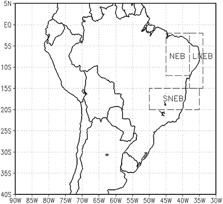
Figure 1. Areas of the Northeast of Brazil used in this study: Semiarid region in Northeastern Brazil (NEB), Easternern NNB (LNEB), Southern NNB (SNEB).

Data and Methodology

Observational Data

Monthly data from the Global Precipitation Climatology Project (GPCP, Adler et al., 2003) and the Climate Prediction Center Merged Analysis of Precipitation (CMAP, Xie and Arkin, 1997) were utilized as observed rainfall. These two data sets are plotted in grid points of 2.5 × 2.5° of latitude and longitude over the entire globe.

As observed SST dataset, it was used the Extended Reconstructed Sea Surface Temperature (ERSST) version 3b from 1970 to 1999, these data are 2 × 2° gridded monthly mean derived from International Comprehensive Ocean-Atmosphere Data Set (ICOADS) and use several statistical methods that allow reconstruction using scarce data (Smith et al., 2008).

Data from the Climate Models

The CMIP3-AR4 and CMIP5-AR5 data are monthly rainfall totals (Table 1). The runs of these models relate to the so-called C20 (the twentieth century) and to the climate change scenarios A2 and RCP8.5 of the models AR4 and AR5 (CMIP5, 2014), respectively. The C20 period chosen was from 1979–2000 because the network of observations of meteorological data over South America became denser during this period, in addition to the increasing availability of satellite data. The information on the volume of greenhouse gases in scenarios A2 and RCP8.5 can be found in detail on the site http://www-pcmdi.llnl.gov/.

TABLE 1

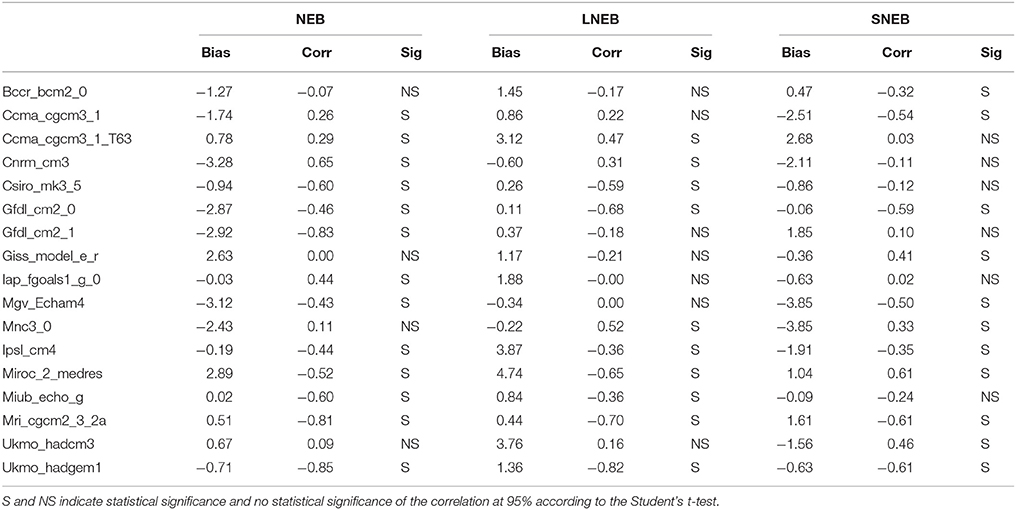
Table 1. Correlation and bias between the summer rainfall simulated by the CMIP3 models and the observations in CMAP.

Analysis Techniques

For the observed and simulated data (C20, A2, and RCP8.5), monthly and seasonal rainfall means (DJF and MAM) were calculated for the previously cited areas in Northeastern Brazil (Figure 1) for the periods 1970–2000 (experiment C20) and 2070–2100 (scenarios A2 and RCP8.5).

To compare the observed data and simulated data using the models in each region, the Pearson correlation coefficient, the correlation coefficient and the absolute error (bias) were used. The correlation and bias were determined between the rainfall simulated by the CMIP3 and CMIP5 models and the observations in CMAP. The bias indicates how much the simulated values are underestimated or overestimated in relation to the observed values.

Results and Discussion

Semiarid Region of the Northeast (NEB)

Figure 2 shows the monthly rainfall climatology (December–January) for the driest region of the Northeast during the period 1979–2000 according to the data observed from the CMAP and simulated by the models from the CMIP3-AR4. We can see that most models simulating the annual rainfall cycle of this region overestimate the rainfall in March. Among the 16 models analyzed, only four models (GDFL_CM2_1, Hadagem1, Miroc_2_medres, Giss_m_er) were not able to capture the annual rainfall cycle in this region.

FIGURE 2

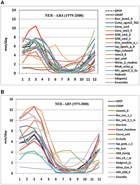
Figure 2. Annual rainfall cycle observed (GPCP and CMAP) for the NEB over the period 1979–2000 and simulated CMIP3-AR4 (A) CMIP5-AR4 (B) models.

Figure 2 also reveals that between the months of January and June, nearly half of the AR4 models overestimate the mean monthly rainfall, including during the wettest months in NEB (March and April). In the preseason period (November and December), on the other hand, the models generally underestimate the observed rainfall. This characteristic could be explained because the models are not able to capture the transient atmospheric systems acting in this region as upper cyclonic vortexes. The multi-model ensemble is more consistent with the annual climatology of the semiarid region of NNEB (gray line in Figure 2). During the drier period from July to September, the analyzed models also underestimate the rainfall.

For the CMIP5-AR5 models (Figure 2B), similar characteristics to those of the AR4 models are observed for the semiarid region of NNEB. Most models have a positive bias, overestimating the observed rainfall in the first 6 months and the rainy season of the region. Between July and October, the region's dry season, the models tend to produce lower values than those observed. Two out of the 14 models analyzed are not able to reproduce the annual cycle of the region, Giss_e3_r_ce and EC_Earth.

Eastern Region of the Northeast (LNEB)

In the eastern region of the Northeast, where the rainy season prevails from April to July, the models do not efficiently simulate the annual rainfall cycle as they do in the semi-arid region. Although some models simulate the annual rainfall cycle, most tend to significantly overestimate or underestimate the mean rainfall values (Figure 3). The models GFDL_CM2_1, GISS_model_ER and HADGEM1 did not simulate the annual rainfall cycle in this region.

FIGURE 3

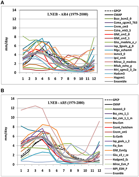
Figure 3. Annual rainfall cycle observed (GPCP and CMAP) for the LNEB over the period 1979–2000 and simulated CMIP3-AR4 (A) CMIP5-AR4 (B) models.

This region, which is a coastal area of NNEB, suffers great influences from meso and local scale atmospheric systems, and the models considered cannot adequately resolve the physical processes that occur on a smaller scale than their horizontal resolution. Therefore, they do not reproduce the rainfall in a satisfactory manner, bringing down the performance of these models in the simulation of the seasonal cycle.

The CMIP5-AR5 models also performed worse in the simulation of the annual rainfall cycle over the LNEB sector, just as could be seen in most CMIP3-AR4 models (Figures 4A,B). The models overestimate rainfall during the wettest months when compared to observations, while they underestimate it during the drier period. As in the previous analyses, there are some models that are unable to capture the annual rainfall cycle in the LNEB (EC-Earth and Giss_er-Ce). The spatial resolution of the Climate Global Models has been increased from CMIP3 to CMIP5 in addition to improvements in physical parameterization regarding cloud and radiation processes (Dolinar et al., 2015); however better representation of coastal areas is still lacking due to the underlying grid spacing of the models (Nicholls et al., 2007; Flato et al., 2013), which leads to growing uncertainty about the impacts of climate change regarding precipitation in these regions.

FIGURE 4

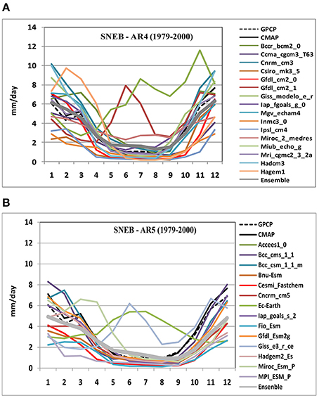
Figure 4. Annual rainfall cycle observed (GPCP and CMAP) for the SNEB over the period 1979–2000 and simulated CMIP3-AR4 (A) CMIP5-AR4 (B) models.

Southern of the Northeast (SNEB)

Figure 4 shows how the CMIP3-AR4 and CMIP5-AR5 models simulate the annual rainfall cycle (1979–2000) for the southern region of NNEB. Most models are able to simulate the annual rainfall cycle in this region (beginning in October and ending March–April), with the exception of models GFDL_CM2_1, GISS_model_E_Rr and HADGEM1. When the average of the CMIP3 models (gray line) is considered, there is good consistency between the observations and the simulations.

The CMIP5-AR5 models also capture the annual rainfall cycle over SNEB, except for the models EC-EARTH and GISS_E3_R_CE. The models MPI_ESM_P and FIO_ESM sharply underestimated the rainfall in this region, despite representing the annual cycle (Figure 4).

Analysis of the Seasonal Variability in Average over NEB, LNEB, and SNEB: Correlations and Absolute Error

The correlation and bias between the summer rainfall simulated by the CMIP3 models and the observations in CMAP for the 1979–2000 periods are analyzed. Tables 1–4 show the results obtained for the summer and autumn in the CMIP3 and CMIP5 models. As can be seen in Table 1, the CMIP3 models tend to underestimate the rainfall in the Semiarid and SNEB regions, and to overestimate it in LNEB. The CNRM_CM3 model obtained the highest correlation coefficients for NEB in summer (0.65), followed by the MNC3_0 model for the LNEB (0.52), and by the Miroc_2_MEDRES for the SNEB with a coefficient about 0.6.

In the autumn, the CMIP3 models tend to underestimate the rainfall in the semiarid regions of NNEB and to overestimate it in LNEB and SNEB (Table 2). The highest correlations were found for the model Ipsl_cm4, with a coefficient of 0.78 for NEB and SNEB, and for the model Miub_echo_g with correlation of 0.74.

TABLE 2

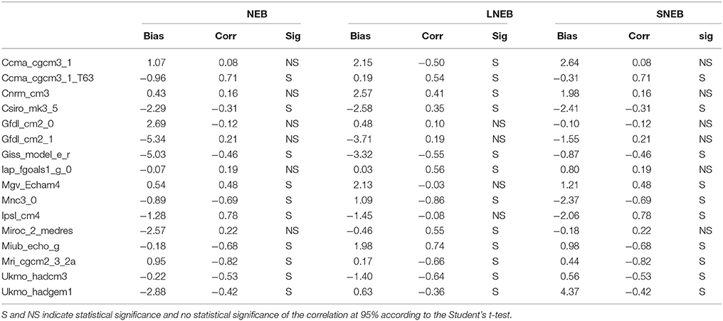
Table 2. Correlation and bias between the autumn rainfall simulated by the CMIP3 models and observations in CMAP.

For the CMIP5 models, the results are shown in Tables 3, 4. The CMIP5 models tend to overestimate the summer rainfall in the semiarid region of NNEB, and to underestimate it for LNEB and SNEB. The correlations were generally lower than those of the CMIP3 models. The models with the highest correlation coefficients were as follows: Ccma_cgcm3_1._T63 and Mri_cgcm2_3_2a with 0.39 for NEB, Miroc_2_med_res with 0.36 for the LNEB, and Mgv_Echam4 with 0.68 for the SNEB.

TABLE 3

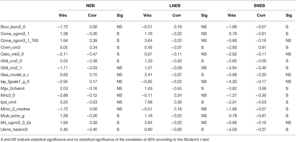
Table 3. Correlation and bias between the autumn rainfall simulated by the CMIP5 models and observations in CMAP.

TABLE 4

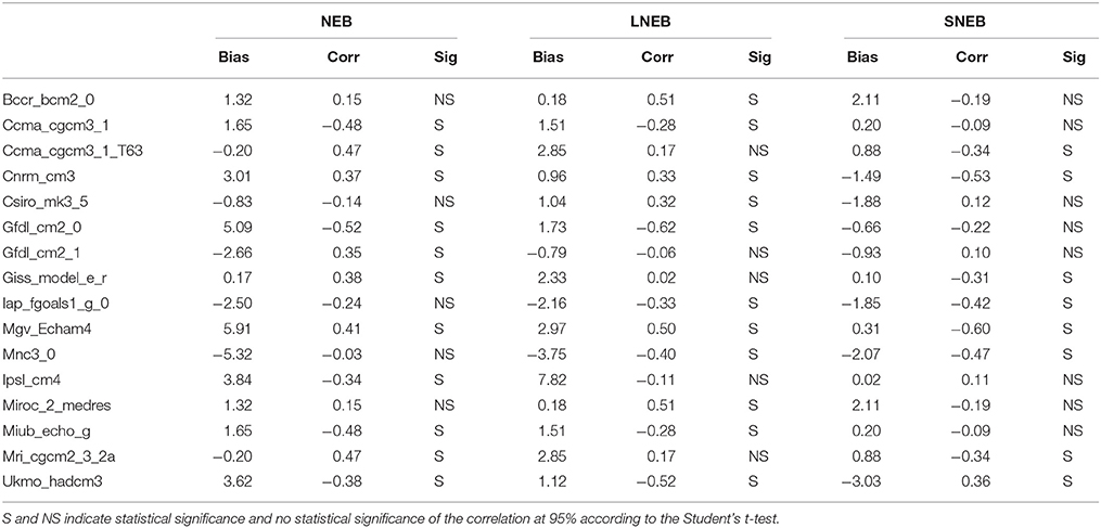
Table 4. Correlation and bias between the autumn rainfall simulated by the CMIP5 models and observations in CMAP.

In autumn (Table 4), the correlation characteristics were similar to those observed during the summer, but regarding bias, there was a predominance of rainfall overestimation in the simulations of the models.

Correlation maps of seasonal precipitation between models (CMIP3 and CMIP5) and observation during period 1979–2000 for DJF are presented in the Figures 5, 6, they showed few spots with statistical significance. These figures show the mean absolute error in addition to the correlation. In fact, during austral summer, the interannual precipitation variability is barely captured by the models, especially over Northeastern Brazil. In general, there are no noticeable improvements from CMIP3 to CMIP5 during this period. Even though mostly models present large mean absolute errors over the Tropical Atlantic and Northeastern South America, three models from CMIP3 (Gfdl_cm2_0, Ipsl_cm4, and Iap_goals_1_0_g) show correlations statistically significant over NEB (Figures 5E,H,K). The errors on Northeastern Brazil from these models are quite small in comparison those from the other models. It is worth mentioning that just BNU_ESM (Figure 6D) provides good results over Northeast Brazil and Tropical Atlantic, indicating that this model is able to represent the interannual variability during austral summer, depicted in terms of skill and mean absolute error.

FIGURE 5

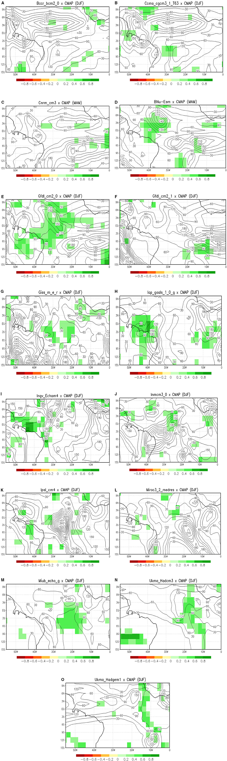
Figure 5. Correlation (shaded) and absolute error (contour in mm) to summer (DJF) between observation (CMAP) and simulation from CMIP3-AR4 models for period 1979–2000. The models considered are (A) Bccr_bcm2_0, (B) Ccma_cgcm3_1_T63, (C) Cnrm_cm3, (D) BNu_Esm, (E) Gfdl_cm2_0, (F) Gfdl_cm2_1, (G) Giss_m_e_r, (H) Iap_goals_1_0, (I) Ingv_ECHAM4, (J) Inmcm3_0, (K) Ipsl_cm4, (L) Miroc3_2_medres, (M) Miub_echo_g, (N) Ukmo_Hadcm3, and (O) Ukmo_Hadgem1. Green areas indicate statistical significance of the correlation at 95% according to the Student's t-test.

FIGURE 6

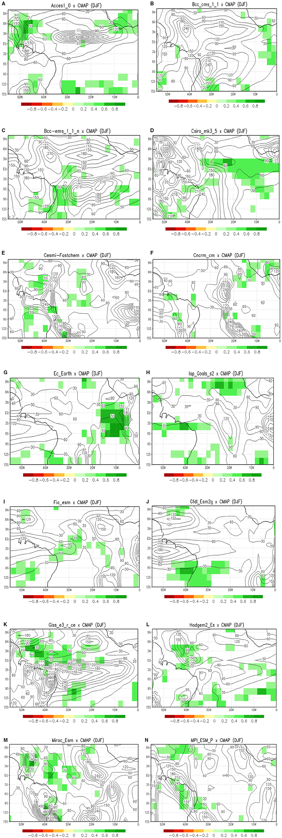
Figure 6. Correlation (shaded) and absolute error (contour in mm/day) to summer (DJF) between observation (CMAP) and simulation from the CMIP5-AR5 models for period 1979–2000. Models considered are: (A) Access1_0, (B) Bcc_cms_1_1, (C) Bcc_ems_1_1, (D) Csiro_mk3_5, (E) Cesmi-Fastchem, (F) Cncrm_cm, (G) Ec_Earth, (H) Iap_Goals, (I) Fio_esm, (J) Gfdl_Esm2g, (K) Giss_e3_r_ce, (L) Hadgem2_ES, (M) Miroc_Esm, and (N) MPI_ESM_P. Green areas indicate statistical significance of the correlation at 95% according to the Student's t-test.

For the period of austral autumn (MAM), the results are similar to DJF. Primarily, the models have difficulty capturing the precipitation variability over Northeastern Brazil and the Tropical Atlantic (Figures 7, 8). High mean absolute errors in South America are observed in the CMIP3 simulations. Nevertheless a couple of models, such as Iap_goas_1_0_g and Gfdl_cm2_0, have shown satisfactory results with significant correlations over northern Northeastern Brazil and over the Tropical Atlantic, respectively (Figures 7E,H). These models are able to minimally solve the convection and the displacement of the Intertropical Convergence Zone on the Northeastern coast. The CMIP5 models, Gfdl_esm2g and Bnu_esm, (Figures 8D,J) are barely able to reproduce the temporal variance of the observed rainfall near the NEB coast, with a correlation between 0.5 and 0.7, although over the continent, high mean absolute errors greater than 100 mm are assigned. In general, the models continue to show poor performance in capturing the accumulated precipitation over the period analyzed (1979–2000); large errors along with a few points with significant correlation are found in NNEB.

FIGURE 7

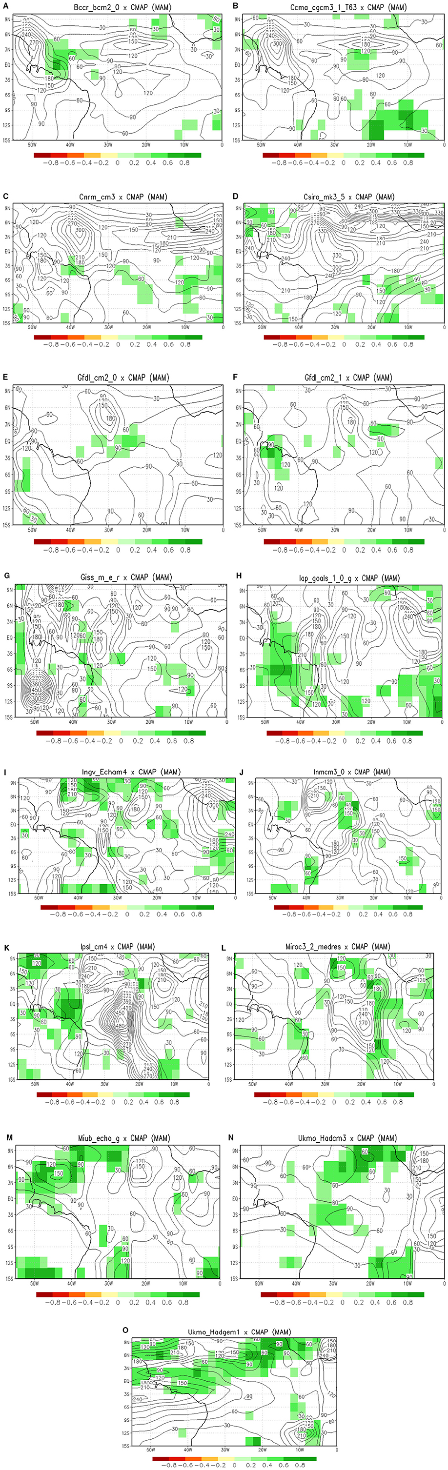
Figure 7. Correlation (shaded) and absolute error (contour in mm/day) to austral autumn (MAM) between observation (CMAP) and simulations from the CMIP3-AR4 models for period 1979–2000. The models considered are: (A) Bccr_ccm2_0, (B) Ccma_cgcm3_1_T63, (C) Cnrm_cm3, (D) Csiro_mk3_5, (E) Gfdl_cm2_0, (F) Gfdl_cm2_1, (G) Giss_m_e_r, (H) Iap_goals_1_0_g, (I) Ingv_Echam4, (J) Inmcm3_0, (K) Ipsl_cm4, (L) Miroc3_2_medres, (M) Miub_echo_g, (N) Ukmo_hadcm3, and (O) Ukmo_Hadgem1. Green areas indicate statistical significance of the correlation at 95% according to the Student's t-test.

FIGURE 8

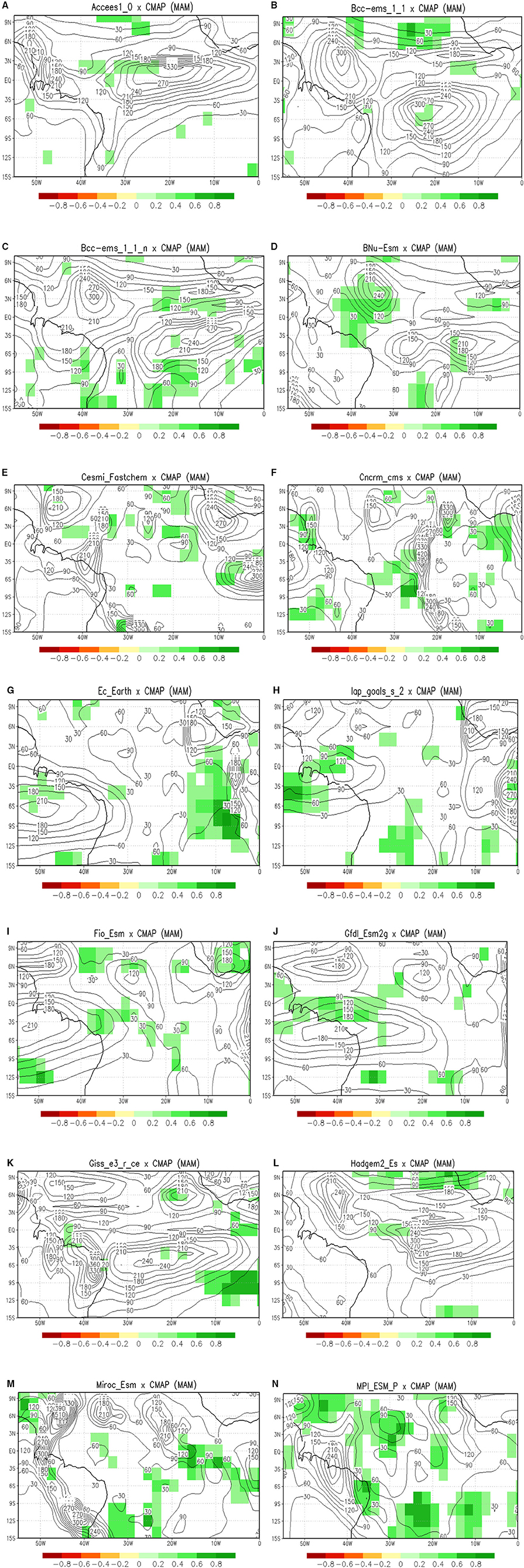
Figure 8. Correlation (shaded) and absolute error (contour in mm/day) to austral autumn (MAM) between observation (CMAP) and simulation from the CMIP5-AR5 models for period 1979–2000. The models considered are: (A) Access1_0, (B) Bcc_ems_1_1, (C) Bcc_ems_1_1_n, (D) BNu-Esm, (E) Cesmi_Fastchem, (F) Cncrm_cms, (G) Ec_Earth, (H) Iap_goals_s_2, (I) Fio_Esm, (J) Gfdl_Esm2g, (K) Giss_e3_r_ce, (L) Hadgem2_Es, (M) Miroc_Esm, and (N) MPI_ESM_P. Green areas indicate statistical significance of the correlation at 95% according to the Student's t-test.

The interannual variability of precipitation in the Northeast is associated with changes in sea surface temperature (SST) in the Tropical Atlantic (Moura and Shukla, 1981; Nobre and Shukla, 1996). Variations in zonal and meridional atmospheric circulation are influenced by ocean-atmosphere interaction in the Atlantic basin in response to the anomalous SST patterns. Therefore, a way to explain the lack of representation of the interannual variability of rainfall from the CMIP3 and CMIP5 models is to investigate how these coupled models represent the two leading modes of variability in these regions (Servain et al., 2003). In this regard, the calculation of empirical orthogonal functions (EOF) was performed to isolate the principal modes of variability during DJF and MAM from 1970 to 2000.

The results show that the models are deficient in representing the SST variability modes in the tropical Atlantic. Low explained variance and changes in the order of the modes are issues faced by the models. Here, we just show the analysis of the loading scores (PC: Principal Components), i.e., the time series indicating how the spatial patterns vary over time. The representation of spatial modes will be discussed in another paper in preparation.

Table 5 shows the correlation between the loading scores from two leading EOFs (PC1 and PC2) observed and simulated by the CMIP3 models for DJF and MAM. Values with low correlation and not statistically significant are shown in the results; a few models achieve significant correlations. Two of them had significant values for the two leading PCs, ipsl_cm3 for DJF and Cnrm_esm for MAM, despite the low values; they generate a lack of representation of the rainfall variability over NNEB and the tropical Atlantic.

TABLE 5

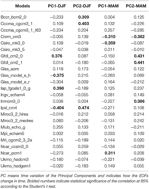
Table 5. Correlation between observational and simulated (CMIP3 models) loading scores (PC1 and PC2) for DJF and MAM SST anomalies.

Even increasing the resolution of the CMIP5 models and improvements in the physics of ocean and atmospheric models, they continue to present problems in representing the patterns of SST variability in the tropical Atlantic (Table 6). The models fail to follow the temporal variability of observed patterns, even in examples such as HADGEM2_AO, which indicates a correlation of about 0.6 in PC2 and presents a null value for PC1.

TABLE 6

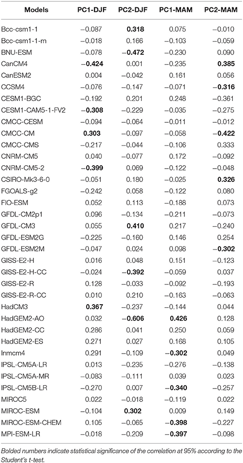
Table 6. Same as Table 5, except for CMIP5 models.

Climate Projections (2040–2070)

In this section, the projections of the CMIP3 and CMIP5 models for rainfall in the period of 2040–2070 are analyzed. The summer and autumn months are considered in this analysis because most of the rainfall over NEB occurs in these seasons. This periods (2040–2070) includes a large portion of the so-called midslice period of the protocol of analyses proposed for future climate projections by the IPCC (Taylor et al., 2007). In this article, we do not discussion the possible causes for why these CMIP3 and CMIP5 models do not represent these thermal modes in the tropical Atlantic Basin.

Semiarid Region of the Northeast (NEB)

Figures 9–14 show the rainfall anomalies (mm/day) of the CMIP3 and CMIP5 models for the period 2040–2070 in relation to the historic reference period of 1971–2000 for the summer (November to January) and autumn (February to April).

FIGURE 9

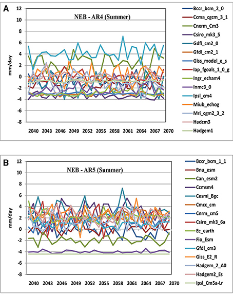
Figure 9. Summer rainfall anomalies projected for semiarid region of NNB from CMIP3-AR4 (A) and CMIP5-AR4 (B) models over the period 2040–2070.

FIGURE 10

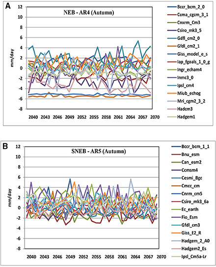
Figure 10. As Figure 9 except for autumn.

FIGURE 11

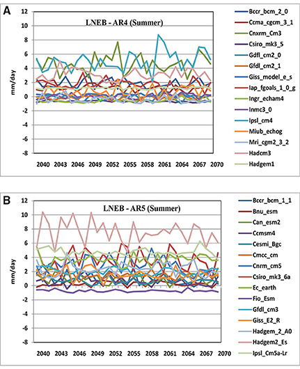
Figure 11. Summer rainfall anomalies projected for eastern NNB from CMIP3-AR4 (A) and CMIP5-AR4 (B) models over the period 2040-2070.

FIGURE 12

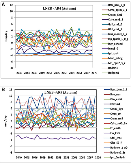
Figure 12. As Figure 11 except for autumn.

FIGURE 13

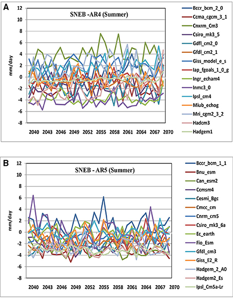
Figure 13. Summer rainfall anomalies projected for southern NNB from CMIP3-AR4 (A) and CMIP5-AR4 (B) models over the period 2040-2070.

FIGURE 14

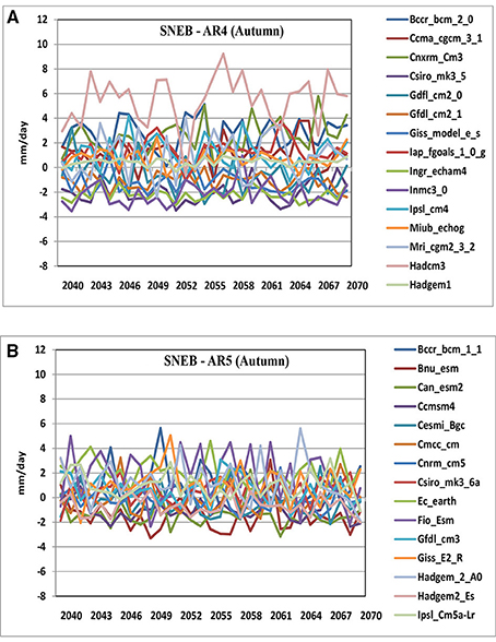
Figure 14. As Figure 13 except for autumn.

A divergence in the projections of the rainfall signal can be seen when the two phases of the CMIP are compared. While the CMIP3 projections for summer and autumn (Figures 9A, 10A, 11A, 12A, 13A, 14A) reveal a predominance of rainfall below the mean, the projections of the CMIP5 models show a rainfall trend that is above the mean (Figures 9B, 10B, 11B, 12B, 13B, 14B) to around the mean (1979–2000) in most of the models. In the results of Christensen et al. (2013), the analyses done with the CMIP5 models for Northeastern Brazil also demonstrate this characteristic of above average rainfall in the projections for the twenty-first century. However, more CMIP5 than CMIP3 models were analyzed.

Eastern Region of the Northeast (LNEB)

The projected rainfall for the summer/autumn of 2040–2070 in the eastern part of NNEB is similar in the CMIP3 and CMIP5 models. Figures 11A,B, 12A,B show these characteristics, with a predominance of rainfall anomalies around or above the mean throughout the period of 2040–2070 in most of the models analyzed. This characteristic, however, is more evident in the CMIP5 models (Figure 12B).

Southern Region of the Northeast (SNEB)

The rainfall projections for the southern of the Northeast for the summer in 2040–2070 do not show a clear signal of the precipitation anomalies in this region in the CMIP3 models (Figure 13A). In the CMIP5 models, however, there is predominance of rainfall anomalies around and above the mean (Figure 13B).

In the CMIP3 models for the autumn period of 2040–2070 (Figure 14A), there is a greater number of models with rainfall projections around to above the mean. The CMIP5 models revealed a large interannual variability, and no trend could be observed for the rainfall anomaly signal in this region during the period considered (Figure 14B).

Conclusions and Recommendations

According to the analysis, the following conclusions can be drawn from the study. The CMIP3 and CMIP5 models proved to have a good sensitivity to reproduce the annual rainfall cycle in the three areas of NEB chosen for this analysis: the semiarid, eastern and southern regions of the NNEB.

The analysis of the metrics to investigate how the CMIP3 and CMIP5 models simulate the monthly variations in the summer and autumn seasons in these regions of the NNEB revealed that some models are able to simulate this monthly variability with better performance. The ability of the Climate Global Models seems to be an issue due their spatial resolution to depict seasonal precipitation on coastal areas. On the other hand, Regional Climate Modeling has emerged as alternative to succeed in dealing with meso-local physical process, topography, heterogeneity of land-use and vegetation cover, hence producing robust aspects about regional climate change (Giorgi and Gutowski, 2015). Statistical downscaling also could be a tool to overcome this issue, Silva and Mendes (2015) showed advances doing refinement of representation of daily precipitation in NNEB from CMIP5-AR5 models.

Modes of SST variability in tropical Atlantic Ocean modulate the interannual rainfall anomalies over NEB (Servain, 1991); in our EOF analysis of the Tropical Atlantic SST the CMIP3-AR4 and CMIP5-AR5 models do not properly capture the temporal variation of the PCs. In general, the most models face problems to solve atmospheric-ocean interaction and internal variability what may explain the misrepresentation of SST anomalies patterns and, consequently, the lack of seasonal precipitation skill over NNEB.

When the summer and autumn rainfall projections for the period 2040–2070 for the driest region of the NEB were considered, there was no convergence between the CMIP3 and CMIP5 models. In general, the CMIP3 (CMIP5) models project rainfall near (above) the reference mean. In the summer and autumn of the eastern sector of NEB, both the CMIP3 and CMIP5 models projected above the mean rainfall for the 2040–2070 period. For the SNEB sector, the projections indicate rainfall oscillating around the mean in the summer according to the CMIP3 models and below the mean in the CMIP5 models. In the autumn, most CMIP3 models projected rainfall around the mean, while the CMIP5 models revealed a predominance of rainfall around or above the mean.

For future studies, a more detailed analysis is suggested of the average monthly thermal cycle of the eastern and southern regions of the NNEB, in addition to the extension of these analyses to the north of the Amazon (area of native tropical forest), the southeastern Amazon (area with great impact of the use and occupation of the soil), southeast of South America (area that encompasses a region of high urban concentration and energy production). Additionally, the ability of the CMIP3 and CMIP5 models to simulate and project the gradients of Sea Surface Temperature (SST) in the Atlantic Ocean, which has a strong influence on the tropical climate of the Americas and Africa, should also be studied.

Author Contributions

JA, Article idea of the author and responsible for the analyzes under discussion. RC, Article idea of the author and responsible for the analyzes under discussion. ES, Collaborator in the analysis of results and discussions presented. AC, Collaborator in the analysis of results and discussions presented. AB, Collaborator in the analysis of results and discussions presented. SS, Collaborator in the analysis of results and discussions presented. FV, Collaborator in the analysis of results and discussions presented. AD Collaborator in the analysis of results and discussions presented. JS Collaborate in the analysis of results and discussions presented.

Conflict of Interest Statement

The authors declare that the research was conducted in the absence of any commercial or financial relationships that could be construed as a potential conflict of interest.

Acknowledgments

JA thanks the Coordenação de Aperfeiçoamento de Pessoal de Nível Superior (CAPES), by Postdoctoral Junior (Project No. 23038.007455 / 2011-95 PNPD CAPES-UFRN, as part of the Institutional Project Postdoctoral Program 2011, coordinated by RC. JS is grateful to CNPq for the grant associated with Project Mudanças Climáticas no Atlântico Tropical (MUSCAT), Process 400544/2013-0. FUNCEME (Project BTT FUNCEME/FUNCAP, Edital 09/2015) is acknowledged for its support while JS visited Fortaleza, CE, Brazil. The authors would like to thank two reviewers for providing constrictive criticisms that improved the quality of the paper.

References

Adler, R. F., Huffman, G. J., Chang, A., Ferraro, R., Xie, P.-P., Janowiak, J., et al. (2003). The Version 2 Global Precipitation Climatology Project (GPCP) monthly precipitation analysis (1979 - present). J. Hydrometeor. 4, 1147–1167. doi: 10.1175/1525-7541(2003)004<1147:TVGPCP>2.0.CO;2

CrossRef Full Text | Google Scholar

Bernstein, L., Bosch, P., Canziani, O., Chen, Z., Christ, R., Davdson, O., et al. (2007). Climate Change. Synthesis Report. IPCC, Londres.

Christensen, J. H., Krishna Kumar, K., Aldrian, E., An, S.-I., Cavalcanti, I. F. A., Zhou, M., et al. (2013). “Climate phenomena and their relevance for future regional climate change,” in Climate Change (2013). The Physical Science Basis. Contribution of Working Group I to the Fifth Assessment Report of the Intergovernmental Panel on Climate Change, eds T. F. Stocker, D. Qin, G.-K. Plattner, M. Tignor, S. K. Allen, J. Boschung et al. (Cambridge, UK; New York, NY: Cambridge University Press), 204.

CMIP5. (2014). Coupled Model Intercomparison Project. Available online at: http://cmip-pcmdi.llnl.gov/cmip5/

Collins, J. M., Chaves, R. R., and da Silva Marques, V. (2009). Temperature variability over South America. J. Clim. 22, 5854–5868. doi: 10.1175/2009JCLI2551.1

CrossRef Full Text | Google Scholar

Collins, W. D., Bitz, C. M., Blackmon, M. L., Bonan. G. B., Bretherton, C. S., Carton, J. A., et al. (2006). The Community Climate System Model version 3 (CCSM3). J. Clim. 19, 2122–2143. doi: 10.1175/JCLI3761.1

CrossRef Full Text | Google Scholar

Dolinar, E, K., Dong, X., Xi, B., Jiang, J., and Su, H. (2015). Evaluation of CMIP5 simulated clouds and TOA radiation budgets using NASA satellite observations. Clim. Dyn. 44, 2229–2247. doi: 10.1007/s00382-014-2158-9

CrossRef Full Text | Google Scholar

Endo, N., Ailikun, B., and Yasunary, T. (2005). Trends in precipitation amounts and the number of rainy days and heavy rain events during summer in China from 1961 to 2000. J. Meteorol. Soc. Jpn. 83, 621–631. doi: 10.2151/jmsj.83.621

CrossRef Full Text | Google Scholar

Flato, G., Marotzke, J., Abiodun, B., Braconnot, P., Chou, S. C., Rummukainen, W., et al. (2013). “Evaluation of climate models,” in Climate Change 2013: The Physical Science Basis. Contribution of Working Group I to the Fifth Assessment Report of the Intergovernmental Panel on Climate Change, eds T. F. Stocker, D. Qin, G. -K. Plattner, M. Tignor, S. K. Allen, J. Boschung et al. (Cambridge, UK; New York, NY: Cambridge University Press), 741–882.

Garreaud, R. D., Vuille, M., Compagnucci, R., and Marengo, J. (2009). Present day South American climate. Palaeogeogr. Palaeoclimatol. Palaeoecol. 281, 180–195. doi: 10.1016/j.palaeo.2007.10.032

CrossRef Full Text | Google Scholar

Gemmer, M., Becker, S., and Jiang, T. (2004). Observed monthly precipitation trends in China 1951-2002. Theor. Appl. Climatol. 77, 39–45. doi: 10.1007/s00704-003-0018-3

CrossRef Full Text | Google Scholar

Giorgi, F., and Gutowski, W. J. Jr. (2015). Regional dynamical downscaling and the CORDEX initiative. Annu. Rev. Environ. Resour. 40, 467–490. doi: 10.1146/annurev-environ-102014-021217

CrossRef Full Text | Google Scholar

Haylock, M. R., Peterson, T. C., Alves, L. M., Ambrizzi, T., Anunciação, M. T., Baez, J., et al. (2006). Trends in total and extreme South American rainfall in 1960-2000 and links with sea surface temperature. J. Clim. 19, 1490–1512. doi: 10.1175/JCLI3695.1

CrossRef Full Text | Google Scholar

IPCC (2007). “Summary for policymakers. Climate change,” in The Physical Science Basis. Contribution of Working Group I to the Fourth Assessment Report of the Intergovernmental Panel on Climate Change, eds S. Solomon, D. Qin, M. Manning, Z. Chen, M. Marquis, K. B. Averyt et al. (Cambridge, UK; New York, NY: Cambridge University Press), 18.

IPCC (2013). “Climate change. The physical science basis,” in Contribution of Working Group I to the Fifth Assessment Report of the Intergovernmental Panel on Climate Change, eds T. F. Stocker, D. Qin, G.-K. Plattner, M. Tignor, S.K. Allen, J. Boschung et al. (Cambridge, UK; New York, NY: Cambridge University Press), 1535.

IPCC (2014). “Summary for policymakers. Climate change,” in Impacts, Adaptation, and Vulnerability. Part A: Global and Sectoral Aspects. Contribution of Working Group II to the Fifth Assessment Report of the Intergovernmental Panel on Climate Change, eds C. B. Field, V. R. Barros, D. J. Dokken, K. J. Mach, M. D. Mastrandrea, T. E. Bilir et al. (Cambridge, UK; New York, NY: Cambridge University Press), 1–32.

Kalnay, E., Kanamitsu, M., Kistler, R., Collins, W., Deaven, D., Joseph, L., et al. (1996). The NCEP/NCAR 40-year reanalysis project. Bull. Am. Meteorol. Soc. 77, 437–471.

Google Scholar

Marengo, J. A. (May, 2009). Future change of climate in South America in the late 21st century: the CREAS Project. AGU AS Newsletter. P. 5.

Marengo, J. A., Ambrizzi, T., Da Rocha, R. P., Alves, L. M., Cuadra, S. V., Valverde, M. C., et al. (2009). Future change of climate in South America in the late twenty-first century: intercomparison of scenarios from three regional climate models. Clim. Dynam. 35, 1073–1097. doi: 10.1007/s00382-009-0721-6

CrossRef Full Text | Google Scholar

Marengo, J. A., and Valverde, M. C. (2007). Caracterização do clima no Século XX e Cenário de Mudanças de clima para o Brasil no Século XXI usando os modelos do IPCC AR4. Revista Multiciência (Portuguese) 8, 5–28.

Google Scholar

Meinshausen, M., Smith, S. J., Calvin, K., Daniel, J. S., Kainuma, M. L. T., Lamarque, J.-F., et al. (2011). The RCP greenhouse gas concentrations and their extensions from 1765 to 2300. Clim. Change 109, 213–241. doi: 10.1007/s10584-011-0156-z

CrossRef Full Text | Google Scholar

Moura, A. D., and Shukla, J. (1981). On the dynamics of droughts in Northeast Brazil: observations, theory and numerical experiments with a general circulation model. J. Atmospherical Sci. 38, 2653–2675. doi: 10.1175/1520-0469(1981)038<2653:OTDODI>2.0.CO;2

CrossRef Full Text | Google Scholar

Nicholls, R. J., Wong, P. P., Burkett, V. R., Codignotto, J. O., Hay, J. E., Woodroffe, R. F., et al. (2007). “Coastal systems and low-lying areas,” in Climate Change 2007: Impacts, Adaptation and Vulnerability. Contribution of Working Group II to the Fourth Assessment Report of the Intergovernmental Panel on Climate Change, eds M. L. Parry, O. F. Canziani, J. P. Palutikof, P. J. van der Linden, and C. E. Hanson (Cambridge, UK: Cambridge University Press), 315–356.

PubMed Abstract

Nobre, P., and Shukla, J. (1996). Variations of sea surface temperature, wind stress, and rainfall over the tropical Atlantic and South America. J. Clim. 10, 2464–2479. doi: 10.1175/1520-0442(1996)009<2464:VOSSTW>2.0.CO;2

CrossRef Full Text | Google Scholar

Qin, D. H., Ding, Y. H., Su, J. L., and Wang, S. M. (2005). Climate and environment changes in China. China Science Press, 562p.

PubMed Abstract

Servain, J. (1991). Simple climatic indices for the tropical Atlantic Ocean and some applications. J. Geophys. Res. 96, 15137–15146. doi: 10.1029/91JC01046

CrossRef Full Text | Google Scholar

Servain, J., Clauzet, G., and Wainer, I. C. (2003). Modes of tropical Atlantic climate variability observed by PIRATA. Geophys. Res. Lett. 30:8003. doi: 10.1029/2002GL015124

CrossRef Full Text | Google Scholar

Silva, G. A., and Mendes, D. (2015). Refinement of the daily precipitation simulated by the CMIP5 models over the north of the Northeast of Brazil. Front. Environ. Sci. 3:29. doi: 10.3389/fenvs.2015.00029

CrossRef Full Text | Google Scholar

Smith, T. M., Reynolds, R. W., Peterson, T. C., and Lawrimore, J. (2008). Improvements to NOAA's historical merged land-ocean surface temperature analysis (1880-2006). J. Clim. 21, 2283–2296. doi: 10.1175/2007JCLI2100.1

CrossRef Full Text | Google Scholar

Taylor, K. E., Crucifix, M., Braconnot, P., Hewwit, C. D., Doutriaux, C., Broccoli, A. J., et al. (2007). Estimating shortwave radiative forcing and response in climate models. J. Clim. 29, 2530–2543. doi: 10.1175/JCLI4143.1

CrossRef Full Text | Google Scholar

Taylor, K. E., Stouffer, R. J., and Meehl, G. A. (2012). An overview of CMIP5 and the experiment design. Bull. Am. Meteorol. Soc. 93, 485–498. doi: 10.1175/BAMS-D-11-00094.1

CrossRef Full Text | Google Scholar

Tolen, J., Kodra, E. A., and Ganguly, A. R. (2011). “Comparative evaluation of the IPCC AR5 CMIP5 versus the AR4 CMIP3 model ensembles for regional precipitation and their extremes over South America,” in AGU Fall Meeting Abstracts, Vol. 1 (São Francisco, CA), 1047.

Vera, C., Silvestre, G., Liebman, B., and Gonzáles, P. (2006). Climate change scenarios for seasonal precipitation in South America from IPCC-AR4 models. Geophys. Res. Lett. 33, L13707. doi: 10.1029/2006GL025759

CrossRef Full Text | Google Scholar

Vicent, L. A., Peterson, T. C., Barros, V. R., Mariano, M. B., Rusticucci, M., Carrasco, G., et al. (2005). Observed trends in indices of daily temperature extremes in South America 1960–2000. J. Clim. 18, 5011–5023. doi: 10.1175/JCLI3589.1

CrossRef Full Text | Google Scholar

Wilby, R. (2008). A review of climate change scenarios for Northeast Brazil. Tear fund is a Christian relief and development agency building a global network of local churches to help eradicate poverty. Londres. 23.

Xie, P., and Arkin, P. A. (1997). Global Precipitation: A 17-year monthly analysis based on gauge observations, satellite estimates, and numerical model outputs. Bull. Am. Meteorol. Soc. 78, 2539–2558.

Google Scholar