Off Limits: Sulfate below the Sulfate-Methane Transition

Introduction

In recent years, it has become evident that the classical view of sedimentary sulfur cycling is incomplete, and may in important aspects be incorrect. There is growing evidence that sulfur cycling occurs outside of the main sulfate reduction zone. In these environments, sulfur compounds are continuously reduced and re-oxidized, with the overall inventory of the sulfur constituents remaining constant. This sulfur cycle so far has eluded direct observation, and has been coined cryptic sulfur cycling.

For example, cryptic sulfur cycling is inferred to occur in the oxygen minimum zone off Peru where sulfide that is produced by microbial sulfate reduction in the oxygen-free core of oxygen minimum zones is converted back to sulfate, presumably tied to reductive nitrogen cycling (Canfield et al., 2010b; Teske, 2010; Johnston et al., 2014). Another example for the potential of cryptic sulfur cycling comes from a sub-glacial lake in Antarctica (Mikucki et al., 2009), where sulfate-sulfur is apparently reduced and re-oxidized back to sulfate via coupling to reductive iron cycling. The finding of sulfate reducing microorganisms in in subsurface methanic sediments from Aarhus Bay (Baltic Sea) and Black Sea sediments (Leloup et al., 2007, 2009) that were traditionally considered to be sulfate-free and devoid of active sulfate reduction, and the presence of low, but detectable sulfate in subsurface methanic sediments from Aarhus Bay (Holmkvist et al., 2011) implies that cryptic sulfur cycling is an ongoing process throughout the anoxic sediment column.

The potential existence of a cryptic sulfur cycle beneath the main sulfate zone in marine sediments is particularly interesting. It challenges or at least transforms the paradigm that there is a sequential cascade of electron accepting processes in the environment across redox gradients, with the energetically most favorable electron acceptor being consumed first and the least attractive process being carried out last (i.e., in marine organic-rich sediments: oxygen respiration, nitrate, manganese, iron, and, sulfate reduction, methanogenesis). In the methanic zone, sulfate is assumed to have been completely consumed because microbial sulfate reduction occurs even at very low sulfate concentrations (Tarpgaard et al., 2011) and because sulfate reduction can be coupled to the anaerobic oxidation of methane. The finding of sulfate, and the persistence of sulfate reducing micororganisms in the methanic zone thus indicate that there is hidden, “cryptic” sulfate production in these sediments. Elucidating the mechanisms behind such sulfate production has the potential to gain new insights into the links between the biogeochemical cycles of different elements. For example, sulfide concentrations typically decrease below the sulfate-methane transition (SMT), presumably due to concomitant formation of pyrite (FeS₂), a process that necessitates sulfur oxidation. This demonstrates that in methanic sediments there is at least a potential for the availability of oxidants, such as reactive ferric iron, as invoked by Holmkvist et al. (2011) to explain the elevated concentrations of sulfate present below the SMT. Quantification of such a cryptic iron-sulfur cycle would shed light on how reactive such iron phases are, and to what extent microbial activity impacts the reactivity of the iron phases. An alternative avenue for the production of sulfate in methanic sediments could be the disproportionation of sulfur species with an intermediate oxidation state, which raises that question if, and under what circumstances, microbial sulfate reduction does not have sulfide as final metabolic product. This may be the case for in sulfate reduction coupled to the anaerobic oxidation of methane (Milucka et al., 2012) where zero-valent sulfur has been found to be an intermediate, but may even apply to classical microbial sulfate reduction (Bishop et al., 2013). As such, the exploration of cryptic sulfur cycling provides insight into how microbial processes under energy limitation work, and if/how specialized microorganisms share the already small amount of available energy to carry out different biochemical reactions.

The aim of this study was to investigate if sulfate production occurs below of the SMT in a setting that is typical for anaerobic marine sediments. This goal is pursued via the study of the sulfate concentration and the sulfate-sulfur and -oxygen isotope composition for two sediment cores retrieved from Aarhus Bay, Denmark.

Methods

Sediment and Pore Water Sampling

Two sediment cores, one in May and one in October 2013 were taken at Station M1 in Aarhus Bay (56°07.0580′N and 10°20.8650′E, Figure 1) during sampling campaigns aboard the RV Tyra. Previous studies have identified elevated sulfate concentrations below the SMT at this station (Holmkvist et al., 2011). Sediment cores were taken with a gravity corer which was constructed with a steel barrel with a 12 cm diameter PVC core liner. A 220-cm long core was collected in May 2013 and a 320-cm long core in October 2013, hereafter referred to as the Spring and Fall cores. Immediately after coring the ship returned to harbor and the cores were transported to cold rooms at Aarhus University where they were stored and processed at ~4°C.

FIGURE 1

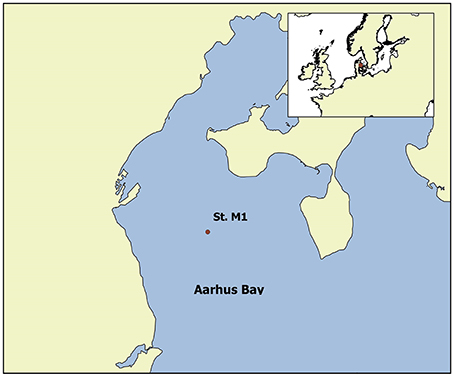
Figure 1. Map of study site and location of Station M1 in Aarhus Bay, Denmark.

In the Spring Campaign, all pore water samples were extracted using a Geotek^® pore water squeezer and a manual hydraulic press. Whole round core sections, 10 cm in length were cut, starting from the deepest part of the sediment core and proceeding step-wise to the shallowest portion. All sub-SMT pore water samples were collected and processed within 24 h of core retrieval (core-on-deck) and the remainder of pore water samples processed within the subsequent 27 h. Sediment sections were extruded from the liner and 1–2 cm of sediment were removed from the top, bottom, and sides of the core to remove any potential surface contamination or oxidation products. After this, the remaining sediment was loaded into the pore water squeezer. During loading, the pore water squeezer was continuously back-flushed with nitrogen gas. This procedure causes some loss of sulfide that is carried away in the nitrogen gas stream. After the squeezer was completely assembled, the nitrogen gas line was removed and pressure applied, expelling residual gas and starting the pore water extraction. The first 3–5 ml of pore water were discarded. Next a 10 ml plastic syringe was attached and ~6 ml of pore water were collected for chemical concentration and δ¹⁸O_H2O analyses. Finally, a length of plastic tubing with a needle tip on the end was attached to the pore water squeezer to enable the collection of a large volume of pore water for sulfur and oxygen isotope analysis of sulfur species. Pore water was allowed to fill the tubing and the first few drops let to waste before the needle tip was inserted into a 100 ml serum bottle with 2 ml of 20% zinc acetate, sealed, and flushed with nitrogen gas. It took on average 1 h to collect up to 50 ml of pore water for analysis.

Because our initial review of sampling artifact tests from the Spring Campaign indicated there was no threat of artifact effects during sediment core storage, we changed our pore water extraction protocol in the Fall Campaign. First, pore water samples above 170 cm were collected with a Rhizon^® pore water sampler at a sampling resolution of 10 cm. Whole round cores were cut, the bottoms capped and the tops covered in plastic film to protect the exposed sediment surface from sulfide oxidation due to contact with air and secured with electric tape. Rhizon^® samplers were inserted through the plastic film and pushed to a depth in the sediment to ensure pore water extraction from the center of the sediment core. As before, the first few milliliters of sample was discarded and then a total of 15–20 ml of pore water was collected for concentration and isotope analysis. Pore water sampling by Rhizon^®, which was being processed concurrently with other sub-sectioning of the core for incubation experiments (not presented here) was completed within 48 h of core retrieval. Samples between 170 and 230 cm were collected with the pore water squeezer within the following 38 h (a total of 86 h after core retrieval, which could allow for contamination with sulfate from surface sediments of the core section, see Section Discussion) using the same procedure as was used in the Spring, with the exception that the serum bottles used to collect the large volume pore water samples were pre-flushed with N₂ but were not pre-loaded with zinc acetate.

Generally, pore water was split into sub-samples for (i) sulfate and chloride concentration, (ii) sulfide concentration, (iii) thiosulfate and sulfite concentration, (iv) δ¹⁸O_H2O, and (v) sulfate/sulfide sulfur and oxygen isotope composition as well as gravimetric determination of sulfate concentrations (Table 1). Weights and volumes were noted at every step. Sulfate, chloride, sulfide, and thiosulfate concentrations were analyzed by standard methods (ion chromatography, diamine/spectrophotometric methods, and bimane/HPLC, respectively). Sub-samples for sulfate/sulfide sulfur and oxygen isotope composition (sub-sample v) were treated sequentially to separate sulfate from sulfide. In the Spring, precipitated zinc sulfide (ZnS) was separated from the sample by vacuum filtration through a 0.2 μm filter. The ZnS was later converted to silver sulfide (Ag₂S) for sulfur isotope analysis. With a modified vacuum filtration system, the filtrate was directly collected in clean 50 ml serum vials that were subsequently acidified with 0.1 ml ultraclean hydrochloric acid (HCl), after which the filtrate was flushed with CO₂ gas for 1 h to ensure that no sulfide remained in the sample. Next, a sub-sample was transferred to a centrifuge tube and a saturated solution of barium chloride (~1.3 M BaCl₂ in 0.05 M HCl) was added to precipitate sulfate as barium sulfate (BaSO₄). For samples above the SMT, the following day, the samples were centrifuged and the supernatant discarded. The BaSO₄ precipitate was washed several times, dried overnight in a 50°C oven and retained for sulfur and oxygen isotope analysis. For samples from below the SMT, the collection of the precipitate was modified to ensure quantitative recovery of the BaSO₄. Briefly, the BaSO₄ was collected on a filter. Filter and centrifuge tube (where BaSO₄ may remain adhered to the tube) were then washed with a chelator to re-dissolve the BaSO₄. Sample BaSO₄ was then recovered by the addition of hydrochloric acid according to the method of Bao (2006). In the Fall, no zinc acetate was added to the sub-samples for sulfate/sulfide sulfur and oxygen isotope composition (sub-sample v). Instead, directly after completion of pore water collection, the sample was acidified with 0.5 ml of concentrated ultra-clean HCl flushed with N₂ gas and the evolved H₂S was collected in a silver nitrate trap (10 ml of 1 M AgNO₃) as Ag₂S. The Ag₂S precipitate was washed several times, dried overnight in a 50°C oven and retained for sulfur isotope analysis of sulfide.

TABLE 1

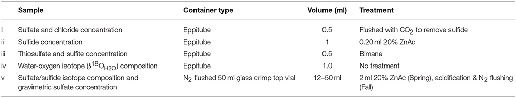
Table 1. Sampling protocol/distribution.

All isotope analyses were carried out at the stable isotope laboratory of the Department of Earth Sciences at ETH Zurich. All isotope values are reported according to the standard delta notation, relative to VSMOW for oxygen and VCDT for sulfur isotope measurements.

For the water-oxygen isotope analysis, 0.5 ml of sample was pipetted into a flat bottomed vial, the vial sealed and flushed with a CO₂/He mixture and allowed to equilibrate on a shaker at room temperature for at least 12 h. For every 10 samples, two in-house standards (WS2011, δ¹⁸O = −0.59‰; MW2011, δ¹⁸O = 12.23‰) were inserted. After equilibration between CO₂ headspace and the water sample, the samples and standards were transferred to a Thermo Scientific GasBench^® equipped with an auto-sampler and connected to a ThermoFinnigan Delta V Plus^® isotope ratio mass spectrometer (IRMS), with which the oxygen isotope composition of the CO₂ from the sample headspace was analyzed. The standard deviation (1σ) for replicate measurements of the two laboratory standards for water-oxygen isotope analysis was < 0.1‰.

Oxygen isotope analysis of sulfate was done by continuous-flow isotope ratio mass spectrometry with a high temperature thermal conversion elemental analyzer, specifically a ThermoFinnigan TCEA^®/Conflo IV^®/Delta V Plus^® IRMS combination. Approximately 0.3 mg of BaSO₄ samples and associated standards (NBS-127, IAEA-SO-5, and IAEA-SO-6) were weighed into silver capsules and carefully sealed. Samples and standards were then loaded into a Zero-Blank autosampler connected to the TCEA^® and run. The standard deviation (1σ) for replicate measurements of a laboratory standard for oxygen isotope analysis of solid material was < 0.5‰.

Sulfur isotope analysis was also done by continuous-flow isotope ratio mass spectrometry, but now coupled with a high temperature combustion elemental analyzer, specifically a Eurovector CNS analyzer^® connected to a ThermoFinnigan Delta V^® IRMS. For the determination of the sulfur isotope compositions of pure substances, i.e., BaSO₄ samples and standards, or Ag₂S samples and standards, 0.2–0.4 mg were weighed into tin capsules with an approximately equal amount of vanadium pentoxide (V₂O₅). The sulfur isotope measurements of BaSO₄ were calibrated with reference materials NBS-127 (δ³⁴S = +21.1‰), IAEA-SO-5 (δ³⁴S = 0.49‰), and IAEA-SO-6 (δ³⁴S = −34.1‰). The standard deviation (1σ) for replicate measurements of a BaSO₄ laboratory standard was < 0.5‰. The sulfur isotope measurements of Ag₂S were calibrated with reference materials IAEA-S-2 (previously called NZ2, δ³⁴S = 22.6‰) and IAEA-S-3 (δ³⁴S = −32.5‰). The standard deviation (1σ) for replicate measurements of a Ag₂S laboratory standard was < 0.3‰.

Results and Discussion

Sulfate Concentrations

The sulfate concentration profiles from sediment cores taken in Spring and Fall are very similar. There is good general agreement between the sulfate concentrations measured by ion chromatography and by gravimetric method based on the weight of barium sulfate precipitates, even at very low sulfate concentrations, such as for the deep sulfate pool in the Fall core (Table 2; Figure 2). Reproducibility of sulfate concentrations via gravimetric method based on multiple control samples is better than 0.02 mM (1 sd). In the absence of direct methane concentration measurements on the cores in this study, we consider the SMT to begin after sulfate concentrations drop below 1 mM and assign the base of the SMT to the depth directly above the deep sulfate pool. We define the deep sulfate pool as sulfate in the sediment column below the SMT where the sulfur and oxygen isotope composition of sulfate shows no clear depth trend and which begins at approximately a depth of 190 cm for both cores. For the Spring core, between a depth of 150 and 205 cm there is a discrepancy between sulfate concentrations determined by ion chromatography and the gravimetric method (Figure 2B). The good agreement between the gravimetric method and ion chromatography results from the Fall sampling campaign demonstrates that the gravimetric method does not systematically underestimate sulfate concentrations. The higher sulfate concentrations determined by ion chromatography in Spring could be due to incomplete sulfide removal during sampling and subsequent oxidation to sulfate. During the Spring campaign, sulfide was stripped by bubbling pure carbon dioxide gas through the sample. In the SMT, the sulfide peak concentrations can reach 5.5 mM (Holmkvist et al., 2011). Due to enhanced rates of sulfate reduction coupled to AOM, the pore-water pH is well buffered by the production of bicarbonate and carbonate ions. These circumstances may have led to incomplete sulfide removal by the carbon dioxide stripping in this portion of the sediment column. Irrespective of the reasons for the elevated sulfate concentrations determined by ion chromatography, we refer to the values determined by gravimetric method in the discussion of samples from the SMT and the deep sulfate zone, as the oxygen and sulfur isotope values were determined on the very same sub-samples.

TABLE 2

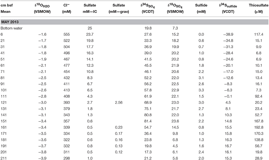
Table 2. Concentration and isotope data for the Spring campaign.

FIGURE 2

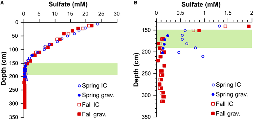
Figure 2. (A) Sulfate concentration profiles for cores from Spring and Fall 2013 and (B) detailed profiles for the low sulfate concentration range. For the Spring core, there is a discrepancy between sulfate concentration measurements by ion chromatographic and gravimetric method. Error on the sulfate concentrations determined by ion chromatography is ±15% and better than ±0.02 mM by gravimetric method. The green band represents the SMT.

Chloride Concentrations and Oxygen Isotope Composition of Water

Chloride concentrations decreased with depth, with a steeper gradient for the core taken in the Spring as compared to the core from the Fall (Figure 3A). A similar trend is observed for the oxygen isotope composition of water (Table 2). A cross plot of chloride vs. the oxygen isotope composition of water reveals nearly identical slopes for both the Spring and Fall (Figure 3B).

FIGURE 3

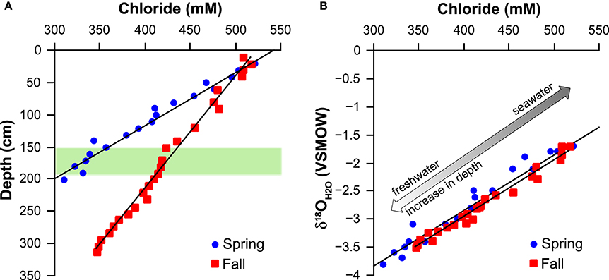
Figure 3. (A) Chloride concentration vs. depth. Intercept at chloride = 0 indicates a freshwater source at 441 and 908 cm for Spring and Fall, respectively. (B) Chloride concentration vs. oxygen isotope composition of pore water intercept at chloride = 0 yields an oxygen isotope composition of the underlying freshwater source of ~ −7‰ (−6.78‰ Spring and −6.96‰ Fall). The green band represents the SMT.

Linear extrapolation of the chloride gradients to zero concentration locates the depth of a potential freshwater interface to 441 cm depth for the core taken in Spring and 908 cm depth for the core taken in Fall. Both cores were taken at the approximately same position (i.e., within a distance of maximally 100 m). Beneath the Holocene marine sediments of Aarhus Bay is a buried landscape of till and sand that was formed by the glaciers toward the end of the last ice age, before the marine transgression took place some 9000 years ago. At site M1, where the cores were taken, a transition from terrestrial to marine sediments is observed at ca. 10 m depth, but the topography of this paleo-landscape can be highly variable over short lateral distances. Thus, the uppermost terrestrial sand layers may be the source of a freshwater intrusion to the overlaying marine deposits and the differences between the chloride and oxygen isotope profiles between the two sampling campaigns may be the result of a small deviation in coring location. A plot of the chloride vs. the oxygen isotope composition of pore water indicates that the fresh water source is likely the same for the Spring and Fall cores, with a tentative groundwater oxygen isotope composition of ~ −7‰ (Figure 3B). This value is close to the oxygen isotope composition of meteoric water in Denmark (−8‰; Jørgensen and Holm, 1994) and to the isotope composition of water from two wells at Stautrup Waterworks near Aarhus (−7.95 to −8.65‰; Jørgensen and Holm, 2012).

Concentration of Sulfite and Thiosulfate

The concentrations of sulfite and thiosulfate were only determined for the Spring core. Sulfite could be detected, but was below the quantifiable level of 0.5 μM. Thiosulfate concentrations fall in a range from 7 to 16 μM for most of the top 100 cm of the core, and show a peak of 193 μM between 150 and 185 cm, below which they drop to 29 μM at the bottom of the core at 211 cm (Table 2).

Concentration and Sulfur Isotope Composition of Sulfide

The concentration of sulfide scatters strongly for both the Spring and Fall core samples (Tables 2, 3). We attribute this to the degassing of sulfide during sample processing, particularly to the loss of sulfide when the sediment is placed in the pore water press that is being vigorously flushed with N₂ to minimize potential sulfide oxidation. The sulfur isotope composition of sulfide does not appear to be affected by this loss. Values increase from the top of the cores (−38.9‰, Spring and −31.2‰, Fall) to heaviest values at 190 cm depth (16.7‰ for the Spring and 17.7‰ for the Fall core). Sulfide-sulfur isotope compositions then show a slight drop to lower values toward the bottom the cores (15.3, 15.5‰ for Spring and Fall, respectively). Notably, the sulfur isotope composition of sulfide below the SMT is fairly close to the isotope composition of bottom water sulfate at station M1 (19.8‰).

TABLE 3

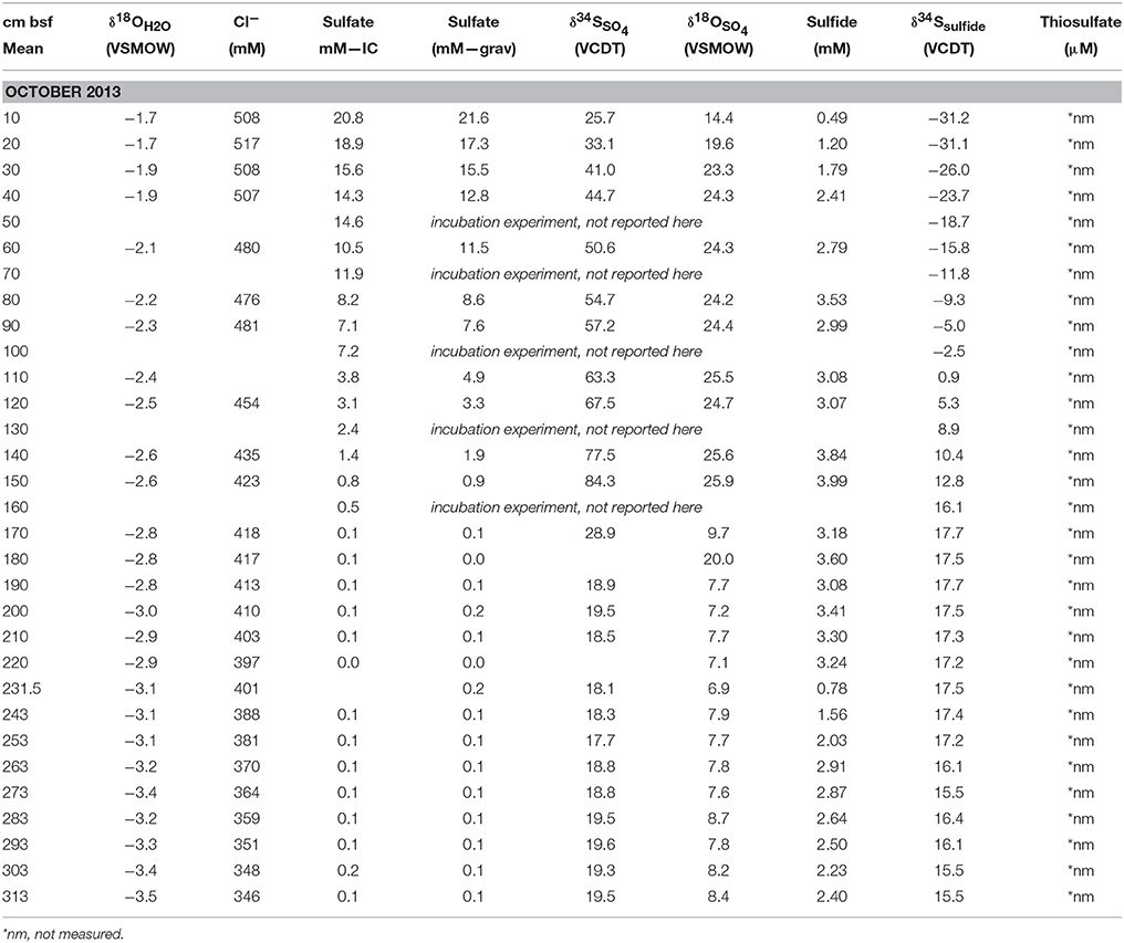
Table 3. Concentration and isotope data for the Fall campaign.

Sulfur and Oxygen Isotope Composition of Sulfate

In the top 150 cm of the sediment, the sulfur isotope values of sulfate show gradual relative enrichment of the heavy isotopes with depth. The δ³⁴S increased from 20‰ at the sediment surface to >80‰ where sulfate dropped to < 1 mM in the SMT (Tables 2, 3; Figure 4A). The sulfur isotope offset between sulfate and sulfide was remarkably constant, with an average value of 66 ± 2‰ for the Spring core and 65 ± 4‰ for the Fall core. The δ¹⁸O of sulfate increased from 7.3‰ in the bottom water to about 15‰ in the top 0–10 cm and approached a plateau below 30 cm that is close to the oxygen isotope equilibrium fractionation between water and sulfate (Figure 4B; Fritz et al., 1989; Zeebe, 2010).

FIGURE 4

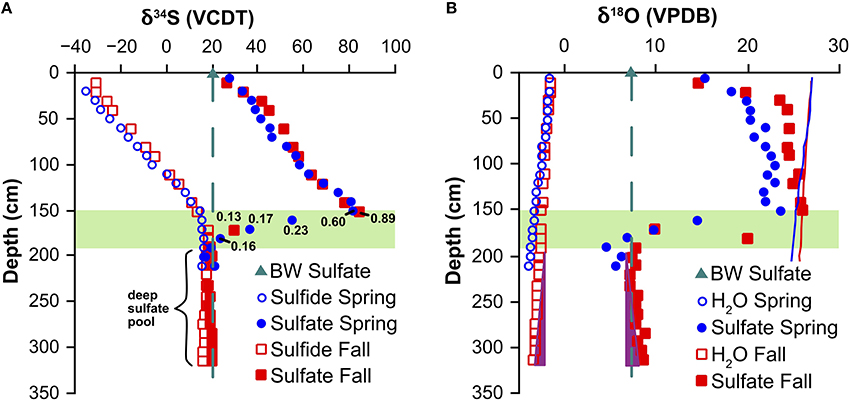
Figure 4. (A) Sulfur and (B) oxygen isotope trends for sulfate, sulfide, and pore-water. The samples below a depth of 190 cm are designated as “deep sulfate pool,” whereas samples in between a sediment depth of 150 and 190 cm are considered to belong to the lower part of the SMT. The dark green triangle and dashed line represent the seawater sulfate isotope composition. The solid blue and red line (B) are the predicted sulfate-oxygen isotope composition at equilibrium with water calculated from Fritz et al. (1989). Purple triangles (B) indicate oxygen isotope trends for water and sulfate do not correlate. The green band represents the SMT.

Just beneath the maximum values reached in the SMT, the δ³⁴S and δ¹⁸O of sulfate dropped steeply to values that are remarkably close to the isotope composition of seawater sulfate at the sampling site (δ³⁴S = 19.8‰ and δ¹⁸O = 7.3‰). For the samples obtained in the Spring, the oxygen isotope values fell slightly below the values for seawater sulfate. Sulfate concentrations below the SMT remained in a narrow range of 0.04–0.18 mM (Figure 2B) and showed a rather uniform sulfur and oxygen isotope composition. We designate this pool as the “deep sulfate pool,” starting at approximately 190 cm depth and expanding down through the methanic zone. It is interesting to note that while the oxygen isotope values of the pore water decreased with depth (Figure 4B), there was no corresponding pattern in the δ¹⁸O of sulfate.

Potential Sampling Artifacts

With regards to potential artifacts during sampling of pore water from the methanic zone, there are two major concerns. First, a minor contamination with seawater sulfate can have detrimental consequences for the interpretation of the data, and second, sulfide can oxidize to sulfate if exposed to oxygen once the core is retrieved, also adversely affecting data quality (for an example see Raven et al., 2016). During the sampling campaign in Spring 2013, four whole-round core samples were taken from a well aligned core retrieved in parallel with the core used for all pore water concentration and isotope data. Two whole-round core samples were taken from within the main sulfate reduction zone (S44: 110–120 cm and S43: 140–150 cm depth) and two from below the SMT (S42: 170–180 cm and S41: 195–205 cm depth) to test 1) the potential contamination with seawater sulfate and 2) the potential auto-oxidation of sulfide to sulfate during pore-water extraction. The following protocol documents the various steps:

1) The 10-cm long whole-round core samples were cut with the sediment remaining in the core liner. The exposed sediment at the top and bottom was then generously sprayed with ¹⁸O-labeled deionized water with an oxygen isotope composition of 4800‰. The whole-round core samples were then tightly wrapped in plastic film, secured with tape, and remained for at least 48 h in the cold room.

2) After a minimum of 48 h, a Rhizon^® sampler was inserted through the film and pushed into the center of the sample segment. A volume of ~1.5 ml was then removed for sulfate concentration measurements and oxygen isotope analysis of water.

3) Immediately after Rhizon^® sampling, the sediment was prepared for pore-water extraction. First, the top film cover was removed, and the sediment partially extruded by pushing on the still film-sealed bottom of the whole round section. Approximately 2 cm sediment was extruded, sliced off with a clean knife, and set aside for further processing. The same procedure was used to extract sediment from the bottom of the core. A clean section of plastic film was used to push the remaining sample down and partially out of the bottom of the section where again, 2 cm of sediment was sliced off with a clean knife, and added to the “top” sediment. The combined top and bottom 2 cm sub-samples were kept in a plastic container vigorously flushed with N₂ gas until pore-water extraction with a pore-water press at a later stage.

4) Without any delay, the remaining sediment core was extruded onto a clean surface, and the sides of the core (~2 cm) were scraped off and placed in a plastic container that was vigorously flushed with N₂ gas before pore-water extraction with a pore-water press at a later stage. Typically, the outside of the sediment core that was previously in contact with the core liner, showed a discoloration, presumably a result of oxidation.

5) Next, the freshly exposed center of the sediment core was generously sprayed with the ¹⁸O-labeled deionized water (δ¹⁸O = 4800‰) so that the entire surface was wet. The core sample was then immediately placed into a pore-water press flushed with N₂ gas. The first 3–5 ml of pore water was discarded, followed by collection of ~25 ml into a capped serum bottle (previously amended with 2 ml 20% zinc acetate and flushed with N₂), followed by collection of ~8 ml of pore-water in a plastic syringe for sulfate concentration and other analyses, and finally the remaining pore water (typically another ~25 ml) into the capped serum bottle. This back-and-forth procedure was chosen to avoid collecting predominantly ¹⁸O labeled water, which is likely to be more quickly extruded by the press than interstitial pore water in the initial phase of extraction.

6) Subsequent to processing the center sample, pore-water was extracted from the “Bottom & Top” and “Side” samples with the pore-water press. The first 3–5 ml of pore water was discarded, followed by collecting ~8 ml of pore water in a separate container for sulfate concentration and other analyses. The remaining pore-water (typically < 20 ml due to small amount of sediment) was transferred into a capped serum bottle that was previously amended with 2 ml 20% zinc acetate and flushed with N₂.

It is important to note that placing samples in a plastic container that is vigorously flushed with N₂ gas will remove some H₂S, which is easily detectable as sulfide smell. Further loss of H₂S occurs when the sample is placed into the pore water press, which is also flushed with N₂. Consequently, severe underestimation of sulfide concentrations has to be expected when this method is employed. The sulfur isotope composition of collected sulfide, however, is not expected to be significantly altered by this loss.

Two objectives were pursued with the experiments with the heavily isotopically labeled water (δ¹⁸O = 4800‰). The first objective was to obtain a quantitative estimate of potential contamination with sulfate when a core segment was for more than 48 h in contact with a thin layer of seawater with a concentration of 28 mM sulfate. Such a scenario may occur if the diameter of the sediment core is smaller than the inner diameter of the core liner, leaving a thin gap which would allow for a contact of seawater with the exterior of the sediment core (Figure 5). As pore water squeezing is a time consuming process, sulfate from this thin film of seawater would have time to diffuse into the samples. The samples obtained with a Rhizon^® inserted into the center of the sediment core segments and the samples obtained from the sides of the cores can provide an estimate of the extent of such a contamination with sulfate because they reveal how much ¹⁸O-labeled water penetrated deeply into the sediment from the top and bottom of the core segment within a time frame of over 48 h. These estimates represent a worst-case scenario because the molecular diffusion of sulfate ions is slower than self-diffusion of H₂₁₈O (D_sulfate = 0.56 * 10⁻⁵ cm² s⁻¹ in seawater at 4°C; Iversen and Jørgensen, 1985); D_{water: self-diffusion} = 1.26 * 10⁻⁵ cm² s⁻¹ in water at 4°C; Holz et al., 2000). Moreover, isotopically labeled water might be entrained from the top of the core when the Rhizon^® is stuck into the center of the core. Finally, sediment from the side of the core is prone to exposure to isotopically labeled water that seeps down- and upward along the core liner. The approximate mixing contribution of pristine water (1 − x) relative to isotopically labeled water (x) can be calculated as follows:

$\begin{array}{rc}\text{x}=1-({\delta }^{18}{\text{O}}_{\text{mixture}}-{\delta }^{18}{\text{O}}_{\text{label}})∕({\delta }^{18}{\text{O}}_{\text{pristine}}-{\delta }^{18}{\text{O}}_{\text{label}}).& \left(1\right)\end{array}$

FIGURE 5

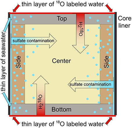
Figure 5. Cross-section of whole-round core segment depicting potential contamination with sulfate from seawater and the experimental procedure with ¹⁸O labeled water to quantify potential sulfate penetration.

If we now assume that pristine pore water was sulfate-free, the found value of x can be multiplied with the assumed concentration of sulfate contaminant (i.e., 28 mM), which yields the hypothetical concentration in the contaminated sample (Table 4). Our calculated “worst-case” potential contamination with sulfate from seawater falls in a range of 0.03–0.11 mM, with an average of 0.07 mM. Such a contamination could constitute a major portion of sulfate in the deep sulfate pool, i.e., it could reach 50% of the total sulfate concentration within 48 h. Initially, the results from our Spring studies where we focused on the effects of auto-oxidation indicated that an extended pore water extraction protocol would not adversely affect our results. However, in light of the fact that the deep sulfate samples for the Fall core were extracted between 48 and 86 h after core retrieval, the potential for contamination with sulfate by diffusion is high.

TABLE 4

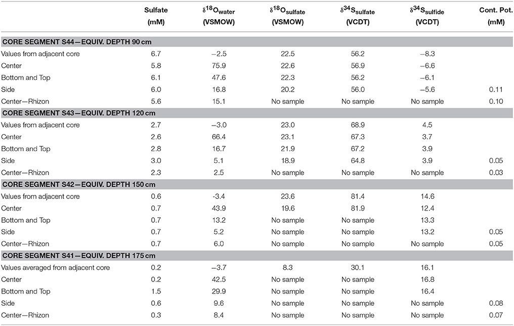
Table 4. Results of sampling artifact experiments.

The second objective was to explore if auto-oxidation of sulfide to sulfate after core retrieval may have affected the sulfate concentration and the isotope data. Oxidation of sulfide by atmospheric oxygen would occur along the same diffusion path as the introduced ¹⁸O labeled water. The oxygen isotope composition of water leaves a strong imprint on the isotope composition of sulfate generated by sulfide oxidation even if atmospheric oxygen (O₂) is the oxidant (e.g., see Müller et al., 2013 for role of sulfite as an intermediate in sulfide oxidation, and Taylor et al., 1984 for minimum oxygen incorporation from water into produced sulfate during wet/dry pyrite weathering). Because sulfide is also depleted in ³⁴S relative to the sulfate, one would further expect negative shifts in the sulfur isotope composition of sulfate. The experiments with core segment S43, which was stored in the cold room for more than 48 h demonstrates the effects of sulfide oxidation (Table 4). The sulfur and oxygen isotope composition of sulfate from the center of the sample shows similar values as for the sample from the adjacent core, which was fully processed in < 48 h after coring. However, the measurements from the top and bottom, as well as the side of core segment S43 are different from its center. Particularly, the side of the core shows a higher sulfate concentration (3.0 mM) than the center (2.6 mM), and a lower oxygen and sulfur isotope composition of sulfate (δ¹⁸O = 18.9‰, δ³⁴S = 64.8‰) than the sulfate from the center (δ¹⁸O = 23.1‰, δ³⁴S = 67.3‰). This observation indicates that sulfide from the side, top and bottom of the core segment was oxidized, resulting in the addition of isotopically light sulfate. However, it appears the center of the core remained unaffected by this oxidation. Pore water squeezing of the core center of core segment S43, which was preceded by spraying of the freshly exposed center of the sediment with the ¹⁸O-labeled deionized water (δ¹⁸O = 4800‰) resulting in an oxygen isotope composition of the extracted water of 66.4‰, did not yield sulfate enriched in ¹⁸O, indicating that sulfide oxidation to sulfate during pore water squeezing is negligible. This finding is corroborated by the results from the experiment with core segment S42 which was also stored for more than 48 h, where the isotope composition of sulfate from the center of the core (δ¹⁸O = 19.6‰, δ³⁴S = 81.9‰) is close to the isotope composition of an adjacent core (δ¹⁸O = 23.6‰, δ³⁴S = 81.9‰) which was processed in less than 24 h (Table 4).

In conclusion, the experiments with ¹⁸O-isotopically labeled water show that auto-oxidation of sulfide during core storage and pore water squeezing is unlikely to impact our measurements. However, these experiments do not shed light on the potential for sulfide oxidation in subsequent sample preparation steps, as exemplified by the discrepancy between sulfate concentrations determined by ion chromatography and gravimetric method in Spring. Obviously, potential contamination with seawater sulfate is a concern. A contamination with 4 μl of bottom water per 1 ml of sulfate-free pore water would be sufficient to result in an apparent sulfate concentration of 0.1 mM with an isotopic composition of seawater.

Interpretation

A simple explanation of our data could therefore be that in situ there is no deep sulfate pool but that the observed sulfate is the result of an artifact caused by contamination with seawater sulfate. In this scenario, one could assume that sulfate is entirely consumed by sulfate reduction within the SMT, and that the steep drop in sulfate-sulfur and -oxygen isotope composition from the center of the SMT to the lower limit of the SMT is the result of mixing of contaminant seawater sulfate and the very last remainder of original sulfate (Table 5; Figure 4). We can quantitatively explore this scenario in more detail for the samples at a depth of 161, 171 (Spring core), and 170 cm (Fall core). The very last remainder of original sulfate is likely to have an oxygen isotope composition close to the oxygen isotope equilibrium between sulfate and water (isotopic difference ~25‰), whereas the sulfur isotope composition of sulfate is unknown. The isotope composition of contaminant sulfate from seawater is known (δ³⁴S_cont = 19.8‰ and δ¹⁸O_cont = 7.3‰). Using these values and the sulfate concentration and isotope composition of the mixture between original sulfate and contaminant, one can quantify the hypothetical amount of contaminant sulfate, and determine the sulfur isotope composition of original sulfate (Table 5, for derivations of equations, see Appendix). On the average, the concentration of contaminant present is 0.13 mM sulfate, which is a good match to the sulfate concentrations in the deep sulfate pool (0.14 mM for the Spring core and 0.10 mM for the Fall core). The inferred sulfur isotope composition of the original sulfate for the investigated samples falls in a range of 90–138‰. Such strong enrichments in ³⁴S are not outside of the realm of possibilities, considering that the estimated amounts of residual sulfate can be as low as 0.02 mM and that the sulfur isotope composition might display a Rayleigh distillation trend. The implication of attributing the observed signatures to a mixture of residual sulfate and contamination would be that sulfate reduction coupled to the anaerobic oxidation of methane strongly fractionates sulfur isotopes even at very low sulfate concentrations, consistent with recent modeling results for sulfur isotope fractionation during microbial sulfate respiration (Wing and Halevy, 2014).

TABLE 5

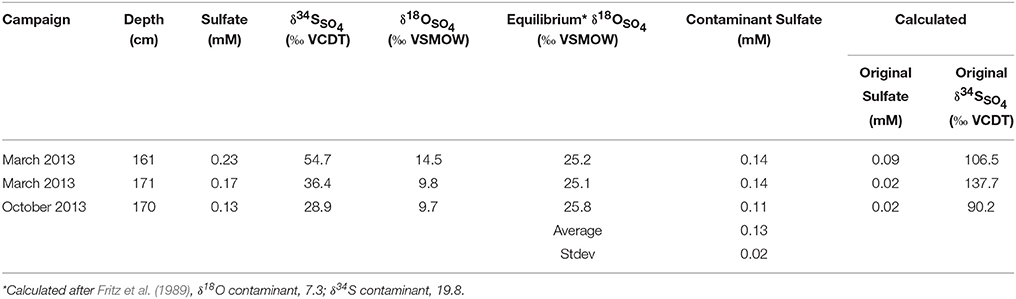
Table 5. Contaminant mixing table.

The explanation that the observed sulfate concentration and isotope patterns from sediments below of the SMT are the result of contamination with seawater is compelling, and in our point of view at this stage, the most prudent interpretation of the data. However, there are inconsistencies in this scenario that must be addressed. A major inconsistency is that the oxygen isotope composition of sulfate for the four deepest samples for the Spring core are distinctly lighter than the oxygen isotope composition of seawater sulfate (average for δ¹⁸O_sulfate of 5.7 vs. 7.3‰) and that one of these four sample shows a sulfate-sulfur isotope composition that is lighter than the isotope composition of seawater sulfate (17.3 vs. 19.8‰; Figure 4). These values cannot be the result of contamination with seawater sulfate and the clustering of the sulfur and oxygen isotope data make it unlikely that they could be the result of analytical error, i.e., we do not observe such variation in values for the entire deep sulfate pool for the Fall core. Hence, one would have to postulate that they are the result of auto-oxidation of sulfide—but there is no evidence that would support that this process is of importance for the time between coring and pore water extraction. Essentially, one would have to argue that auto-oxidation of sulfide after pore water extraction was the cause for the observed concentration and isotope patterns for sulfate obtained from the deepest part of the Spring core, whereas the contamination with sulfate was the cause of the patterns observed for the Fall core. As the sampling campaigns are not fully identical, one cannot rule out this possibility. In the Spring, sulfide was captured using a zinc acetate solution to precipitate zinc sulfide, separated from sulfate by vacuum filtration, followed by the acidification of the filtrate and removal of any residual sulfide with a CO₂ gas stream. The earliest extracted samples from at and below of the SMT that were fixed with zinc acetate remained in the cold room for up to 100 h within the sealed, nitrogen-flushed serum bottles before filtration. In the Fall, sulfide was immediately removed directly after pore water collection by acidification of the filtrate and flushing with a CO₂ gas stream. It would be curious and interesting find that one of the standard techniques to prevent sulfide oxidation—the fixation as zinc sulfide—yields artifacts, whereas immediate removal of sulfide by acidification is more reliable.

Another fact for consideration is that there is no increase in sulfate concentration observable for samples that were extracted toward the end of the pore water extraction process in Fall (Figure 6). Sulfate concentrations from deep in the sediment core are low, but variable indicating no relationship with regards to the time of sample processing or the potential for vertical diffusion and mixing. If there was contamination with seawater sulfate it would have had to occur early in the sampling campaign and then remain fixed throughout sample processing.

FIGURE 6

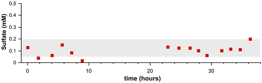
Figure 6. Sulfate concentrations (red squares) from samples extracted by pore water press during a time frame of 36 h. They gray band represents ±1 sd of the average sulfate concentration for all sub-SMT samples in the Fall core. The sediment core (Fall 2013) was retrieved 2 days prior to when pore water pressing started (t = 0).

If it is Not an Artifact, Then What?

Being aware of these provisos, it is worth searching for an explanation of the persistent presence of sulfate and the sulfate-sulfur and -oxygen isotope composition below the SMT for the case where the observance of low concentrations of sulfate is not a result of an artifact. The concentration and isotope gradients between sulfate present in the SMT and the sulfate at the base of the SMT demonstrates that this pool does not represent “left over” sulfate that was not consumed during anaerobic oxidation of methane coupled to sulfate reduction. This isotopic shift can be achieved if the sulfate removed by sulfate reduction coupled to the anaerobic oxidation of methane is simultaneously replenished by either (i) an oxidative process, (ii) admixture of brackish water, or (iii) release of sulfate from a solid phase.

It is conceivable that the availability and reactivity of sulfide oxidants, as well as availability of substrates for microbial sulfate reduction, is uniform in the sediments that host the deep sulfate pool. This would explain why sulfate concentrations and sulfur isotope signatures in this closed oxidative-reductive sulfur turnover tend to be uniform as well. The remarkable similarity between the sulfur isotope composition of deep sulfate (δ³⁴S = 18.9‰) and seawater (δ³⁴S = 19.8‰) may be rooted in the fact that sulfide produced at the SMT approaches the sulfur isotope composition of seawater sulfate (δ³⁴S of up to 17.5‰). As this sulfide diffuses downward into the deep sulfate pool, it can be oxidized to sulfate, a process that causes only a slight enrichment in the sulfur isotope composition (e.g., Fry et al., 1988; Balci et al., 2007; Brabec et al., 2012). Alternatively, it could be speculated that production of isotopically light sulfate at the base of the SMT is the result of polysulfide disproportionation. Polysulfides occur in direct proportion to the free sulfide concentration (Holmkvist et al., 2014) and may be produced by the activity of ANME archaea during sulfate reduction coupled to the anaerobic oxidation of methane at the SMT (Milucka et al., 2012). These polysulfides may be disproportionated throughout the sediment column (Fossing and Jørgensen, 1990). The presence of thiosulfate at and below the SMT highlights that sulfur species that can be disproportionated into sulfate and sulfide are indeed available (Table 2). One observation casts doubt on a scenario where newly formed sulfate in the methanic zone coincidentally yields the same oxygen isotope composition as seawater sulfate from Aarhus Bay. The water-oxygen isotope composition of the pore water continuously decreases within the methanic zone, from −2.8‰ at 170 cm depth to −3.5‰ at 313 cm depth. No such trend is observable for the oxygen isotope composition of sulfate over the same depth interval (Figure 4).

An appealing alternative scenario is an admixture of seawater and groundwater from a permeable sediment layer beneath the SMT, because it presents an explanation for the similarity in the isotope composition of deep sulfate and the bottom water collected from the sampling site (δ³⁴S = 19.8‰, δ¹⁸O = 7.3‰) and for the decoupling of the oxygen isotope composition of deep sulfate from the oxygen isotope composition of water which continues to decrease with depth (Figure 4). The homogeneous, muddy sediments found in the cores indicate that it is unlikely that a permeable layer exists in close proximity to the base of the SMT. However, it could be speculated that a slight change in the slope in the chloride profile at depth (ca. 160 cm in the Spring core and 190 cm in the Fall core) may indicate local admixture of brackish water with low sulfate and chloride content. Lateral advection of sulfate through a broad sediment zone below the base of the SMT (that coincides with the location of the deep sulfate pool) with slightly enhanced permeability can be excluded based on the continuous gradient in the chloride concentration and oxygen isotope composition of water. This leaves the option of an admixture of seawater from a source below the sampled sediment profile. The decrease in both the chloride concentration and oxygen isotope composition of water with increasing depth are testimony of the existence of such an aquifer and agrees with descriptions of the sediment in Aarhus Bay (e.g., sandy sediments—previous topography at around 10 m depth; Jensen and Bennike, 2009). It is possible that the water in such an aquifer is brackish due to mixing of seawater with freshwater. In this scenario, the near-constant sulfate concentration and isotope profile from the bottom of the cores to the base of the SMT would be explained as the result of diffusive mixing in absence of any sulfate production or consumption.

Finally, dissolution of marine barite due to low sulfate concentrations (e.g., Riedinger et al., 2006) or release of carbonate-associated sulfate due to carbonate recrystallization catalyzed by the production of CO₂ associated with methanogenesis (Meister et al., 2011) could contribute to the stability of sulfate concentrations and isotope signatures in the deep sulfate pool (Figure 4). However, it must be noted that barite dissolution in sulfate-free seawater would yield a sulfate concentration < 20 μM, which is 5–10 fold smaller than the observed sulfate concentrations in the deep sulfate pool. With regards to the release of carbonate-associated sulfate in the Aarhus Bay sediments, carbonate is present in the form of mollusk shells throughout the sediment column (Holmkvist et al., 2011). Sulfate release from carbonates during recrystallization is difficult to assess, as this process involves simultaneous carbonate dissolution and re-precipitation, which may not be detected in concentration profiles of dissolved inorganic carbon, calcium, or magnesium. Nevertheless, it is evident that sulfate loss from carbonates occurs during this process (Staudt and Schoonen, 1995).

Curiously, all of the above arguments demand that in the deep sulfate zone sulfate reduction does not fractionate sulfur and oxygen isotopes, because the latter would drive the isotope values of sulfate heavy. This is problematic, as it is known that sulfate concentrations between 0.1 and 0.2 mM do not preclude microbial sulfate reduction (Holmkvist et al., 2011; Tarpgaard et al., 2011). Sulfur isotope fractionation during classical microbial sulfate reduction at low sulfate concentrations can be low (Habicht et al., 2002), for an alternative view see Canfield et al. (2010a). Recently, a modeling-based argument convincingly demonstrated that sulfur isotope fractionation by microbial sulfate reduction can be large (up to equilibrium isotope fractionation) at low sulfate concentration and low sulfate reduction rates (Wing and Halevy, 2014). If the argument that sulfur isotope fractionation by sulfate reduction is negligible in the deep sulfate zone holds, the oxygen isotope effects should be negligible as well, because both processes are linked by the reversibility of the sulfate reduction pathway (Brunner et al., 2005, 2012). Alternatively, sulfate consuming organisms in the methanic zone may employ sulfate reduction pathways that do not fractionate sulfur isotopes, for example pathways that are similar to sulfate assimilation or yet to-be elucidated sulfate reduction pathways inferred for ANME (Milucka et al., 2012), however, it needs to be noted that the phylogenetic diversity of sulfate reducers in the methanic zone are rather similar to those in the lower part of the sulfate zone (Leloup et al., 2009).

Conclusions

Avoiding artifacts in the extraction of sulfate from sulfidic low-sulfate pore water remains a challenge. Our sampling strategy overcomes the challenges related to sulfate production from sulfide auto-oxidation, but did not resolve all issues with regards to contamination with seawater sulfate. Consequently, it may be prudent to first assume that the sulfate detected in Aarhus Bay sediments retrieved below the SMT is a result of contamination with sea water sulfate. Isotope mass balance calculations indicate that in this scenario, the sulfur isotope compositions in the bottom part of the SMT could be as high as 138‰ at residual sulfate concentrations as low as 0.02 mM. The implication of this finding is that sulfate reduction coupled to the anaerobic oxidation of methane strongly fractionates sulfur isotopes also at very low sulfate concentrations.

However, not all of the data for sulfate retrieved from the base or below of the SMT can be satisfactorily explained as result of contamination with seawater sulfate. The sulfate-oxygen isotope composition of the four deepest samples for the Spring campaign is lighter than the oxygen isotope composition of seawater sulfate, which is indicative for an oxidative process that either occurs in situ or as sampling artifact (i.e., auto-oxidation of reduced sulfur species). Our experiments indicate that auto-oxidation of reduced sulfur species does not pose a major issue for the stage between storage of the core in the cold room and pore water extraction. The main difference in sampling procedures between Spring and Fall is that the pore water in the Spring samples was amended with zinc acetate as to fix sulfide as zinc sulfide, a step that was omitted in Fall. For future studies of low-sulfate/high-sulfide environments this observation implies that the classic approach to fix sulfide as zinc sulfide may not be advisable.

Casting aside prudence, it is worthwhile to consider the implications if the data from the base and from below the SMT are not the result of artifacts. For the Spring core one would have to conclude that new sulfate is generated at the base of the SMT. Potential processes could be oxidative sulfur cycling with ferric iron (Riedinger et al., 2014; Sivan et al., 2014) or a yet unknown oxidant. For the Fall core one would need to find an answer to the question of how sulfate at depth can have a sulfur and oxygen isotope signature that is remarkably similar to seawater sulfate. Release of carbonate associated sulfate during carbonate recrystallization and dissolution of marine barite could provide such a signature, however, there is no quantitative assessment of the importance of these processes at this point. With regards to the elucidation of sulfur cycling at the base and below of the SMT much remains to be explored. It is known that organisms with the capability to reduce sulfate exist and thrive in methanic sediments (Leloup et al., 2007). At least, our data hint that oxidative sulfur cycling occurs at the base of the SMT providing encouragement to the further investigation of this process.

A lesson learned from our sampling campaigns is that contamination with seawater sulfate remains a major challenge whereas auto-oxidation of reduced sulfur species can be kept to a minimum using appropriate sampling protocols. Core-processing takes time and additional steps should be taken to prevent contamination with seawater during processing. One option to overcome contamination with seawater sulfate would be to take two parallel cores from the same site. One core could then be immediately sampled with Rhizon^® samplers that are stuck in the center of the core segments. At the least, the pore water obtained in this way can be analyzed for sulfate concentrations. With a combination of elaborate sulfur extraction techniques (Arnold et al., 2014) and high sensitivity isotope analysis by multi-collector ICPMS (Paris et al., 2013; Lin et al., 2014) it might even be possible to measure the sulfur isotope composition of sulfate. However, in light that barite dissolution in sulfate-free seawater would yield a sulfate concentration < 20 μM researchers must brace themselves for extremely low sulfate concentrations for sulfur and oxygen isotope analyses. Another lesson learned is that the concentration of sulfate and the sulfur isotope composition of sulfate are valuable tools for the interpretation of the data, but the most revealing information comes from the oxygen isotope composition of sulfate and water. This is in so far critical as high sensitivity oxygen isotope analysis by multi-collector ICPMS is not available. Unfortunately, for gas source isotope ratio mass spectrometry, much larger sulfate samples are needed, and this is where a second, parallel core would be helpful. The outer sediment of such a core would need to be removed as soon as possible after core retrieval to avoid contamination with seawater. More sophisticated alternatives such as freezing of core segments or freeze coring could be employed.

There are also new avenues in the exploration of cryptic sulfur cycling in marine sediments. The measurement of barite dissolution and carbonate recrystallization rates could help quantifying sulfate input from these sources, quantitative modeling of oxygen isotope exchange between sulfate and water in the main sulfate zone based on sulfur and oxygen isotope profiles (Wortmann et al., 2007) could provide insight if sulfur oxidation may also be important in this zone, and long-term studies with stable isotope tracers (in or ex situ) could provide direct evidence for the presence or absence of cryptic sulfur cycling.

Author Contributions

All authors listed, have made substantial, direct and intellectual contribution to the work, and approved it for publication.

Conflict of Interest Statement

The authors declare that the research was conducted in the absence of any commercial or financial relationships that could be construed as a potential conflict of interest.

Acknowledgments

We thank Stefano Bernasconi, Stewart Bishop, and Madalina Jaggi (ETH Zurich) for assistance with isotope analyses. We also thank Jeanette Pedersen and Karina Bomholt Henriksen (Aarhus University), for analytical work and technical support. We thank the Max Planck Institute for Marine Microbiology in Bremen for assistance with the concentration analysis of thiosulfate and sulfite and for lending us the pore water press. We are especially grateful to Captain Torben Vang and the crew of the RV Tyra of Aarhus University for outstanding support during the Aarhus Bay sampling campaigns. We thank our two reviewers for their encouraging and insightful comments. The research was funded by the Danish National Research Foundation and the European Research Council (ERC) Advanced Grant, MICROENERGY (grant n° 294200), awarded to BJ under the EU 7th FP. This work was supported by start-up funds for BB by the University of Texas at El Paso.

References

Arnold, G. L., Brunner, B., Müller, I. A., and Røy, H. (2014). Modern applications for a total sulfur reduction distillation method - what's old is new again. Geochem. Trans. 15:4. doi: 10.1186/1467-4866-15-4

PubMed Abstract | CrossRef Full Text | Google Scholar

Balci, N., Shanks, I. I. I., Mayer, B., and Mandernack, K. W. (2007). Oxygen and sulfur isotope systematics of sulfate produced by bacterial and abiotic oxidation of pyrite. Geochim. Cosmochim. Acta 71, 3796–3811. doi: 10.1016/j.gca.2007.04.017

CrossRef Full Text | Google Scholar

Bao, H. (2006). Purifying barite for oxygen isotope measurement by dissolution and reprecipitation in a chelating solution. Anal. Chem. 78, 304–309. doi: 10.1021/ac051568z

PubMed Abstract | CrossRef Full Text | Google Scholar

Bishop, T., Turchyn, A. V., and Sivan, O. (2013). Fire and brimstone: the microbially mediated formation of elemental sulfur nodules from an isotope and major element study in the Paleo-Dead Sea. PLoS ONE 8:e75883. doi: 10.1371/journal.pone.0075883

PubMed Abstract | CrossRef Full Text | Google Scholar

Brabec, M. Y., Lyons, T. W., and Mandernack, K. W. (2012). Oxygen and sulfur isotope fractionation during sulfide oxidation by anoxygenic phototrophic bacteria. Geochim. Cosmochim. Acta 83, 234–251. doi: 10.1016/j.gca.2011.12.008

CrossRef Full Text | Google Scholar

Brunner, B., Bernasconi, S. M., Kleikemper, J., and Schroth, M. H. (2005). A model for oxygen and sulfur isotope fractionation in sulfate during bacterial sulfate reduction processes. Geochim. Cosmochim. Acta 69, 4773–4785. doi: 10.1016/j.gca.2005.04.017

CrossRef Full Text | Google Scholar

Brunner, B., Einsiedl, F., Arnold, G. L., Müller, I., Templer, S., and Bernasconi, S. M. (2012). The reversibility of dissimilatory sulphate reduction and the cell-internal multi-step reduction of sulphite to sulphide: insights from the oxygen isotope composition of sulphate. Isotopes Environ. Health Stud. 48, 33–54. doi: 10.1080/10256016.2011.608128

PubMed Abstract | CrossRef Full Text | Google Scholar

Canfield, D. E., Farquhar, J., and Zerkle, A. L. (2010a). High isotope fractionations during sulfate reduction in a low-sulfate euxinic ocean analog. Geology 38, 415–418. doi: 10.1130/G30723.1

CrossRef Full Text | Google Scholar

Canfield, D. E., Stewart, F. J., Thamdrup, B., Brabandere, L. D., Dalsgaard, T., Delong, E. F., et al. (2010b). A cryptic sulfur cycle in oxygen-minimum–zone waters off the chilean Coast. Science 330, 1375–1378. doi: 10.1126/science.1196889

PubMed Abstract | CrossRef Full Text | Google Scholar

Fossing, H., and Jørgensen, B. B. (1990). Oxidation and reduction of radiolabeled inorganic sulfur compounds in an estuarine sediment, Kysing Fjord, Denmark. Geochim. Cosmochim. Acta 54, 2731–2742. doi: 10.1016/0016-7037(90)90008-9

CrossRef Full Text | Google Scholar

Fritz, P., Basharmal, G. M., Drimmie, R. J., Ibsen, J., and Qureshi, R. M. (1989). Oxygen isotope exchange between sulphate and water during bacterial reduction of sulphate. Chem. Geol. 79, 99–105. doi: 10.1016/0168-9622(89)90012-2

CrossRef Full Text | Google Scholar

Fry, B., Ruf, W., Gest, H., and Hayes, J. M. (1988). Sulfur isotope effects associated with oxidation of sulfide by O2 in aqueous solution. Chem. Geol. 73, 205–210. doi: 10.1016/0168-9622(88)90001-2

PubMed Abstract | CrossRef Full Text | Google Scholar

Habicht, K. S., Gade, M., Thamdrup, B., Berg, P., and Canfield, D. E. (2002). Calibration of sulfate levels in the Archean Ocean. Science 298, 2372–2374. doi: 10.1126/science.1078265

PubMed Abstract | CrossRef Full Text | Google Scholar

Holmkvist, L., Ferdelman, T. G., and Jørgensen, B. B. (2011). A cryptic sulfur cycle driven by iron in the methane zone of marine sediment (Aarhus Bay, Denmark). Geochim. Cosmochim. Acta 75, 3581–3599. doi: 10.1016/j.gca.2011.03.033

CrossRef Full Text | Google Scholar

Holmkvist, L., Kamyshny, A. Jr., Brüchert, V., Ferdelman, T. G., and Jørgensen, B. B. (2014). Sulfidization of lacustrine glacial clay upon Holocene marine transgression (Arkona Basin, Baltic Sea). Geochim. Cosmochim. Acta 142, 75–94. doi: 10.1016/j.gca.2014.07.030

CrossRef Full Text | Google Scholar

Holz, M., Heil, S. R., and Sacco, A. (2000). Temperature-dependent self-diffusion coefficients of water and six selected molecular liquids for calibration in accurate 1H NMR PFG measurements. Phys. Chem. Chem. Phys. 2, 4740–4742. doi: 10.1039/B005319H

CrossRef Full Text | Google Scholar

Iversen, N., and Jørgensen, B. B. (1985). Anaerobic methane oxidation rates at the sulfate-methane transition in marine sediments from Kattegat and Skagerrak (Denmark). Limnol. Oceanogr. 30, 944–955. doi: 10.4319/lo.1985.30.5.0944

CrossRef Full Text | Google Scholar

Jensen, J. B., and Bennike, O. (2009). Geological setting as background for methane distribution in Holocene mud deposits, Århus Bay, Denmark. Cont. Shelf Res. 29, 775–784. doi: 10.1016/j.csr.2008.08.007

CrossRef Full Text | Google Scholar

Johnston, D. T., Gill, B. C., Masterson, A., Beirne, E., Casciotti, K. L., Knapp, A. N., et al. (2014). Placing an upper limit on cryptic marine sulphur cycling. Nature 513, 530–533. doi: 10.1038/nature13698

PubMed Abstract | CrossRef Full Text | Google Scholar

Jørgensen, N. O., and Holm, P. M. (1994). “Isotope studies (18O/16O, D/H and 87Sr/86Sr) of saline groundwater in Denmark,” in Future Groundwater Resources at Risk (Helsinki Conference, FGR 94), (Helsinki: IAHS).

Google Scholar

Jørgensen, N. O., and Holm, P. M. (2012). Strontium-isotope studies of chloride-contaminated groundwater, Denmark. Hydrogeol. J. 3, 52–57. doi: 10.1007/s100400050066

CrossRef Full Text | Google Scholar

Leloup, J., Fossing, H., Kohls, K., Holmkvist, L., Borowski, C., and Jørgensen, B. B. (2009). Sulfate-reducing bacteria in marine sediment (Aarhus Bay, Denmark): abundance and diversity related to geochemical zonation. Environ. Microbiol. 11, 1278–1291. doi: 10.1111/j.1462-2920.2008.01855.x

PubMed Abstract | CrossRef Full Text

Leloup, J., Loy, A., Knab, N. J., Borowski, C., Wagner, M., and Jørgensen, B. B. (2007). Diversity and abundance of sulfate-reducing microorganisms in the sulfate and methane zones of a marine sediment, Black Sea. Environ. Microbiol. 9, 131–142. doi: 10.1111/j.1462-2920.2006.01122.x

PubMed Abstract | CrossRef Full Text | Google Scholar

Lin, A.-J., Yang, T., and Jiang, S.-Y. (2014). A rapid and high-precision method for sulfur isotope δ34S determination with a multiple-collector inductively coupled plasma mass spectrometer: matrix effect correction and applications for water samples without chemical purification. Rapid Commun. Mass Spectrom. 28, 750–756. doi: 10.1002/rcm.6838

CrossRef Full Text | Google Scholar

Meister, P., Gutjahr, M., Frank, M., Bernasconi, S. M., Vasconcelos, C., and McKenzie, J. A. (2011). Dolomite formation within the methanogenic zone induced by tectonically driven fluids in the Peru accretionary prism. Geology 39, 563–566. doi: 10.1130/G31810.1

CrossRef Full Text | Google Scholar

Mikucki, J. A., Pearson, A., Johnston, D. T., Turchyn, A. V., Farquhar, J., Schrag, D. P., et al. (2009). A contemporary microbially maintained subglacial ferrous “Ocean.” Science 324, 397–400. doi: 10.1126/science.1167350

PubMed Abstract | CrossRef Full Text

Milucka, J., Ferdelman, T. G., Polerecky, L., Franzke, D., Wegener, G., Schmid, M., et al. (2012). Zero-valent sulphur is a key intermediate in marine methane oxidation. Nature 491, 541–546. doi: 10.1038/nature11656

PubMed Abstract | CrossRef Full Text | Google Scholar

Müller, I. A., Brunner, B., and Coleman, M. (2013). Isotopic evidence of the pivotal role of sulfite oxidation in shaping the oxygen isotope signature of sulfate. Chem. Geol. 354, 186–202. doi: 10.1016/j.chemgeo.2013.05.009

CrossRef Full Text | Google Scholar

Paris, G., Sessions, A. L., Subhas, A. V., and Adkins, J. F. (2013). MC-ICP-MS measurement of δ34S and Δ33S in small amounts of dissolved sulfate. Chem. Geol. 345, 50–61. doi: 10.1016/j.chemgeo.2013.02.022

CrossRef Full Text | Google Scholar

Raven, M. R., Sessions, A. L., Fischer, W. W., and Adkins, J. F. (2016). Sedimentary pyrite δ34S differs from porewater sulfide in Santa Barbara Basin: proposed role of organic sulfur. Geochim. Cosmochim. Acta 186, 120–134. doi: 10.1016/j.gca.2016.04.037

CrossRef Full Text | Google Scholar

Riedinger, N., Formolo, M. J., Lyons, T. W., Henkel, S., Beck, A., and Kasten, S. (2014). An inorganic geochemical argument for coupled anaerobic oxidation of methane and iron reduction in marine sediments. Geobiology 12, 172–181. doi: 10.1111/gbi.12077

PubMed Abstract | CrossRef Full Text | Google Scholar

Riedinger, N., Kasten, S., Gröger, J., Franke, C., and Pfeifer, K. (2006). Active and buried authigenic barite fronts in sediments from the Eastern Cape Basin. Earth Planet. Sci. Lett. 241, 876–887. doi: 10.1016/j.epsl.2005.10.032

CrossRef Full Text | Google Scholar

Sivan, O., Antler, G., Turchyn, A. V., Marlow, J. J., and Orphan, V. J. (2014). Iron oxides stimulate sulfate-driven anaerobic methane oxidation in seeps. Proc. Natl. Acad. Sci. U.S.A. 111, E4139–E4147. doi: 10.1073/pnas.1412269111

PubMed Abstract | CrossRef Full Text | Google Scholar

Staudt, W. J., and Schoonen, M. A. A. (1995). “Sulfate incorporation into sedimentary carbonates,” in Geochemical Transformations of Sedimentary Sulfur ACS Symposium Series (American Chemical Society), 332–345. doi: 10.1021/bk-1995-0612.ch018

CrossRef Full Text | Google Scholar

Tarpgaard, I. H., Røy, H., and Jørgensen, B. B. (2011). Concurrent low- and high-affinity sulfate reduction kinetics in marine sediment. Geochim. Cosmochim. Acta 75, 2997–3010. doi: 10.1016/j.gca.2011.03.028

CrossRef Full Text | Google Scholar

Taylor, B. E., Wheeler, M. C., and Nordstrom, D. K. (1984). Stable isotope geochemistry of acid mine drainage: experimental oxidation of pyrite. Geochim. Cosmochim. Acta 48, 2669–2678. doi: 10.1016/0016-7037(84)90315-6

CrossRef Full Text | Google Scholar

Teske, A. (2010). Cryptic links in the Ocean. Science 330, 1326–1327. doi: 10.1126/science.1198400

PubMed Abstract | CrossRef Full Text | Google Scholar

Wing, B. A., and Halevy, I. (2014). Intracellular metabolite levels shape sulfur isotope fractionation during microbial sulfate respiration. Proc. Natl. Acad. Sci. U.S.A. 111, 18116–18125. doi: 10.1073/pnas.1407502111

PubMed Abstract | CrossRef Full Text | Google Scholar

Wortmann, U. G., Chernyavsky, B., Bernasconi, S. M., Brunner, B., Böttcher, M. E., and Swart, P. K. (2007). Oxygen isotope biogeochemistry of pore water sulfate in the deep biosphere: dominance of isotope exchange reactions with ambient water during microbial sulfate reduction (ODP Site 1130). Geochim. Cosmochim. Acta 71, 4221–4232. doi: 10.1016/j.gca.2007.06.033

CrossRef Full Text | Google Scholar

Zeebe, R. E. (2010). A new value for the stable oxygen isotope fractionation between dissolved sulfate ion and water. Geochim. Cosmochim. Acta 74, 818–828. doi: 10.1016/j.gca.2009.10.034

CrossRef Full Text | Google Scholar

Appendix

The oxygen isotope mass balance,

$\begin{array}{l}{\delta }^{18}{\text{O}}_{\text{mix}}=\text{x}•{\delta }^{18}{\text{O}}_{\text{cont}}+(1-\text{x})•{\delta }^{18}{\text{O}}_{\text{eq}}\end{array}$

is rearranged to yield the value for the relative contribution of the contaminant (x), according to

$\begin{array}{l}\text{x}=({\delta }^{18}{\text{O}}_{\text{mix}}-{\delta }^{18}{\text{O}}_{\text{eq}})∕({\delta }^{18}{\text{O}}_{\text{cont}}-{\delta }^{18}{\text{O}}_{\text{eq}}).\end{array}$

The absolute amount of contaminant equals x•conc_mix, and the amount of original sulfate equals (1 − x)• conc_mix. The sulfur isotope mass balance,

$\begin{array}{l}{\delta }^{34}{\text{S}}_{\text{mix}}=\text{x}•{\delta }^{34}{\text{S}}_{\text{cont}}+(1-\text{x})•{\delta }^{34}{\text{S}}_{\text{orig}}\end{array}$

is then rearranged to yield the sulfur isotope composition of original sulfate,

$\begin{array}{l}{\delta }^{34}{\text{S}}_{\text{orig}}=({\delta }^{34}{\text{S}}_{\text{mix}}-x•{\delta }^{34}{\text{S}}_{\text{cont}})∕(1-\text{x}).\end{array}$