The Changing Impact of Snow Conditions and Refreezing on the Mass Balance of an Idealized Svalbard Glacier

1. Introduction

During the most recent decades, Arctic temperatures have increased at an amplified rate compared to the global mean (ACIA, 2005; IPCC, 2013), which has been ascribed to retreating sea-ice cover and resulting ice—atmosphere feedbacks (Serreze and Francis, 2006; Bintanja and van der Linden, 2013). Additionally, precipitation in the Arctic has increased in recent decades in response to atmospheric moistening (Min et al., 2008; Zhang et al., 2012). Increases in both precipitation and temperature in the Arctic are projected to accelerate during the remainder of the twenty-first century (Bengtsson et al., 2011; Bintanja and Selten, 2014).

The climate on the high-Arctic archipelago of Svalbard, located at the northern end of the Atlantic warm water current, is highly sensitive to variability and trends in winter-time sea-ice extent (Divine and Dick, 2006; Day et al., 2012), as well as changes in atmospheric circulation patterns (Hanssen-Bauer and Førland, 1998). Observed temperatures at Svalbard Airport, Longyearbyen, between 1898–2012 show a marked positive mean trend of 0.26°C decade⁻¹ (Nordli et al., 2014). A strong seasonal contrast prevails in observed temperature trends with markedly more pronounced warming in winter/spring than in summer (Førland et al., 2011; Bintanja and van der Linden, 2013; Nordli et al., 2014). Observational precipitation records in Svalbard since the early and mid-twentieth century reveal weakly positive trends, with low significance due to substantial local-scale and instrumental uncertainty (Førland and Hanssen-Bauer, 2000). Projections for Svalbard, based on empirical downscaling, indicate a continued modest precipitation increase and a three times higher warming rate up to the year 2100 than observed over the last 100 years (Førland et al., 2011).

Changing temperature and precipitation conditions affect the energy and mass balance of Svalbard glaciers. Estimates of the multi-decadal mass balance of all Svalbard glaciers, disregarding frontal ablation, are close to zero with values ranging between −0.05 m w.e. a⁻¹ for 1979–2013 (Lang et al., 2015) and 0.08 m w.e. a⁻¹ for 1957–2014 (Østby et al., in review). Frontal calving of tide-water glaciers is a substantial mass loss term and has been estimated at −0.18 m w.e. a⁻¹ for 2000–2006 (Blaszczyk et al., 2009). Altogether, recent warming has enhanced glacier thinning, which has been estimated at −0.59 m a⁻¹ for 1961–2005, based on airborne/satellite altimetry for six glaciers around Svalbard (James et al., 2012). As a dynamic response to glacier thinning, glaciers in Svalbard have shrunk by 7% of their total area during the past 30 years for a sample of around 400 glaciers (Nuth et al., 2013).

The interaction between a glacier surface, the atmosphere above and the underlying snow/firn determines the climatic mass balance. The climatic mass balance is defined as the sum of the surface mass balance, due to surface accumulation and ablation, and the internal mass balance (Cogley et al., 2011). Rising temperature induces more surface melting, but the timing and rate of melt water discharge depends strongly on the presence and state of seasonal snow and firn. Snow acts as a buffer against mass loss due to its mirroring effect on solar radiation, which reduces heat absorption and surface melt, and because it can store percolating melt water in either solid (refrozen) or liquid form. Refreezing of percolating and stored water in snow and firn contributes significantly to the mass balance of glaciers and ice sheets and has a pronounced impact on subsurface temperature and density (Jania et al., 1996; Wright et al., 2007; Reijmer et al., 2012). It is generally most pronounced in accumulation zones and peaks in spring when first melt enters the cold snow pack and in fall when the cold wave induces refreezing of stored liquid water.

While there has been much focus on the direct mass-retaining effect of refreezing (e.g., Pfeffer et al., 1991; Reijmer et al., 2012), there has been considerably less attention for the role of indirect effects after refreezing. The primary mass balance effect of refreezing is to retain melt/rain water in refrozen form, thereby reducing the fraction of melt/rain water that runs off. At the same time heat release and solid mass retention by refreezing affect the thermodynamic state and stratigraphy of the snow pack, thereby affecting the conductive heat flux and potentially the surface albedo, which in turn influence surface melt and runoff. A detailed assessment of the impact of refreezing on the mass balance of glaciers requires a coupled treatment of surface and snow processes, and is highly relevant for modeling melt and discharge of Arctic glaciers.

In a warming climate, higher melt rates lead to firn densification and thinning, ultimately causing a retreat of the perennial snow cover to higher elevations. Rapid near-surface densification in lower accumulation zones in south-west Greenland (Machguth et al., 2016) and western Svalbard (Van Pelt and Kohler, 2015) are manifestations of this. Shrinking accumulation zones (1) amplify melt rates in summer due to increased bare-ice exposure (ice—albedo feedback), and (2) reduce the potential for melt water retention by refreezing. Both effects reduce the buffering role of snow and firn against mass loss in a warming climate (e.g., Van Angelen et al., 2013; Van Pelt and Kohler, 2015).

Our aim with this study is to investigate the changing state of snow and firn conditions in Svalbard and its impact on glacier mass loss in a past, present and future climate (1984–2104). Numerical simulations are done with a coupled surface energy balance—firn model (EBFM; Van Pelt et al., 2012; Van Pelt and Kohler, 2015), on a synthetic elevation-dependent grid. We attempt to simulate evolving surface and snow/firn conditions along the centerline of an idealized inland Svalbard glacier. Such a set-up facilitates an analysis with a focus on the process understanding and helps to identify the role of feedback mechanisms. The constructed climate forcing relies on variability from the Svalbard Airport meteorological station, a seasonally-dependent future projection scenario (Førland et al., 2011), and observation-based elevation lapse rates. The model, climate forcing and experimental setup are described in Section 2. Model results are analyzed and discussed in Section 3. Finally, conclusions and recommendations are given in Section 4.

2. Methods

2.1. Model

A coupled energy balance—firn model (EBFM) is used to perform simulations on a synthetic elevation dependent grid. Here, we briefly summarize the main qualitative model aspects; for a more complete overview of the coupled model and its implementation, see Van Pelt et al. (2012) and Van Pelt and Kohler (2015) and references therein. The model has previously been used to study the mass balance and firn evolution of Nordenskiöldbreen in central Svalbard (Van Pelt et al., 2012, 2013, 2014; Vega et al., 2016), and Kongsvegen and Holtedahlfonna in western Svalbard (Christianson et al., 2015; Van Pelt and Kohler, 2015).

Driven by meteorological fields, at every model time-step a surface energy balance model sums the heat fluxes at the surface in order to determine the surface temperature and the energy involved in melting:

$\begin{array}{l}{Q}_{\mathrm{\text{melt}}}=Q_{\mathrm{\text{sw}}}+Q_{\mathrm{\text{lw}}}+Q_{\mathrm{\text{turb}}}+Q_{\mathrm{\text{ghf}}}+Q_{\mathrm{\text{rain}}},& (1)\end{array}$

where Q_melt is the energy available for melt, Q_sw is the net shortwave radiation, Q_lw is the net longwave radiation, Q_turb is the turbulent heat exchange by the latent and sensible heat flux, Q_ghf is the conductive ground heat flux, and Q_rain is the energy supplied by rainfall. The surface temperature is limited to 0°C, any excess energy results in melting of the surface layer (Q_melt > 0). Formulations of the individual energy fluxes can be found in Klok and Oerlemans (2002); a qualitative description of the individual fluxes is given below.

In order to solve the surface energy balance climate input of air temperature, relative humidity, cloud cover and precipitation is required by this model. Cloud cover, temperature and relative humidity affect the incoming shortwave radiation, which depends on the top-of-atmosphere radiation, atmospheric transmissivity and the grid orientation (Klok and Oerlemans, 2002). Reflected shortwave radiation is determined by the albedo, following a snow depth and age dependent formulation (Oerlemans and Knap, 1998). Incoming longwave radiation is formulated as a function of cloud cover, relative humidity and air temperature (Konzelmann et al., 1994), while the Stefan-Boltzmann law for a black body describes emitted longwave radiation. The description of turbulent sensible and latent heat exchange uses bulk equations by Oerlemans and Grisogono (2002), requiring climate input of air temperature and relative humidity, respectively. The ground heat flux represents conduction between the surface skin layer and the underlying snow/ice and can take both signs depending on the near-surface temperature gradient. Finally, the heat supplied by rainfall depends on air temperature and is generally a small term. The model distinguishes between snow and rainfall by using a gradual (linear) transition from snow to rain between air temperatures of 0.5 and 2.5°C; hence, at a temperature of 1.5°C precipitation consists of 50% rain and snow (Van Pelt et al., 2012).

Energy and mass exchange at the surface provides an upper boundary condition for the subsurface model, tracking the evolution and vertical distribution of temperature, density and water content. The multi-layer subsurface model is based on Reijmer and Hock (2008) and later modified and extended by Van Pelt et al. (2012). The energy consumed in melting the surface may be released again as latent heat below the surface when percolating or stored water refreezes in snow or firn layers. The subsurface model solves the thermodynamic equation, accounting for heat conduction and refreezing:

$\begin{array}{ll}\rho c_p(T)\frac{\partial T}{\partial t}=\frac{\partial }{\partial z}\left(\kappa (\rho )\frac{\partial T}{\partial z}\right)+\frac{RL}{d},& (2)\end{array}$

where T is the layer temperature, ρ the layer density, c_p(T) the specific heat capacity, κ(ρ) the effective conductivity, R the refreezing rate (kg m⁻² s⁻¹), L the latent heat of fusion and d the layer thickness. The subsurface model additionally solves the densification equation, considering refreezing and gravitational packing of the snow G(ρ, T) (Ligtenberg et al., 2011):

$\begin{array}{ll}\frac{\partial \rho }{\partial t}=G(\rho ,T)+\frac{R}{d}.& (3)\end{array}$

Vertical water transport and refreezing is simulated using a bucket scheme (Greuell and Konzelmann, 1994; Reijmer and Hock, 2008; Van Pelt et al., 2012). Storage of percolating water occurs in two forms: (1) on its way down a small amount of water is held in temperate layers against capillary forces (irreducible water), and (2) water accumulates on top of impermeable ice to form a layer of slush water, thereby filling the remaining pore space. Runoff occurs at the firn-ice transition and is instantaneous in the case of bare-ice exposure and according to a slope-dependent time-scale for standing slush water within the snow-pack (Reijmer and Hock, 2008).

The climatic mass balance is a direct measure for mass changes resulting from the interaction of atmosphere, glacier surface and the underlying snow/firn (Cogley et al., 2011). It is therefore effectively a measure for mass change at and below the surface, down to the base of the snow or firn pack (if present). The climatic mass balance is defined here as the sum of mass gain, through precipitation and condensation/riming, and mass loss, through runoff and evaporation/sublimation. Refreezing may act as a buffer against mass loss where a firn/snowpack is present, as it reduces the amount of melt water that runs off. In our experiments the climatic mass balance is assumed to be equal to the sum of mass changes above the base of the model domain at 15–20 m depth; any potential refreezing below this depth is regarded as negligible.

2.2. Climate Forcing

2.2.1. Temporal Variability

In order to run the coupled model, meteorological input of precipitation, air temperature, cloud cover and relative humidity is required at a sub-daily temporal resolution. Meteorological data of the above parameters, collected at the coastal meteorological station at Svalbard Airport at 28 m a.s.l., Longyearbyen (Norwegian Meteorological Institute, eKlima.no) are used as time-series for 1975–2014. Six-hourly observations of temperature, cloud cover and relative humidity were interpolated to the 3-h model resolution, whereas observed 12-h precipitation sums were split into 3-h bins. The average temperature between 1 September 1975 and 31 August 2014 was equal to −5.0 °C, precipitation summed to 191 mm a⁻¹, mean relative humidity was equal to 74%, and average cloud cover was 64%.

Time-series of winter (DJF), spring (MAM), summer (JJA) and autumn (SON) mean observed temperature and precipitation between 1975–2014 (first 39 years in Figure 1), show a clear inhomogeneity in observed seasonal temperature trends. Over the observation period 1975–2014, winter warming (2.2°C decade⁻¹) exceeds summer warming (0.5°C decade⁻¹) by a factor of four. Much stronger winter than summer warming, referred to as Arctic winter warming (AWW), is one of the key features of Arctic Amplification and has been ascribed to the retreat of sea ice and the resulting ice—atmosphere feedbacks (Serreze and Francis, 2006; Bintanja and van der Linden, 2013).

FIGURE 1

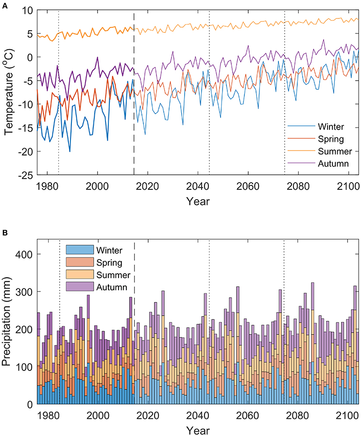
Figure 1. Time-series of observed and projected winter (DJF), spring (MAM), summer (JJA) and autumn (SON) temperature (A) and precipitation (B) for the period 1975–2104.

Førland et al. (2011) used the NorACIA (Norwegian Arctic Climate Impact Assessment) regional climate model, with input from six atmosphere ocean general circulation model (AOGCM) simulations for a range of emission scenarios (A1B, A2, and B2), to simulate the past (1961–1990) and future (2071–2100) climate in the Svalbard region. The ensemble results present seasonal temperature and precipitation trends between 1961–1990 and 2071–2100, yielding linear seasonal temperature trends for Svalbard Airport of 1.0 (DJF), 0.6 (MAM), 0.3 (JJA) and 0.5°C decade⁻¹ (SON) and precipitation trends of 0.4 (DJF), 2.6 (MAM), 1.0 (JJA), and 1.9 % decade⁻¹ (SON) (Førland et al., 2011).

In addition to seasonal inhomogeneity in warming, at intra-seasonal time-scales (days to weeks) cold spells are found to warm faster than warm spells. This is apparent when comparing trends per season of above-average (upper 50%) and below-average (lower 50%) temperatures in the 1975–2014 Svalbard Airport record, as shown in Figure 2. Below-average temperatures were found to increase 1.5 (DJF), 2.1 (MAM), 2.1 (JJA), and 1.6 (SON) times faster than above-average temperatures, which indicates more rapid warming of cold spells for all seasons.

FIGURE 2

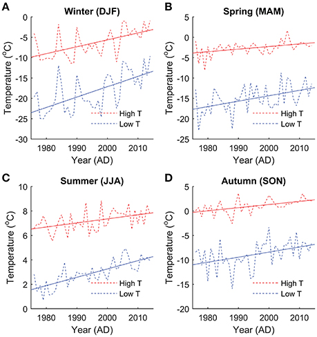
Figure 2. Time-series of winter (DJF; A), spring (MAM; B), summer (JJA; C) and autumn (SON; D) temperature at Svalbard Airport for the period 1975–2104, averaged per year for above-average (upper 50%; dashed red line) and below-average (lower 50%; dashed blue line) values.

In order to extend the 1975–2014 climate forcing into the future, we first repeat variability of temperature, precipitation, cloud cover and relative humidity, observed at Svalbard Airport between 1984–2014, three times to cover the period 2014–2104. In a next step, we impose seasonal trends in temperature and precipitation, according to Førland et al. (2011). Finally, for the temperature projection we additionally account for the aforementioned inhomogeneity in warming of cold and warm spells, as observed in the Svalbard Airport record. More specifically, the following steps are applied to generate future time-series for temperature, precipitation, cloud cover and relative humidity:

1. Observed 3-h time-series of temperature, precipitation, cloud cover and relative humidity during the 30-year reference period (1984–2014), are repeated three times into the future to cover the 90-year period from 1 September 2014 to 31 August 2104.

2. Seasonal trends of temperature and precipitation in Førland et al. (2011) are imposed on the future time-series. Seasonally inhomogeneous trends are already present in the reference climate (1984–2014) and thus also within the repeated future 30-year blocks. Therefore, for every season corrections for seasonally inhomogeneous warming are applied per 30-year block, i.e., an entire 30-year block is shifted to conform with the change applicable for the midpoint of the 30-year period. After trend application, mean seasonal temperatures between 2015 and 2104 increase by 8.6 (DJF), 5.2 (MAM), 2.3 (JJA), and 4.6 °C (SON), and seasonal precipitation rates rise by 3 (DJF), 23 (MAM), 9 (JJA), and 17% (SON), in line with projections in Førland et al. (2011).

3. Inhomogeneity of warming of cold and warm spells within seasons during the observational period (Figure 2), is assumed to persist in a future climate. A time-dependent temperature correction is implemented by multiplying the seasonal trends applied in step 2 by a time-dependent function, which is <1 for above-average temperatures and >1 for below-average temperatures. The function is equal to 1+ΔT(t)*C_T, where ΔT(t) is the temperature deviation at time-step t from the 30-year running seasonal mean, and C_T (in K⁻¹) is a seasonally-dependent coefficient, which represents the fractional change of the seasonal trend per degree temperature deviation from the 30-year running seasonal mean. With seasonal values of C_T of −0.034 (DJF), −0.057 (MAM), −0.160 (JJA), and −0.048 K⁻¹ (SON) continuation of the observed inhomogeneity at Svalbard Airport between 1975–2014 (Figure 2) is assured in the future temperature scenario.

The resulting time-series of seasonally averaged temperature and precipitation for 1975–2104 are shown in Figure 1. The projected climate scenario includes changes in temperature and precipitation variability. Stronger winter than summer warming reduces the magnitude of the annual temperature cycle (Figure 1A). Additionally, more pronounced warming of cold than warm spells leads to a reduction of short-term (intra-seasonal) temperature variability. The latter is also responsible for the decrease of inter-annual variability in seasonal temperatures (Figure 1A), since relatively warm seasons (compared to the 30-year mean) will experience a weaker warming trend than relatively cold seasons. Finally, seasonal precipitation trends cause the magnitude of individual precipitation events to increase, while the frequency of precipitation events remains unchanged in the projected climate.

The above described approach to generate meteorological time-series provides a strong alternative to using climate output from a single future realization of a RCM, which is prone to substantial uncertainty given the generally large spread between individual RCM projection runs. The current approach also has some limitations. While we incorporate expected changes in the magnitude of temperature and precipitation variability, no potential long-term changes in the frequency and distribution of weather events are accounted for. For example, an increased frequency of heavy-precipitation events in the Northern hemisphere has been suggested (Min et al., 2011), although a recent analysis of extreme precipitation events in Svalbard reveals no significant trends over the most recent decades (Serreze et al., 2015). Furthermore, we do not account for potential trends in cloud cover and relative humidity, due to a current lack of constraints of long-term trends of these variables. This is believed to have a minor impact on the presented results, since (summer) temperature and precipitation are assumed to be the dominant factors influencing the climatic mass balance and snow/firn development. To test sensitivity of the model results to different climate scenarios, a set of climate sensitivity experiments is performed (Section 3.5).

2.2.2. Elevation Dependence

Experiments are performed on an elevation-dependent model grid, representing the centerline of a typical inland Svalbard glacier. Constructed time-series of temperature, precipitation, cloud cover and relative humidity (Section 2.2.1) apply at sea-level elevation. An elevation-dependent climate forcing is constructed by applying lapse rates for temperature and precipitation, using values typical for Svalbard glaciers. Based on previous estimates of temperature lapse rates in Svalbard which range between −0.0040°C m⁻¹ (Gardner et al., 2009) and -0.0066°C m⁻¹ (Nuth et al., 2012), we use a constant mean temperature lapse rate of −0.0053°C m⁻¹. We apply an average precipitation lapse rate of 0.97 mm w.e. a⁻¹ m⁻¹, based on GPR measurements in 1997–1999 in different regions on Svalbard (Sand et al., 2003; Winther et al., 2003). Winter stake balance measurements on Holtedahlfonna in western Svalbard (Baumberger, 2007; Nuth et al., 2012; Van Pelt and Kohler, 2015) and Nordenskiöldbreen in central Svalbard (Van Pelt et al., 2012, 2014) reveal that precipitation remains constant above an approximate elevation of 800–1000 m a.s.l. Based on this, we set the elevation above which the precipitation lapse rate reduces to zero at 900 m a.s.l. No elevation lapse rates were applied for relative humidity and cloud cover.

2.3. Model Setup and Experiments

Forced with 3-h climate input (Section 2.2), we perform time-dependent experiments with EBFM (Section 2.1), on a model grid covering an altitudinal range of 0–1500 m a.s.l. An altitudinal grid spacing of 25 m is used. The subsurface model uses a moving grid consisting of 200 vertical layers with a maximum layer thickness of 10 cm; depending on surface mass fluxes layers will be added or removed at the surface and base of the vertical model domain (Van Pelt and Kohler, 2015). In contrast to a fixed grid, a moving grid avoids averaging of layer properties and assures layer properties do not suffer from numerical diffusion. The model uses a 3-h time-step, except in the calculation of subsurface heat conduction, for which adaptive time-stepping is used to assure numerical stability. In the calculation of the incoming solar radiation, we assume the surface to be flat, we neglect any shading by surrounding topography, and set the geographic position to the approximate location of Longyearbyen in central Svalbard (78°12′ N, 15°26′ E). We adopt the same model parameter setup for simulating the energy balance and subsurface conditions as in Van Pelt and Kohler (2015). In Van Pelt and Kohler (2015) surface energy balance parameters have been calibrated to optimize model performance against stake and weather station data on glaciers around Kongsfjorden in western Svalbard. Calibrated constants include the aerosol transmissivity coefficient (affects incoming solar radiation), fresh snow and ice albedo (affects reflected solar radiation), emissivity exponents for clear-sky and overcast conditions (affects incoming longwave radiation), and the turbulent exchange coefficient (affecting turbulent heat exchange). Simulated subsurface density and temperature profiles have been validated against observational data in Van Pelt et al. (2014) and Van Pelt and Kohler (2015). We do not account for any glacier dynamics, i.e., zero horizontal ice flow is assumed, which implies slight potential offsets (increasing with depth) of the presented vertical profiles. Given the shallow depth of the vertical model (up to 20 m), we believe the impact of ice flow on our results is likely to be small.

Experiments performed with EBFM cover the 120-year period between 1 September 1984 and 31 August 2104. Realistic simulation of subsurface conditions in the first years of the experiments requires initialized subsurface temperature, density and water content conditions at the start of the simulations (Van Pelt et al., 2012; Van Pelt and Kohler, 2015). To generate initial conditions, we perform a spin-up procedure in which the model is looped three times over the spin-up period 1975–1984, with meteorological input at sea-level from the Svalbard Airport record and lapse rates given in Section 2.2.2. Final output of an initialization run is used as input for the next iteration. During the 27-year spin-up procedure a snow and firn pack develops and deep density, temperature and liquid water storage approach a state consistent with the mean surface forcing between 1975–1984. Final output of the third initialization run provides initial conditions for the experiments starting 1 September 1984. Long-term runs done with EBFM include a standard run, using the above-described standard model settings, and a set of sensitivity experiments, in which the model is run without refreezing (Section 3.4) and perturbed settings for the climate scenario and elevation lapse rates (Section 3.5).

3. Results and Discussion

In this section we will present results of the model experiments. We start with a discussion of the long-term subsurface evolution at a site in the lower accumulation zone (Section 3.1). Next, we present elevation profiles of the mass balance, refreezing and subsurface conditions (Section 3.2). Thereafter, the changing role of refreezing in a future climate is discussed (Section 3.3), followed by an assessment of the impact of refreezing on the mass balance and subsurface conditions (Section 3.4). Finally, we present the outcome of climate sensitivity experiments (Section 3.5).

3.1. Subsurface Evolution

Increasing melt and rain water percolation in snow and firn in a future climate impacts the subsurface thermodynamics, stratigraphy and water storage. To illustrate the consequences of ongoing and projected climate conditions on the state of snow/firn, we first focus on the simulated firn evolution for a site at an elevation of 800 m a.s.l. for the periods 2010–2014, 2040–2044, 2070–2074, and 2100–2014 (Figure 3).

FIGURE 3

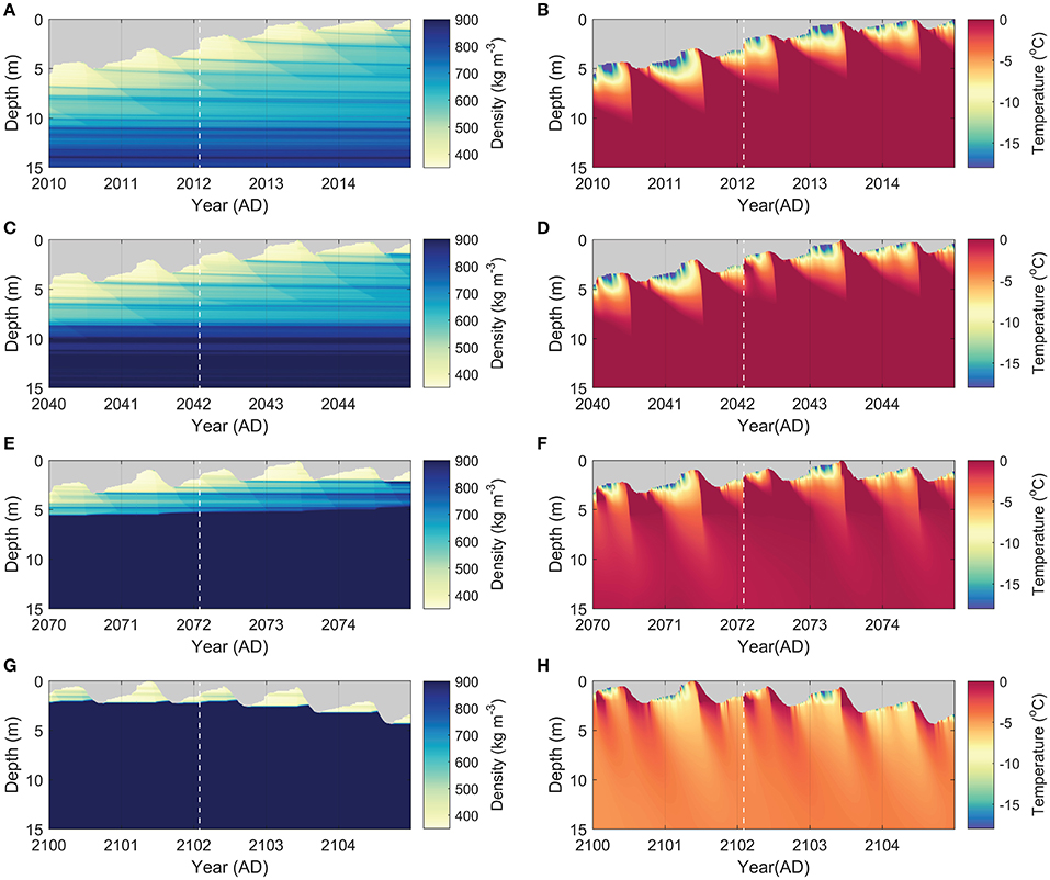
Figure 3. Subsurface density (left) and temperature (right) during the four periods 2010–2014 (A,B), 2040–2044 (C,D), 2070–2074 (E,F) and 2100–2104 (G,H) at an elevation of 800 m a.s.l. A vertical offset is applied for surface height changes with positive (negative) offsets representing surface height increase (decrease). Surface height changes are defined with respect to the base of the model domain and hence incorporate the effect of firn compaction. Depth on the y-axis is the depth with respect to the highest surface height in the 5-year period. Year labels and tick marks on the x-axis are given at 1 January of the indicated year. The white dashed line marks the onset of the rainfall event in February 2012, 2042, 2072, and 2102.

In a present-day climate, the site at 800 m a.s.l. is located in the lower accumulation zone and a thick (>10 m) firn pack is present at this elevation (Figure 3A). Heat release by refreezing of percolating water quickly removes the winter cold content at the start of the melt season (Figure 3B). Melt-freeze cycles during the melt season cause rapid near-surface densification, leading to the formation of a summer surface with elevated density every melt season (Figure 3A). At this elevation, melt water percolates throughout the firn column every summer season (Figure 3B), filling a fraction of the pore space with irreducible water. During the winter season, refreezing occurs at increasing depth as stored irreducible water gradually freezes in response to surface and firn cooling. Winter-time cooling only removes stored water by refreezing in the first meters, which causes the deeper firn to remain temperate (Figure 3B). Firn densification in the first few meters is dominated by the effect of refreezing; deeper down, gravitational settling becomes a dominant factor (Figure 3A).

In a future climate, higher summer melt rates and continued densification by refreezing and settling cause the firn pack to rapidly thin in the first decades and to disappear by the end of the twenty-first century (Figures 3C,E,G). Toward the end of the twenty-first century, this site at 800 m a.s.l. turns into ablation area, resulting in a net annual surface height lowering, absence of firn, and seasonal snow accumulation on top of the impermeable ice in winter (Figure 3G). The shallow firn—ice transition depth in the last decades limits deep water storage and refreezing, which causes deep temperatures to become non-temperate (Figure 3H). In addition to the lack of refreezing, the higher conductivity of ice compared to snow promotes more rapid winter-time cooling. Warm spells in winter and associated rainfall cause (additional) winter-time refreezing, removing part of the cold content in the upper meters. A clear example of this is seen in February 2012, 2042, 2072, and 2102; heavy winter rainfall causes deep percolation and refreezing, thereby substantially affecting subsurface temperatures (Figures 3D,F,H) and snow stratigraphy in subsequent months (Figures 3C,E,G). With winter warming being more pronounced than summer warming, the frequency of winter rainfall events is projected to increase, having a major impact on the seasonal distribution of refreezing and the thermodynamic state of snow and firn, as will be further discussed in Section 3.3.

3.2. Elevation Profiles

Next, we discuss the mass balance and subsurface conditions for an elevation range of 0 to 1500 m a.s.l. Time-series of deep firn temperature (at 15-m depth) and bulk density (mean of first 10 m) are shown in Figure 4. Time-series of ELA, superposed in Figure 4, indicate a slightly non-linear increase from 500–600 m a.s.l. during the reference period (1984–2014) to 800–900 m a.s.l. during the final 30 years of the simulation (2074–2104). A mean linear trend of 31 m a.s.l. decade⁻¹ was found, summing to a total ELA increase of 367 m a.s.l. over the simulation period. A comparison of ELA during the reference period to regional values presented in Hagen et al. (2003) and Möller et al. (2016) reveals that simulated ELA is more representative of the relatively dry inland regions in central Spitsbergen, than the wet coastal regions. This can in part be explained by the use of climate input from Svalbard Airport, located in central Spitsbergen, as a sea-level forcing.

FIGURE 4

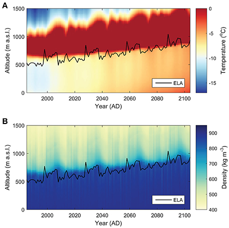
Figure 4. Time-series of annual mean subsurface temperature at 15-m depth (A) and mean density in the first 10 m (B) between 1984 and 2104, plotted as a function of elevation. The black line shows the evolution of the ELA. Years on the x-axis are defined between 1 September (preceding year) and 31 August.

The thermodynamic structure of Svalbard glaciers is strongly influenced by latent heat release after refreezing, which is dominant in the lower accumulation zone where deep percolation and water storage can occur (Van Pelt and Kohler, 2015; Østby et al., in review). The current and projected thermodynamic structure with cold deep subsurface temperatures in the ablation area and temperate conditions in the lower accumulation area is common for Svalbard glaciers (Björnsson et al., 1996; Pettersson, 2004). It is noteworthy that the simulated subsurface temperature development during the reference period (1984–2014) resembles what has recently been observed at a high elevation site (1200 m a.s.l.) on Nordenskiöldbreen in central Spitsbergen. Observed temperatures at 12 m depth in a medium-length borehole in 1998 (Van de Wal et al., 2002) and in a shallow borehole in 2012 (Van Pelt et al., 2014) revealed a warming from cold to temperate conditions, which is in line with the simulated results shown in Figure 4A.

At high elevations in the accumulation zone the percolation depth of melt/rain water is limited and the winter cold wave is sufficiently strong to refreeze all stored water in the course of the winter season. This is not the case in the lower accumulation zone, where water stored deep in the firn (at more than a few meter depth) may survive the winter cooling. At these elevations temperate deep firn conditions remain and in case discharge through crevasses and moulins is low, deep firn water reservoirs (perennial firn aquifers) can potentially develop on top of the impermeable ice. As shown by Kuipers Munneke et al. (2014) the formation of deep perennial temperate firn requires moderate to high melt rates and high accumulation rates. After the discovery of perennial firn aquifers in Greenland (Forster et al., 2013), similar deep firn water reservoirs have recently been detected in ground-penetrating radar data in Svalbard in the accumulation zones on Lomonosovfonna (R. Pettersson, personal communication, 2016) and Holtedahlfonna (Christianson et al., 2015). Without appropriate physics in the model to simulate firn aquifer build-up and dynamics, we limit ourselves to identifying locations of potential firn aquifer development.

The projected subsurface development in Figure 4A reveals substantial warming of deep (ice) temperatures in the ablation area in response to increasing surface temperatures. The elevation band with temperate firn conditions in the lower accumulation zone is found to (1) migrate upwards in response to ELA retreat, and (2) to cover a larger elevation range in a warming climate (Figure 4A). Increased melt rates cause firn degradation and gradual depletion (Figure 4B), causing the firn line to migrate upwards with a delay of typically a few years relative to the rising ELA. The time-delay between ELA rise, firn line retreat and upward extension of the temperate firn zone is an indicator of the sensitivity of firn conditions to changing surface conditions. Widening of the temperate firn zone (Figure 4A) can be explained by an increased significance of rainfall at high elevations, as well as to preferential winter warming, causing a reduction of subsurface cold content at the start of the melt season.

Elevation profiles of mass balance for the periods 1984–2014, 2014–2044, 2044–2074, and 2074–2104 in Figure 5A reveal slightly accelerating upward migration of the ELA. The mean ELA equals 564 m a.s.l. for 1984–2014, 644 m a.s.l. for 2014–2044, 733 m a.s.l. for 2044–2074, and 831 m a.s.l. for 2075–2104. In line with the accelerated ELA rise, the mass balance sensitivity in the ablation area is found to increase in a future climate causing accelerated mass loss toward the end of the simulation period (Figure 5A). Elevation profiles of refreezing (Figure 5B) show values ranging between 0.07 and 0.35 m w.e. a⁻¹ for all periods, with patterns consistently showing a maximum of refreezing in the lower accumulation zone, in line with previous findings for all Svalbard glaciers (Østby et al., in review) and for individual glaciers in central Svalbard (Van Pelt et al., 2012) and western Svalbard (Van Pelt and Kohler, 2015). A similar distribution with a maximum of refreezing in the accumulation zone has also been shown in other regions, such as on the Tibetan Plateau (Fujita et al., 1996). Comparing height-profiles of refreezing between periods reveals an upward shift of the maximum in time in line with the projected firn line retreat. Widening in time of the elevation band with highest refreezing rates is apparent and explains the aforementioned extension of the temperate firn zone (Figure 4A).

FIGURE 5

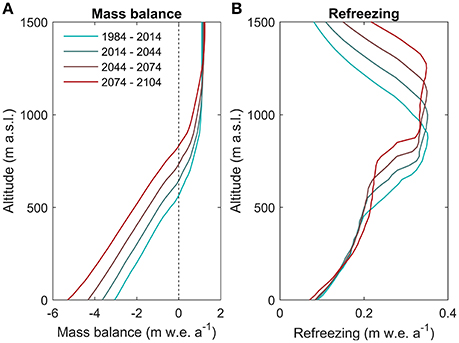
Figure 5. Elevation profiles of the mass balance (A) and refreezing (B) averaged for the periods 1984–2014, 2014–2044, 2044–2074, and 2074–2104. Refreezing in (B) represents total refreezing within the vertical model domain extending down to a depth of 15–20 m.

3.3. Seasonality of Refreezing

Next, we discuss changes in the seasonal pattern of refreezing. The seasonal distribution of refreezing at elevations of 300, 600, and 900 m a.s.l., averaged over three different periods (1984–2014, 2029–2059, and 2074–2104), is shown in Figure 6. During the reference period (1984–2014, Figure 6A), refreezing of melt or rain water is typically most pronounced during the melt season when first melt enters cold seasonal snow or firn, and due to melt-freeze cycles following the daily cycle in temperature and insolation (Colbeck, 1987; Pfeffer and Humphrey, 1998). In the accumulation zone at 900 m a.s.l., a substantial fraction of the total refreezing occurs outside the melt season (Figure 6A) and can be ascribed to refreezing of stored irreducible water, continuing throughout the winter season. During the reference period, small amounts of winter-time refreezing occur at 300 m a.s.l. and can be attributed to rare rainfall events. During the melt season, refreezing at 300 m a.s.l. is mostly concentrated in June-July, when first melt enters the initially cold seasonal snow pack, which disappears in the course of the melt season; higher up, refreezing continues throughout the melt season (Figure 6A).

FIGURE 6

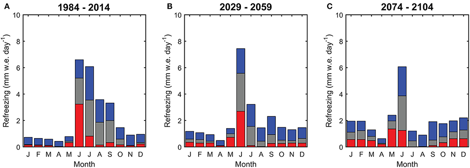
Figure 6. The 30-year mean seasonal distribution of refreezing for the periods 1984-2014 (A), 2029–2059 (B), and 2074–2104 (C) at elevations of 300, 600, and 900 m a.s.l.

In a future climate, refreezing is projected to become less substantial during the melt season and more significant during the winter season at all three elevations (Figures 6B,C). Pronounced winter warming leads to an increased frequency of warm spells with positive temperature excursions, causing increased rainfall occurrence in winter. Latent heat release after refreezing of rain water in winter snow causes snow and firn to warm considerably, which has major implications for the thermodynamic profile and substantially reduces the cold content at the start of the melt season. As a result, refreezing during the melt season will decrease at the expense of winter-time refreezing. An example of this is shown in Figure 3 after a heavy rainfall event in February 2012, 2042, 2072, and 2102.

In contrast to rainfall, surface melting in a warming climate remains very small in winter, mostly due to low or absent solar radiation. For 2074–2104, the ratio of summed melt to summed rainfall between November and March ranges from 3% at 900 m a.s.l. to 20% at 300 m a.s.l., respectively, which confirms that increased future winter-time refreezing is mostly induced by rain events.

3.4. Impact of Refreezing on Subsurface Conditions and Mass Balance

Refreezing of melt and rain water in snow and firn is known to exert a major influence on subsurface temperature and density profiles, and it has been shown to provide a substantial buffer against mass loss of Arctic glaciers (e.g., Wright et al., 2007; Van Angelen et al., 2013). In order to investigate the impact of refreezing on the mass balance, as well as subsurface thermodynamics and stratigraphy, we performed an additional experiment (1984–2104) in which the effects of refreezing are ignored. More specifically, in this experiment we do not allow for any solid mass retention and heat release by refreezing. As a result, all available melt and rain water at the surface will eventually run off; liquid water storage as irreducible water or slush water may still occur and delays runoff. Results of the two runs, averaged over the whole simulation period, are compared in Figure 7.

FIGURE 7

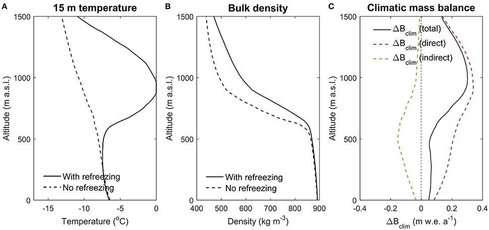
Figure 7. Elevation profiles of subsurface (15-m) temperature (A) and bulk density in the upper 10 m (B), averaged for the period 1984–2104, for a run with and without refreezing. In (C) the net mass balance impact of refreezing is shown and is split into contributions from direct and indirect effects; ΔB_clim (total) is calculated by subtracting climatic mass balance of the no-refreezing run from the refreezing run, ΔB_clim (direct) is the direct effect of refreezing on the climatic mass balance and is equal to total refreezing in the vertical column, and ΔB_clim (indirect) represents the indirect impact of refreezing on the climatic mass balance related to firn heating and densification.

Elevation profiles for the refreezing and no-refreezing runs show a major impact of refreezing on temperatures at 15-m depth, particularly in the lower accumulation zone (Figure 7A). Without refreezing subsurface temperature is only governed by heat conduction and the vertical mass flux and shows a nearly linear decrease with elevation as a result of atmospheric cooling with elevation. Differences of up to 10°C are apparent in the lower accumulation zone. In the ablation area, the impact of refreezing on 15-m subsurface temperature is negligible. Here, heat released by refreezing in seasonal snow is to a large extent removed through melting and discharge of the snow layer.

Without refreezing the vertical density profile in the accumulation zone is determined by gravitational settling and surface accumulation. Solid mass retention by refreezing increases long-term mean bulk density in the upper 10 m by up to 117 kg m⁻³ in the lower accumulation zone (Figure 7B). Averaged over the simulation period and the elevation range 900–1500 m a.s.l., i.e., above the maximum firn line elevation, we find relative contributions to total densification of compaction and refreezing of 64 and 36%, respectively.

Refreezing of percolating or stored water reduces the amount of melt and rain water that runs off, which implies a positive direct impact on the mass balance. However, due to indirect effects after refreezing, as a result of firn heating and densification, the impact of refreezing on the climatic mass balance is not necessarily equal to the amount of refreezing itself. Firstly, heat release during refreezing increases subsurface temperatures, inducing a more positive (or less negative) conductive heat flux at the surface, with the positive flux direction defined toward the surface. A more positive conductive heat flux at the surface may result in higher melt rates as surface temperatures are more readily raised to melting point. Secondly, refreezing adds solid mass to the snow pack and may create ice layers, which, when exposed at the surface, lowers the surface albedo and enhances melt rates. Thirdly, the mass addition by refreezing may prolong the lifetime of seasonal snow and thus reduces the period of bare-ice exposure in summer, thereby reducing surface melt. In order to quantify the net impact of refreezing on the climatic mass balance, we calculate the difference between the climatic mass balance (B_clim) in the refreezing and no-refreezing experiments (ΔB_clim; “refreezing” minus “no-refreezing”; black line in Figure 7C). The total ΔB_clim (black line) is positive at all elevations (Figure 7C), indicating a general positive impact of refreezing on the mass balance. The direct ΔB_clim (red line) refers to the direct mass retaining effect of refreezing, and is equal to the amount of refreezing itself (equivalent to the mean of the four lines in Figure 5B). By differencing the total and direct mass balance effect of refreezing, we estimate the net indirect effect of refreezing (green line in Figure 7C). The net indirect impact of refreezing is the summed effect of the three aforementioned indirect effects; this sensitivity experiment does not allow us to further distinguish individual contributions. The net impact of indirect effects on the mass balance is negative, which indicates that the positive indirect effect (potential prolongation of snow cover) is more than compensated for by negative indirect effects (melt enhancement due to snow pack heating and ice layer formation). A maximum net impact of indirect effects is found in the high ablation area at an approximate elevation of 500 m a.s.l. Averaged over the 0–1500 m a.s.l. elevation range, the mass balance effect of refreezing is 31% smaller than refreezing itself.

3.5. Climate Sensitivity

The above results are sensitive to the chosen future climate scenario, described in Section 2.2. To quantify this sensitivity we performed additional runs for the period 1984–2104 with perturbed precipitation and temperature trends. Sensitivity experiments include runs with zero long-term seasonal trends in temperature (“no ΔT” scenario) and precipitation (“no ΔP” scenario), and runs in which seasonal trends are doubled for temperature (“double ΔT” scenario) and precipitation (“double ΔP” scenario). We additionally perform an experiment in which inhomogeneity in warming of warm and cold spells is ignored (“no spell correction scenario”). For the “no ΔT,” “double ΔT,” “no ΔP” and “double ΔP” scenarios, sensitivity of the mass balance, deep temperature (15-m) and bulk density (0–10 m) is shown in Figure 8. For all experiments sensitivity values, averaged over the elevation range 0–1500 m a.s.l., are presented in Table 1.

FIGURE 8

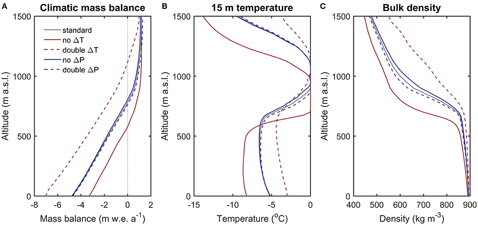
Figure 8. Sensitivity of the 2014–2104 mean climatic mass balance (A), 15-m subsurface temperature (B) and the 0–10 m bulk density (C) for a range of future climate scenarios.

TABLE 1

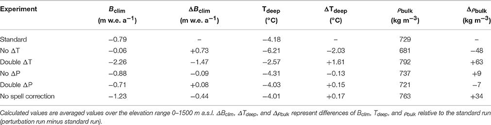
Table 1. Sensitivity of the 2014–2104 mean climatic mass balance (B_clim), 15-m deep temperature (T_deep) and 0–10 m bulk density (ρ_bulk) to different temperature and precipitation scenarios.

Due to relatively weak trends for precipitation in the standard run, the mass balance, deep temperature and bulk density are all found to be much more sensitive to perturbations of the temperature scenario than perturbations of the precipitation scenario (Table 1; Figure 8). Averaged over the 0–1500 m a.s.l. elevation range the mass balance responds about twice as strong to doubling of future seasonal temperature trends than to a no-change scenario, which indicates a strong non-linearity of the mass balance sensitivity to temperature changes (Table 1). The mass balance sensitivity to temperature changes is highest in the ablation zone and decreases with elevation (Figure 8A), in line with previous findings in Van Pelt et al. (2012). In a “double ΔT” scenario a mean future ELA for the period 2014–2104 of 1125 m a.s.l., and 1330 m a.s.l. for the period 2074–2104, would imply that nearly all glaciers in Svalbard would have maximum elevations below the ELA toward the end of the twenty-first century (Nuth et al., 2013). Finally, ignoring inhomogeneity in warming of cold and warm spells (“no spell correction scenario”) has a modest negative impact on the simulated elevation-averaged mass balance (Table 1); in this sensitivity experiment, seasonal warm extremes are amplified leading to higher summer melt rates, thereby enhancing future mass loss.

Deep temperatures and bulk densities in a “double ΔT” scenario, averaged over the period 2014–2104, are strongly influenced by rapid upward migration of the ELA, which effectively smooths out the elevation-dependent variability seen in the “no ΔT” scenario, in which long-term trends in the ELA are absent (Figure 8B). Doubling of temperature trends causes pronounced subsurface warming with respect to the standard run (Table 1), yet cold deep temperature conditions remain in the ablation area even during the last 30 years of the simulation. Based on the above, it seems very unlikely that the general thermodynamic structure with cold deep temperatures in the ablation area and temperate conditions in the lower accumulation zone will change in the near-future. The impact of the “no spell correction scenario” on elevation-averaged deep temperatures is small, while the impact on density is substantial (Table 1). The latter can be ascribed to an increased significance of rainfall and subsequent refreezing in winter due to higher temperatures during warm spells.

As described in Section 2.2.2, we use fixed elevation lapse rates for temperature and precipitation. In practice, temperature and precipitation lapse rates may vary in space and we test the sensitivity of the modeled results to typical lapse rate perturbations representing regional variability across Svalbard. The magnitude of the chosen temperature lapse rate perturbations (±0.0010°C m⁻¹), relative to the standard value of -0.0053°C m⁻¹, reflects variability in reported values across Svalbard, ranging from -0.0040 (Gardner et al., 2009) to -0.0066°C m⁻¹ (Nuth et al., 2012). Sand et al. (2003) reported precipitation lapse rates for Svalbard ranging from 0 to 2.6 mm w.e. a⁻¹ m⁻¹; based on this, we perform sensitivity experiments with the standard value (0.97 mm w.e. a⁻¹ m⁻¹) perturbed by ±1.0 mm w.e. a⁻¹ m⁻¹. Sensitivity results are averaged over the period 2014–2104 for the elevation range 0–1500 m a.s.l., and summarized in Table 2. The mass balance, deep temperature and bulk density are most sensitive to the applied perturbations of the precipitation lapse rate. The impact of temperature lapse rate perturbations is typically about half the impact of the precipitation lapse rate perturbations. Table 2 further reveals that the mass balance is more sensitive to positive temperature and negative precipitation lapse rate changes than to perturbations of opposite sign. Furthermore, the high impact of negatively perturbing the precipitation lapse rate can be ascribed to low precipitation for the whole elevation range in this experiment, which has a severe impact on firn area extent, subsurface temperature and density. Altogether, the above suggests larger regional variability in mass balance and subsurface conditions can be expected from spatial variation of precipitation lapse rates rather than temperature lapse rates.

TABLE 2

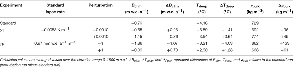
Table 2. Sensitivity of the 2014–2104 mean climatic mass balance (B_clim), 15-m deep temperature (T_deep) and 0–10 m bulk density (ρ_bulk) to different lapse rates for temperature (γ_T) and precipitation (γ_P).

4. Conclusions

Model experiments with a coupled surface energy balance—firn model (EBFM) were done to investigate the climatic mass balance and the changing role of snow and firn conditions in an idealized Svalbard glacier setting. A climate forcing is generated on an elevation-dependent grid for the past, present and future (1984–2104), based on observational data from Svalbard Airport, observation-based elevation lapse rates, and a seasonally dependent projection scenario from an ensemble of future RCM runs. Experiments include a standard run and a set of sensitivity experiments to quantify the impact of refreezing and to assess sensitivity of the results to the chosen climate scenario and elevation lapse rates.

Results illustrate ongoing and future firn degradation and (delayed) firn line retreat in response to an upward ELA migration of 31 m a.s.l. decade⁻¹ between 1984–2104. In a future climate, the elevation band with temperate deep firn in the lower accumulation area, caused by deep percolation, liquid water storage and year-round refreezing, is found to migrate upwards and expand. The cold ablation area warms considerably, yet remains non-temperate toward the end of the twenty-first century. In a future climate, refreezing remains of similar significance, with maximum refreezing rates occurring in the (retreating) lower accumulation zone. In response to pronounced winter warming and an associated increase in winter rainfall, the current prevalence of refreezing during the melt season gradually shifts to the winter season in a future climate. This can be ascribed to more frequent and substantial heat release in the winter snow pack after rainfall events, which in turn reduces the refreezing potential at the start of the melt season.

Comparison of the standard run and a no-refreezing experiment reveals that in a present and future climate the density and thermodynamic structure of Svalbard glaciers are heavily influenced by solid mass retention and heat release after refreezing. By computing the mass balance difference of the refreezing and no-refreezing experiments, we further quantified the mass balance impact of refreezing. The total mass balance effect is found to be positive at all elevations, indicating refreezing acts as a net buffer against mass loss. However, the mass balance effect of refreezing is found to be 31% smaller than mass retention by refreezing itself. This discrepancy is caused by indirect effects after refreezing, related to snow/firn heating, density changes and snow cover changes, which collectively have a negative mass balance impact that partly offsets the mass gain through melt water retention.

Climate sensitivity experiments with perturbed climate scenarios indicate a much higher sensitivity of mass balance, subsurface temperature and bulk density to the prescribed temperature than the precipitation scenario. Experiments with perturbed elevation lapse rates, based on observed regional variability across Svalbard, show a higher sensitivity of the results to precipitation lapse rate changes than to temperature lapse rate perturbations.

Our main aim with this work was to assess the role of snow/firn conditions and refreezing on the mass balance of glaciers in rapidly changing Svalbard climate. For this we chose an idealized elevation-dependent grid, which facilitated the presented analysis with a focus on process-understanding and a discussion of the role of feedbacks. Overall, the results indicate a decisive role for transient snow and firn conditions, and in particular refreezing, on glacier mass loss. This motivates the coupling of surface models to detailed snow models accounting for the subsurface thermodynamic, density and water content evolution in large-scale applications.

Author Contributions

WvP performed the model experiments and wrote the manuscript. WvP, VP, and CR discussed the approach and model outcome. VP and CR provided thorough comments and feedback on the manuscript that helped to improve the manuscript quality.

Conflict of Interest Statement

The authors declare that the research was conducted in the absence of any commercial or financial relationships that could be construed as a potential conflict of interest.

Acknowledgments

Meteorological data from the Svalbard Airport weather station were downloaded from the eKlima portal (www.eklima.no), provided by the Norwegian Meteorological Institute. We thank colleagues at Uppsala University, and in particular S. Marchenko, for discussion, comments and suggestions which have helped to improve the manuscript. Finally, we thank the reviewers and editor for their insightful feedback that has helped to improve the manuscript.

References

ACIA (2005). Arctic Climate Impact Assessment - Scientific Report. New York, NY: Cambridge University Press.

Baumberger, A. (2007). Massebalans på Kronebreen/Holtedahlfonna, Svalbard - kontrollerende faktorer. Master thesis, University of Oslo.

Bengtsson, L., Hodges, K. I., Koumoutsaris, S., Zahn, M., and Keenlyside, N. (2011). The changing atmospheric water cycle in Polar Regions in a warmer climate. Tellus A 63A, 907–920. doi: 10.1111/j.1600-0870.2011.00534.x

CrossRef Full Text | Google Scholar

Bintanja, R., and Selten, F. M. (2014). Future increases in Arctic precipitation linked to local evaporation and sea-ice retreat. Nature 509, 479–482. doi: 10.1038/nature13259

PubMed Abstract | CrossRef Full Text | Google Scholar

Bintanja, R., and van der Linden, E. C. (2013). The changing seasonal climate in the Arctic. Sci. Rep. 3, 1–8. doi: 10.1038/srep01556

PubMed Abstract | CrossRef Full Text | Google Scholar

Björnsson, H., Gjessing, Y., Hamran, S.-E., Hagen, J. O., Liestøl, O., Palsson, F., et al. (1996). The thermal regime of sub-polar glaciers mapped by multi-frequency radio-echo sounding. J. Glaciol. 42, 23–32.

Google Scholar

Blaszczyk, M., Jania, J. A., and Hagen, J. O. (2009). Tidewater glaciers of Svalbard: recent changes and estimates of calving fluxes. Polish Polar Res. 30, 85–142.

Google Scholar

Christianson, K., Kohler, J., Alley, R. B., Nuth, C., and Van Pelt, W. J. (2015). Dynamic perennial firn aquifer on an Arctic glacier. Geophys. Res. Lett. 42, 1418–1426. doi: 10.1002/2014GL062806

CrossRef Full Text | Google Scholar

Cogley, J. G., Hock, R., Rasmussen, L. A., Arendt, A. A., Bauder, A., Braithwaite, R. J., et al. (2011). Glossary of Glacier Mass Balance and Related Terms. Technical report, IHP-VII Technical Documents in Hydrology No. 86, IACS Contribution No. 2, UNESCO-IHP, Paris.

Colbeck, S. C. (1987). “A review of the metamorphism and classification of seasonal snow cover crystals,” in Avalanche Formation, Movement and Effects, Proceedings of the Davos Symposium, September 1986.

Google Scholar

Day, J. J., Bamber, J. L., Valdes, P. J., and Kohler, J. (2012). The impact of a seasonally ice free Arctic Ocean on the temperature, precipitation and surface mass balance of Svalbard. Cryosphere 6, 35–50. doi: 10.5194/tc-6-35-2012

CrossRef Full Text | Google Scholar

Divine, D. V., and Dick, C. (2006). Historical variability of sea ice edge position in the Nordic Seas. J. Geophys. Res. 111:C01001. doi: 10.1029/2004JC002851

CrossRef Full Text | Google Scholar

Førland, E. J., Benestad, R., Hanssen-Bauer, I., Haugen, J. E., and Skaugen, T. E. (2011). Temperature and precipitation development at svalbard 1900–2100. Adv. Meteorol. 2011, 1–14. doi: 10.1155/2011/893790

CrossRef Full Text | Google Scholar

Førland, E. J., and Hanssen-Bauer, I. (2000). Increased precipitation in the Norwegian Arctic: true or false? Clim. Change 46, 485–509. doi: 10.1023/A:1005613304674

PubMed Abstract | CrossRef Full Text | Google Scholar

Forster, R. R., Box, J. E., Van den Broeke, M. R., Miège, C., Burgess, E. W., Van Angelen, J. H., et al. (2013). Extensive liquid meltwater storage in firn within the Greenland ice sheet. Nat. Geosci. 7, 95–98. doi: 10.1038/ngeo2043

CrossRef Full Text | Google Scholar

Fujita, K., Seko, K., Ageta, Y., Jianchen, P., and Tandong, Y. (1996). Superimposed ice in glacier mass balance on the Tibetan Plateau. J. Glaciol. 42, 454–460.

Google Scholar

Gardner, A. S., Sharp, M. J., Koerner, R. M., Labine, C., Boon, S., Marshall, S. J., et al. (2009). Near-surface temperature lapse rates over Arctic glaciers and their implications for temperature downscaling. J. Climate 22, 4281–4298. doi: 10.1175/2009JCLI2845.1

CrossRef Full Text | Google Scholar

Greuell, W., and Konzelmann, T. (1994). Numerical modelling of the energy balance and the englacial temperature of the Greenland Ice Sheet. Calculations for the ETH-Camp location (West Greenland, 1155 m a.s.l.). Glob. Planet. Change 9, 91–114. doi: 10.1016/0921-8181(94)90010-8

CrossRef Full Text | Google Scholar

Hagen, J. O., Kohler, J., Melvold, K., and Winther, J.-G. (2003). Glaciers in Svalbard: mass balance, runoff and freshwater flux. Polar Res. 22, 145–159. doi: 10.1111/j.1751-8369.2003.tb00104.x

CrossRef Full Text | Google Scholar

Hanssen-Bauer, I., and Førland, E. (1998). Long-term trends in precipitation and temperature in the Norwegian Arctic: can they be explained by changes in atmospheric circulation patterns? Clim. Res. 10, 143–153. doi: 10.3354/cr010143

CrossRef Full Text | Google Scholar

IPCC (2013). Climate Change 2013: The Physical Science Basis. Contribution of Working Group I to the Fifth Assessment Report of the Intergovernmental Panel on Climate Change [Stocker, T.F., D. Qin, G. - K. Plattner, M. Tignor, S.K. Allen, J. Bosc hung, A. Nauels, Y. X. Cambridge; New York: Cambridge University Press.

James, T. D., Murray, T., Barrand, N. E., Sykes, H. J., Fox, A. J., and King, M. A. (2012). Observations of enhanced thinning in the upper reaches of Svalbard glaciers. Cryosphere 6, 1369–1381. doi: 10.5194/tc-6-1369-2012

CrossRef Full Text | Google Scholar

Jania, J., Mochnacki, D., and Gadek, B. (1996). The thermal structure of Hansbreen, a tidewater glacier in southern Spitsbergen, Svalbard. Polar Res. 15, 53–66. doi: 10.1111/j.1751-8369.1996.tb00458.x

CrossRef Full Text | Google Scholar

Klok, E. L., and Oerlemans, J. (2002). Model study of the spatial distribution of the energy and mass balance of Morteratschgletscher, Switzerland. J. Glaciol. 48, 505–518. doi: 10.3189/172756502781831133

CrossRef Full Text | Google Scholar

Konzelmann, T., van de Wal, R., Greuell, W., Bintanja, R., Henneken, E., and Abeouchi, A. (1994). Parameterization of global and longwave incoming radiation for the Greenland Ice Sheet. Glob. Planet. Change 9, 143–164. doi: 10.1016/0921-8181(94)90013-2

CrossRef Full Text | Google Scholar

Kuipers Munneke, P., M. Ligtenberg, S. R., Van den Broeke, M. R., Van Angelen, J. H., and Forster, R. R. (2014). Explaining the presence of perennial liquid water bodies in the firn of the Greenland Ice Sheet. Geophys. Res. Lett. 41, 476–483. doi: 10.1002/2013GL058389

CrossRef Full Text | Google Scholar

Lang, C., Fettweis, X., and Erpicum, M. (2015). Stable climate and surface mass balance in Svalbard over 1979-2013 despite the Arctic warming. Cryosphere 9, 83–101. doi: 10.5194/tc-9-83-2015

CrossRef Full Text | Google Scholar

Ligtenberg, S. R. M., Helsen, M. M., and Van Den Broeke, M. R. (2011). An improved semi-empirical model for the densification of Antarctic firn. Cryosphere 5, 809–819. doi: 10.5194/tc-5-809-2011

CrossRef Full Text | Google Scholar

Machguth, H., MacFerrin, M., Van As, D., Box, J. E., Charalampidis, C., Colgan, W., et al. (2016). Greenland meltwater storage in firn limited by near-surface ice formation. Nat. Clim. Change 6, 390–393. doi: 10.1038/nclimate2899

CrossRef Full Text | Google Scholar

Min, S.-K., Zhang, X., and Zwiers, F. (2008). Human-induced Arctic moistening. Science (New York, N.Y.) 320, 518–520. doi: 10.1126/science.1153468

PubMed Abstract | CrossRef Full Text | Google Scholar

Min, S.-K., Zhang, X., Zwiers, F. W., and Hegerl, G. C. (2011). Human contribution to more-intense precipitation extremes. Nature 470, 378–381. doi: 10.1038/nature09763

PubMed Abstract | CrossRef Full Text | Google Scholar

Möller, M., Obleitner, F., Reijmer, C. H., Pohjola, V. A., Głowacki, P., and Kohler, J. (2016). Adjustment of regional climate model output for modeling the climatic mass balance of all glaciers on Svalbard. J. Geophys. Res. Atmospheres. 121, 5411–5429. doi: 10.1002/2015JD024380

PubMed Abstract | CrossRef Full Text | Google Scholar

Nordli, Ø., Przybylak, R., Ogilvie, A. E., and Isaksen, K. (2014). Long-term temperature trends and variability on Spitsbergen: the extended Svalbard Airport temperature series, 1898–2012. Polar Res. 33:21349. doi: 10.3402/polar.v33.21349

CrossRef Full Text | Google Scholar

Nuth, C., Kohler, J., König, M., Von Deschwanden, A., Hagen, J. O., Kääb, A., et al. (2013). Decadal changes from a multi-temporal glacier inventory of Svalbard. Cryosphere 7, 1603–1621. doi: 10.5194/tc-7-1603-2013

CrossRef Full Text | Google Scholar

Nuth, C., Schuler, T. V., Kohler, J., Altena, B., and Hagen, J. O. (2012). Estimating the long-term calving flux of Kronebreen, Svalbard, from geodetic elevation changes and mass-balance modelling. J. Glaciol. 58, 119–133. doi: 10.3189/2012JoG11J036

CrossRef Full Text | Google Scholar

Oerlemans, J., and Grisogono, B. (2002). Glacier winds and parameterization of the related surface heat fluxes. Tellus 54A, 440–452. doi: 10.1034/j.1600-0870.2002.201398.x

CrossRef Full Text | Google Scholar

Oerlemans, J., and Knap, W. H. (1998). A 1 year record of global radiation and albedo in the ablation zone of Morteratschgletscher, Switzerland. J. Glaciol. 44, 231–238.

Google Scholar

Pettersson, R. (2004). Dynamics of the Cold Surface Layer of Polythermal storglaciären, Sweden. Ph.D. thesis, Stockholm University, Department of Physical Geography and Quaternary Geology. Stockholm University Dissertation Series.

Pfeffer, W. T., and Humphrey, N. (1998). Formation of ice layers by infiltration and refreezing of meltwater. Ann. Glaciol. 26, 83–91.

Google Scholar

Pfeffer, W. T., Meier, M. F., and Illangasekare, T. H. (1991). Retention of Greenland runoff by refreezing: implications for projected future sea level change. J. Geophys. Res. 96, 117–122. doi: 10.1029/91JC02502

CrossRef Full Text | Google Scholar

Reijmer, C. H., and Hock, R. (2008). Internal accumulation on Storglaciären, Sweden, in a multi-layer snow model coupled to a distributed energy- and mass-balance model. J. Glaciol. 54, 61–72. doi: 10.3189/002214308784409161

CrossRef Full Text | Google Scholar

Reijmer, C. H., Van Den Broeke, M. R., Fettweis, X., Ettema, J., and Stap, L. B. (2012). Refreezing on the Greenland ice sheet: a comparison of parameterizations. Cryosphere 6, 743–762. doi: 10.5194/tc-6-743-2012

CrossRef Full Text | Google Scholar

Sand, K., Winther, J.-G., Marechal, D., Bruland, O., and Melvold, K. (2003). Regional variations of snow accumulation on spitsbergen, svalbard, 1997-99. Nordic Hydrol. 34, 17–32.

Google Scholar

Serreze, M. C., Crawford, A. D., and Barrett, A. P. (2015). Extreme daily precipitation events at Spitsbergen, an Arctic Island. Int. J. Climatol. 35, 4574–4588. doi: 10.1002/joc.4308

CrossRef Full Text | Google Scholar

Serreze, M. C., and Francis, J. A. (2006). The Arctic amplification debate. Clim. Change 76, 241–264. doi: 10.1007/s10584-005-9017-y

CrossRef Full Text | Google Scholar

Van Angelen, J. H., Lenaerts, J. T. M., Van den Broeke, M. R., Fettweis, X., and Van Meijgaard, E. (2013). Rapid loss of firn pore space accelerates 21st century Greenland mass loss. Geophys. Res. Lett. 40, 2109–2113. doi: 10.1002/grl.50490

CrossRef Full Text | Google Scholar

Van de Wal, R. S. W., Mulvaney, R., Isaksson, E., Moore, J. C., Pinglot, J. F., Pohjola, V. A., et al. (2002). Reconstruction of the historical temperature trend from measurements in a medium-length borehole on the Lomonosovfonna plateau, Svalbard. Ann. Glaciol. 35, 371–378. doi: 10.3189/172756402781816979

CrossRef Full Text | Google Scholar

Van Pelt, W. J. J., and Kohler, J. (2015). Modelling the long-term mass balance and firn evolution of glaciers around Kongsfjorden, Svalbard. J. Glaciol. 61, 731–744. doi: 10.3189/2015JoG14J223

CrossRef Full Text | Google Scholar

Van Pelt, W. J. J., Oerlemans, J., Reijmer, C. H., Pettersson, R., Pohjola, V. A., Isaksson, E., et al. (2013). An iterative inverse method to estimate basal topography and initialize ice flow models. Cryosphere 7, 987–1006. doi: 10.5194/tc-7-987-2013

CrossRef Full Text | Google Scholar

Van Pelt, W. J. J., Oerlemans, J., Reijmer, C. H., Pohjola, V. A., Pettersson, R., and Van Angelen, J. H. (2012). Simulating melt, runoff and refreezing on Nordenskiöldbreen, Svalbard, using a coupled snow and energy balance model. Cryosphere 6, 641–659. doi: 10.5194/tc-6-641-2012

CrossRef Full Text | Google Scholar

Van Pelt, W. J. J., Pettersson, R., Pohjola, V. A., Marchenko, S., Claremar, B., and Oerlemans, J. (2014). Inverse estimation of snow accumulation along a radar transect on Nordenskiöldbreen, Svalbard. J. Geophys. Res. Earth Surf. 119, 816–835. doi: 10.1002/2013JF003040

CrossRef Full Text | Google Scholar

Vega, C. P., Pohjola, V. A., Beaudon, E., Claremar, B., Van Pelt, W. J. J., Pettersson, R., et al. (2016). A synthetic ice core approach to estimate ion relocation in an ice field site experiencing periodical melt: a case study on Lomonosovfonna, Svalbard. Cryosphere 10, 961–976. doi: 10.5194/tc-10-

CrossRef Full Text | Google Scholar

Winther, J.-G., Bruland, O., Sand, K., Gerland, S., Marechal, D., Ivanov, B., et al. (2003). Snow research in Svalbard – an overview. Polar Res. 22, 125–144. doi: 10.1111/j.1751-8369.2003.tb00103.x

CrossRef Full Text | Google Scholar

Wright, A. P., Wadham, J. L., Siegert, M. J., Luckman, A., Kohler, J., and Nuttall, A.-M. (2007). Modeling the refreezing of meltwater as superimposed ice on a high Arctic glacier: a comparison of approaches. J. Geophys. Res. 112:F04016. doi: 10.1029/2007jf000818

CrossRef Full Text | Google Scholar

Zhang, X., He, J., Zhang, J., Polyakov, I., Gerdes, R., Inoue, J., et al. (2012). Enhanced poleward moisture transport and amplified northern high-latitude wetting trend. Nat. Clim. Change 3, 47–51. doi: 10.1038/nclimate1631

CrossRef Full Text | Google Scholar