Determining the Stress Field in Active Volcanoes Using Focal Mechanisms

Introduction

Theoretical Background to Stress Field Inversion

In last decades focal mechanisms have shown to be very useful to infer about the stress field within the Earth. Being seismicity a common feature of both quiescent and erupting volcanoes, the study of volcano-tectonic earthquakes is an effective tool to retrieve spatial and temporal patterns in the pre-, syn-, and inter-eruptive stress fields. Stress changes associated with magma migration and more in general with the dynamics of magma chambers and hydrothermal systems are causally linked to these earthquakes. Hence retrieving the stress field pattern in volcanoes has important implications in studying their dynamics and the interaction with the regional tectonic stress field (Umakoshi et al., 2001; Pedersen and Sigmundsson, 2004; Segall, 2013; Cannavò et al., 2014; D'Auria et al., 2014a,b).

Rocks in the Earth lithosphere possess a specific state of stress strictly related to the tectonic setting of the region. The state of stress at any given point can be represented geometrically as a Stress Ellipsoid, a tri-axial solid built with the Principal Stress Components (PSC) σ₁ > σ₂ > σ₃ as main axes. The shape of this ellipsoid can be expressed using the Bishop's ratio Φ_B = (σ₂ − σ₃) / (σ₁ − σ₃) (Bishop, 1966). It expresses the relationship between the intermediate and maximum PSC respect to the minimum one and can assume values varying from 0 to 1. In a general tri-axial state of stress σ₁ > σ₂ > σ₃ ≠ 0, and the Φ_B ≈ 0.5. A slip event along a fault surface occurs when the accumulated energy exceeds the internal strength of the rock (Reid, 1910). The rupture starts at the hypocenter and then propagates along the whole fault plane. Analysis of seismograms allows the retrieving of information about the seismogenic structure responsible for an event. Byerly (1928) proposed a method that allows the reconstruction of the Fault Plane Solution (FPS) of an earthquake, which is a stereographic projection representing the geometry of a seismogenic structure. It can be easily explained picturing a focal sphere ideally located around the earthquake hypocenter. The focal sphere can be separated into four dihedra, two contractional, and two dilatational, delimited by two planes known as Nodal Planes (the main and the auxiliary planes). The main nodal plane represents the actual fault, with the slip occurring during the earthquake being along the direction orthogonal to the auxiliary plane (Figure 1). Therefore the geometry of the FPS is tightly linked to the fault kinematics. At the center of the contractional dihedra is located the P-axis (compressive) while the center of extensional dihedra (dilatational) hosts the T-axis. The neutral B-axis corresponds to the intersection of nodal planes (Figure 1). P, T, B axes are mutually normal. The relationship between P and T axes of a FPS and the actual σ₁ and σ₃ stress directions is not straightforward. The aim of stress inversion techniques is precisely to determine it. A FPS can be reconstructed a posteriori, starting from the analysis of the first arrival of P-waves at an adequate number of seismographs arranged around the hypocenter. Using the equal-area stereographic projection technique (lower hemisphere), each station can be plotted using the angular coordinates of the direct seismic ray leaving the hypocenter. Stations falling in a contractional quadrant will record a downward first P-wave arrival (void circle of Figure 1A). Conversely, stations falling in a dilatational quadrant will register an upward first P-wave arrival (solid circle of Figure 1A). Plotting this information on an equal-area stereographic projection net it is possible to find a couple of nodal planes that is able to divide up the plot into four quadrants, corresponding to the four dihedra of the focal sphere (Figure 1). Nowadays, these procedures are implemented in a wide range of algorithms performing the determination of the FPS automatically. One of the most commonly used algorithms is FPFIT (Reasenberg and Oppenheimer, 1985). It is a suite of Fortran codes for calculating and displaying earthquake fault-plane solutions. FPFIT finds the double-couple fault plane solution (source model) that best fits a given set of observed first motion polarities for an earthquake.

FIGURE 1

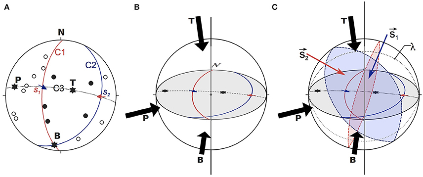
Figure 1. The Byerly's Fault Plane Solution. (A) A FPS is a stereographic projection representing the double-couple model of the seismogenic source; equal-area stereographic projection technique (lower hemisphere), void circles are P-wave downward first arrivals, solid circles are P-wave upward first arrivals, C₁ and C₂ are nodal planes with associated slip vectors s₁ (pole to C₂) and s₂ (pole to C₁), P- (compressive) T- (tensional) and B-axes (neutral) are also plotted; (B) Three-dimensional view of a Focal Sphere, the FPS of (A) represents the stereographic projection (on the equatorial plane) of the geometrical elements intersecting the lower hemisphere. (C) 3-D perspective of the FPS (see text for details).

Starting from observed fault kinematics or focal mechanisms, various stress inversion procedures can be implemented. These procedures allow the reconstruction of the reduced stress field that carries information about the stress orientation and the ratios between principal stresses. Inversion of focal mechanism datasets became a common task in studies aimed at constrain seismotectonic stress field in active tectonic areas (Carey-Gailhardis and Mercier, 1992; Gillard and Wyss, 1995; Hardebeck and Hauksson, 2001; Massa, 2003; Angelier and Baruah, 2009; De Matteis et al., 2012) and more recently also in volcanic environments (Wyss et al., 1992; Cocina et al., 1997; D'Auria et al., 2014a,b; Plateaux et al., 2014). A wide range of graphical and analytical methods were proposed by authors in last decades (e.g., Angelier and Mechler, 1977; Gephart and Forsyth, 1984; Carey-Gailhardis and Mercier, 1987; Lisle, 1987, 1988; Michael, 1987; Angelier, 1990, 2002; Rivera and Cisternas, 1990; D'Auria and Massa, 2015). Stress inversion procedures are based on the Wallace-Bott hypothesis: shear traction acting on a fault plane (irrespective of newly formed structure or a reactivated preexisting one) causes a slip event in the direction and sense of the shear traction itself (Wallace, 1951; Bott, 1959; Angelier and Mechler, 1977; Yamaji, 2007). Analytical techniques of stress inversion are based on the systematic comparison of the actual slip vector with respect to the theoretical (modeled) maximum shear stress acting on the same surface in response to the active stress field (Figure 2). Graphical approaches are based on the definition of a probability function (or an equivalent formulation) on the whole focal sphere. They allow the determination of a range of possible attitudes for principal stress axes using hand stereo-plot. Right Dihedra Method (RDM) represents the simplest of graphical stress inversions (Angelier and Mechler, 1977). It basically consists of averaging the focal spheres of a focal mechanisms dataset. In the late 80's, RDM was improved adding an additional geometrical constrain and was re-proposed as Right Trihedra Method (Lisle, 1987, 1988). Both RDM and RTM are able to manage both planes of focal mechanism regardless the pre-selection of the actual fault plane. D'Auria and Massa (2015) proposed a novel Bayesian approach for the determination of the stress field from focal mechanism datasets (BRTM). This method can be regarded as a re-visitation of the RTM in a sound probabilistic framework. It provides a probability function over the focal sphere for both σ₁ and σ₃ principal stress directions (Figure 3). BRTM algorithm has shown to be robust and efficiently enough to manage all kind of kinematics and nodal plane attitudes. A comparison of the BRTM performances to respect a classical Direct Inversion Method (Angelier, 1990, 2002) and the Multiple Inverse Method (Yamaji, 2000), confirms that BRTM is able to successfully manage both homogeneous and heterogeneous datasets (see Figure 2 in D'Auria and Massa, 2015). Furthermore BRTM allows both a reliable determination of the principal stress axes attitude and a quantitative estimation of the corresponding confidence regions (D'Auria and Massa, 2015). Finally, to give a complete and accurate inversion the corresponding Bishop's ratio Φ_B can be determined, exploiting the BRTM results, following the approach proposed by Angelier (1990; Figure 3). In case of heterogeneous datasets result of stress field inversion could be misleading. The problem can be approached using different un-supervisioned techniques (e.g., Angelier and Manoussis, 1980; Yamaji, 2000). Among those, the Multiple Inverse Method (Yamaji, 2000), makes use of a resampling technique of the analyzed dataset, through the construction of many data subsets, inverted separately using an analytical approach (Otsubo et al., 2008). Results can be plotted on a stereographic projection to outline graphically different clusters of stress tensors, corresponding to the different components of the stress field acting in the lithospheric volume associated to the dataset. The major drawback of this technique is the difficulty in attributing to the retrieved stress field components a proper spatio-temporal collocation. Therefore heterogeneous datasets can be approached, more properly, taking into account spatial and possibly temporal variations of the stress pattern (Wyss et al., 1992; Hardebeck and Michael, 2006; D'Auria et al., 2014b). In other words, these methods take into account the spatio-temporal distribution of the data, providing as results not a single stress tensor, but a spatially (and possibly temporally) variable stress field. Applying the BRTM to subsets of FPS corresponding to a given sub-volume of the area under investigation allows retrieving the spatial pattern of the stress field. This is an essential approach in the analysis of seismological dataset of volcanic districts. In the next section we show the application of stress inversion procedures to three different volcanic areas. Analyses were carried out on datasets available from previous studies. For Mt.Somma-Vesuvius and Campi Flegrei we used data from D'Auria et al. (2014a,b). For the Long Valley Caldera, data are freely accessible to users via the Internet (NCEDC, 2014). We preferred to invert published datasets to novel ones as this allows a more efficient comparison of obtained results got with different processing approaches.

FIGURE 2

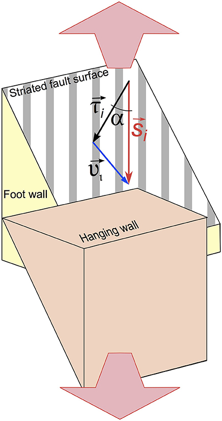
Figure 2. Misfit criteria adopted in stress inversion procedures. α angle formed between the actual slip vector (s_i) and the theoretical shear stress (τ_i) acting on each fault of the analyzed dataset (Carey and Brunier, 1974; Angelier, 1990); υ_i, the vector difference between s_i and τ_i (Angelier, 1990).

FIGURE 3

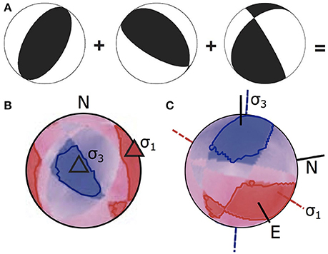
Figure 3. Results of the BRTM applied to a synthetic dataset (A) made up of three FPSs (black = dilatational dihedra); (B) 2-D plot on a Lambert equiareal, lower-hemisphere projection; (C) tridimensional view of the BRTM results over the focal sphere (After: D'Auria and Massa, 2015, modified).

This study aims at highlighting the key role played by stress inversion procedures in the analysis of the volcano dynamics. In detail, we show the methodological potential offered by the BRTM here tested on seismological datasets collected at three different volcanoes.

Case Studies

In order to show the capability of the stress inversion procedures on volcanoes, we applied the BRTM to determine the spatial variations of the stress field in three different volcano-tectonic environments: the Mt. Somma-Vesuvius Volcano (Southern Italy; Figure 4), the Campi Flegrei Caldera (Southern Italy; Figure 4) and the Long Valley Caldera (California-Sierra Nevada border, USA; Figure 9). In the following we report a synthesis of the key results, focusing on the relationship between the local active stress fields and the background regional ones.

FIGURE 4

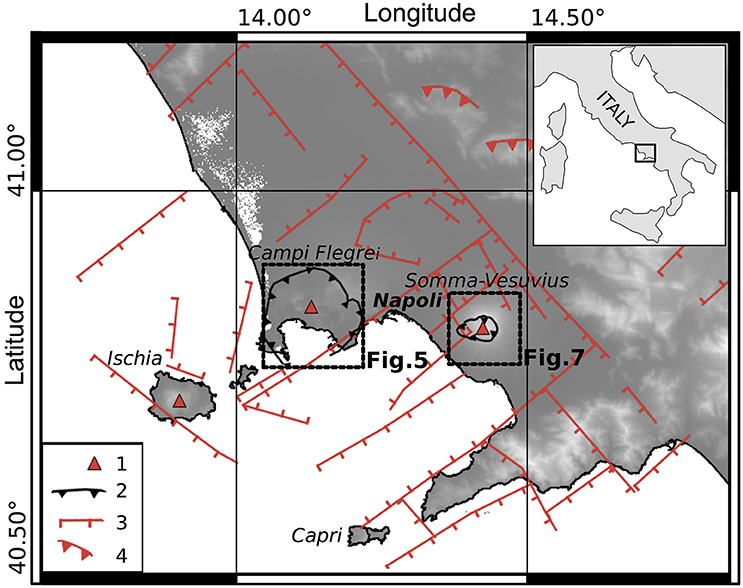
Figure 4. Tectonic setting of the Campi Flegrei-Vesuvius area. (1) Main volcanoes; (2) Campi Flegrei (Campanian Ignimbrite) and Mt. Somma caldera rims; (3) main Plio-Quaternary faults; (4) thrust faults. Dashed squares identify the location of Figures 5, 7. Data from: Ippolito et al., 1973; Di Vito et al., 1999; Lavecchia et al., 2003; Acocella and Funiciello, 2006; Milia et al., 2013; Vitale and Isaia, 2013; D'Auria et al., 2014a,b, and referencer therein.

Mt. Somma-Vesuvius

The Somma-Vesuvius (Figures 4, 5) is the youngest volcano of the Neapolitan district, it is characterized both by explosive and effusive activity (Santacroce, 1987). Its oldest products are dated 0.369 ± 0.028 Ma (⁴⁰Ar/³⁹Ar age from Brocchini et al., 2001). The last eruption of Vesuvius occurred in 1944 and after this event it has become quiescent, showing only fumarolic activity and low seismicity (M ≤ 3.6). Since 1964 to nowadays the seismicity started to increase in the occurrence and in the magnitude (Giudicepietro et al., 2010), with four episodes (1978–1980, 1989–1990, 1995–1996, 1999–2000) of strong increased strain release rate, occurrence and magnitude rate (D'Auria et al., 2013). The Mesozoic basement of the volcano is displaced by both SW- and NW-dipping normal fault systems and secondarily by NE-SW and E-W faults (Bianco et al., 1998; Ventura and Vilardo, 1999; Zollo et al., 2002; Acocella and Funiciello, 2006; Figure 4). Mesoscale faults and eruptive fractures striking NW-SE, NE-SW and ENE-WSW affect volcanic units outside the Somma caldera (Rosi et al., 1987; Andronico et al., 1995; Ventura and Vilardo, 1999; D'Auria et al., 2014a, Figure 1 for a review). Seismicity at Mt. Somma-Vesuvius shows the presence of two different seismogenic volumes: a top volume (above sea level) and a bottom one (1–5 km depth). These two volumes appear to be separated by a volume with a markedly reduced seismic strain release, possibly corresponding to a ductile sedimentary layer buried at about 1000 m b.s.l. (Bernasconi et al., 1981; Borgia et al., 2005; D'Auria et al., 2014a).

FIGURE 5

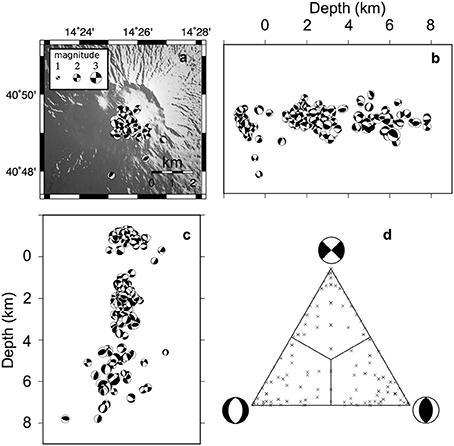
Figure 5. Mt. Somma-Vesuvius. Focal mechanisms dataset plotted on a shaded map (A), on a N-S (B), and an E-W (C) cross sections. (D) The distribution of focal mechanisms on a triangular Frohlich diagram (Frohlich, 1992). The dataset consists of 197 FPSs of earthquakes recorded from 1999 to 2012 with 0 < M < 3.6.

At Mt. Somma-Vesuvius we analyzed a dataset consisting of 197 FPSs of earthquakes recorded from 1999 to 2012 with 0 < M < 3.6 (D'Auria et al., 2014a). All the events were relocated by D'Auria et al. (2014a) using a nonlinear probabilistic approach in a 3-D velocity model (Lomax et al., 2001; D'Auria et al., 2008). FPSs were computed using P wave polarities (Reasenberg and Oppenheimer, 1985). Only events with at least six first motion observations were used to derive FPSs (Figure 5). Kinematics of the analyzed FPSs are quite equally represented in the three extreme categories, dip-slip normal, dip-slip reverse and strike-slip (Figure 5D). The stress field has been computed on a regular three-dimensional grid of 1-km spacing. For each grid node all the FPSs within a radius of 1-km have been considered for the inversion. The stress field has been computed only at volumes containing at least five FPSs. A synthesis of BRTM results is reported in Figure 6. For the top-volume (slice for depth −1 km, corresponding to the portion of the edifice lying above the sea level) the retrieved σ₁ is sub-horizontal overall trending NW-SE, corresponding to a sub-vertical σ₃ and the related Φ_B is <0.5. Results for the bottom volume are summarized for depths of 1, 3, and 5 km. At 1 km depth slice σ₁ moderately plunges toward ENE and corresponds to a sub-horizontal σ₃ trending NNW-SSE. In this case 0.3 < Φ_B < 0.5. At 3 km depth slice the attitude of the σ₁ is highly variable overall plunging toward NNW. It corresponds to a sub-horizontal σ₃ trending E-W in the axial sector, SW-NE and NW-SE at the most external volumes with a Bishop's ratio 0.4 < Φ_B < 0.5. At the deepest depth slice (5 km), σ₁ is sub-horizontal trending NNE-SSW to NW-SE, corresponding to moderately to high plunging σ₃trending ENE-WSW, the Φ_B is high variable experiencing values from 0.2 to 1 (Figure 6). The marked differences in the stress field pattern retrieved within the two seismogenic volumes (Figure 6, slice -1 vs. slices 1-3-5) can be addressed to the effect of the aforementioned decoupling ductile layer. The faulting style active in the top-volume is compatible with a spreading process involving the exposed Somma-Vesuvius edifice, as proposed by various previous studies (see references in D'Auria et al., 2014a). The strain field resulting from the subsidence of the Vesuvius and the asymmetric spreading of the southern portion of the Somma edifice creates an overall NS compression (see Figure 17 in D'Auria et al., 2014a). This ongoing process is also the source of the persistent seismicity located within the top-volume (Borgia et al., 2005; D'Auria et al., 2013, 2014a; Figures 5, 6). Additionally, the low Φ_B values associated to stress inversion in the top volume confirm that the retrieved fields are strongly driven by the σ₁. According to previous studies, the bottom-volume seems to be deeply related to a regional background stress field slightly perturbed by local heterogeneities in the volcanic structure and by the complex topography of the volcano. The intermittent behavior of the seismic activity in the deepest volume is probably due to a relation with the dynamics of the hydrothermal system: the pore pressure within the hydrothermal system can be perturbed by episodes of fluid injection that essentially influence the stress field pattern in the bottom-volume (Figures 5, 6; Chiodini et al., 2001; D'Auria et al., 2014a). The Φ_B values associated to stress inversion in the bottom volume show that for the 1- and 3-km depth-slices the three principal stresses are well defined (overall, 0.3 < Φ_B < 0.5). A quite different result was obtained for the deepest depth-slice, the 5-km one: here Φ_B values show an high variability with values ranging from 0.5 to 1 and a σ₃ overall trending NE-SW. This last result appears in accordance with the local minimum horizontal principal stress component (S_h) measured within the Trecase 1 well (located at the SE slope of the Mt. Somma-Vesuvius) as borehole breakout, showing an elongation in ENE-WSW direction (Montone et al., 2012).

FIGURE 6

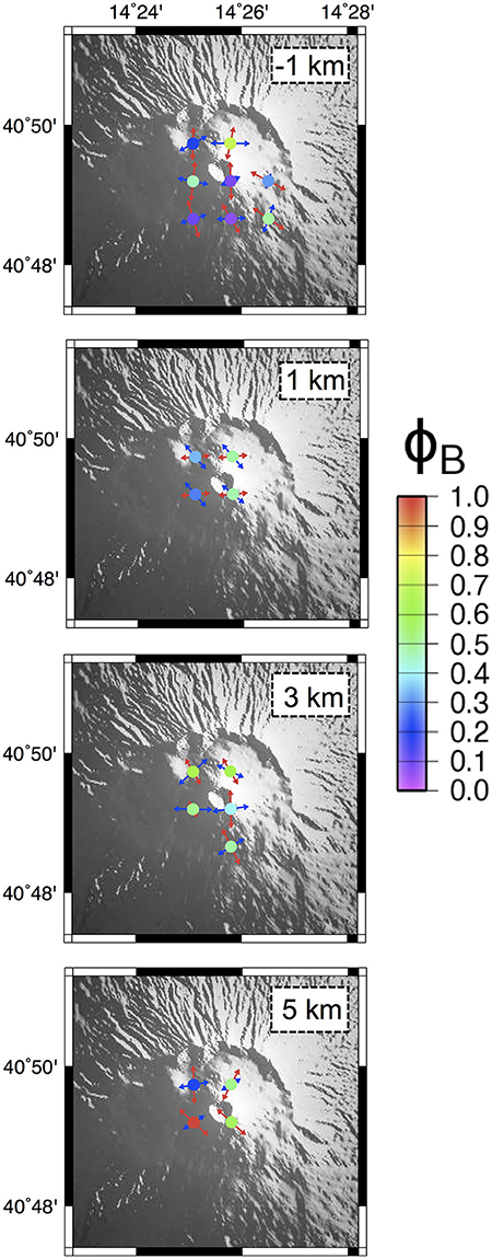
Figure 6. Mt. Somma-Vesuvius. Stress field tensors retrieved from focal mechanisms data using the BRTM. Slices at −1, 1, 3, and 5 km-depth. Stress tensors have been computed over a regular grid of 1-km spacing, considering only nodes containing at least five FPSs. σ₁ and σ₃ axes are plotted as pairs of respectively red-blue arrows. The color of the circles corresponds to the retrieved Φ_B value for each node (see scale on the right).

Campi Flegrei

Campi Flegrei caldera (CFc) is located west of the city of Naples (Figures 4, 7). It is a partially submerged collapse caldera shaped by two main eruptive episodes: the Campanian Ignimbrite eruption (40.6 ka, Gebauer et al., 2014) and the Neapolitan Yellow Tuff eruption (14.9 ka, Deino et al., 2004). Between 12 and 3.8 ka there were three eruptive episodes followed by a long period of quiescence until the last eruption of Monte Nuovo in 1538 CE (Di Vito et al., 1999). During the last decades CFc is subjected to seismic activity, gas emissions and intense ground deformations (Chiodini et al., 2001; D'Auria et al., 2011). Recent events of uplift occurred in 1950–1952, 1969–1972, and in 1982–1984 (Del Gaudio et al., 2010). During the 1982–1984 episode there was a strong increase of the seismicity (D'Auria et al., 2011). D'Auria et al. (2014b) performed a detailed analysis of the events occurred during this last crisis in order to determine the spatial-temporal variations of the stress field within the CFc. The joint inversion of seismological and geodetic datasets evidences the presence of a weak NNE-SSW extensional stress field that is progressively overcome by a local volcanic one, active during the 1982–1985 unrest episode (D'Auria et al., 2014b).

FIGURE 7

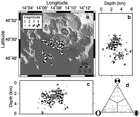
Figure 7. Campi Flegrei. Focal mechanisms dataset plotted on a shaded map (A), on a N-S (B), and an E-W (C) cross sections. (D) The distribution of focal mechanisms on a triangular Frohlich diagram (Frohlich, 1992). The dataset consists of 217 events with 0 < M < 4 occurred between 1983 and 1984.

The FPS dataset analyzed in this research consists of 217 events with 0 < M < 4 occurred between 1983 and 1984 supplied by D'Auria et al. (2014b; Figure 7). Epicenters are mainly concentrated at the axial sector of the CFc. Hypocentral depths are up to 6 km. The three extreme slip classes are well represented, with a slight prevalence of the dip-slip normal solutions (Figure 7D). The stress field has been computed applying the BRTM, using a three-dimensional grid similar to that adopted for Vesuvius: 1-km spaced nodes, for each grid node all the FPSs within a radius of 1-km have been considered for the subset inversions. Only subsets related to volumes containing at least five FPSs have been inverted (Figure 7). Results of the BRTM stress inversion procedures are shown in Figure 8 and summarized for 1, 2, and 3 km depth-slices. Only a few volumes have been inverted for the 1 km depth slice. The resulting σ₁ is high to moderately plunging and corresponds to a sub-horizontal σ₃ trending E-W. The related Φ_B values are in the range 0.5–0.8. At 2 km depth slice the attitude of the inverted σ₁ is variable, with a prevalence of sub-vertical plunges while the σ₃ trends mainly NNE-SSW. The corresponding Bishop's ratio is mainly 0.2 < Φ_B < 0.6. At 3 km depth slice the attitude of the principal stress axes is variable and the corresponding Bishop's ratio ranges from 0 to 0.8. Nevertheless at this depth too there is a prevalence of sub-vertical plunging σ₁ and a sub-horizontal NNE-SSW trending σ₃. Overall, the key features of the stress field in the area are: a nearly sub-vertical σ₁ at the center of the CFc and a low-plunging σ₁ trending radially in the surrounding areas. The corresponding σ₃ has a roughly horizontal NNE-SSW trend corresponding to the regional extensional stress field. Related Φ_B values vary between 0.3 and 0.8 (Figure 8). According to D'Auria et al. (2014b), this result is compatible with the presence of a varying stress field related to a source of deformation, located at about 2.7 km depth, that during inflation and deflation episodes (associated to an increased seismicity) is able to overcome the weak regional extensional stress field having a NNE-SSW trend.

FIGURE 8

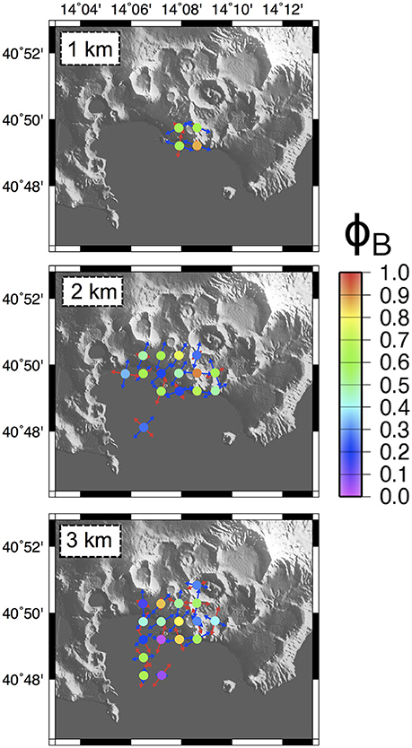
Figure 8. Campi Flegrei. Stress field tensors retrieved from focal mechanisms data using the BRTM. Slices at 1, 2, and 3 km-depth. Stress tensors have been computed over a regular grid of 1-km spacing, considering only nodes containing at least five FPSs. σ₁ and σ₃ axes are plotted as pairs of respectively red-blue arrows. The color of the circles corresponds to the retrieved Φ_B value for each node (see scale on the right).

Long Valley

Long Valley caldera (LVc) is located in eastern California at the boundary between the Sierra Nevada block and the westernmost extensional Basin And Range Province (Figure 9). LVc develops inside a transfer zone hosted between NNW-SSE trending normal faults (e.g., Dickinson, 1979; Bosworth et al., 2003). This caldera is one of the youngest volcanic systems active in California. LVc has a surface of about 500 km² and is surrounded by numerous basins and ranges (like Mammoth Mountain at SW, Glass Mountain at NE, Laurel Mountain at S). It is located near some important ENE dipping normal fault systems: Hartley Springs-Silver Lake Fault system to the North (HS, SL, in Figure 9), Hilton Creek and Round Valley Fault systems to the South (e.g., Prejean et al., 2002; Sorey et al., 2003; Bursik, 2009; HC an RV in Figure 9). Additionally, the LVc area is bounded to the east by the White Mountain Range and the related SW-dipping border faults (WMt in Figure 9). First volcanic activity can be dated approximately 760 ka ago as result of a large explosive eruption, during which more than 600 km³ of pyroclastics and ash (Bishop Tuff) have been erupted (Bailey et al., 1976). The emplacement of a resurgent dome (RD in Figure 9) located almost at the center-western sector of the caldera (started about 600 ka ago) has been causing an intense localized uplift (Hill et al., 1991; Langbein et al., 1993, 1995; Tizzani et al., 2009). Recent activity in the area consists of small eruptions and phreatic explosions at Inyo-Mono Chain (700–550 years ago; IC in Figure 9) and at Mono Lake, at NW of the LVc (about 200 years ago; Miller, 1985). Since 1978 seismicity and surface deformations have been continuously recorded in the area of the resurgent dome and in an active seismic zone along the southern margin of the caldera (Langbein, 2003). Location, size and geometry of magma bodies at LVc are still matter of debates (Carle, 1988; Battaglia et al., 1999, 2003a,b; Langbein, 2003; Tizzani et al., 2009; Guoqing, 2015). The regional active stress field in the western Basin and Range Province shows a minimum horizontal principal stress component (S_h) trending ESE-WNW, it rotates roughly to ENE-WSW at the border with the Sierra Nevada Range (Zoback, 1989, 1992; Heidbach et al., 2009). Breakout and seismic data depict a more complex pattern for the S_h across the LVc. NE-SW-trending S_h in the Resurgent Dome and at the South Moat Range, NW-SE-trending S_h in the West Moat and at Mammoth Mts. (Figure 9; Moos and Zoback, 1993; Bosworth et al., 2003, and references therein).

FIGURE 9

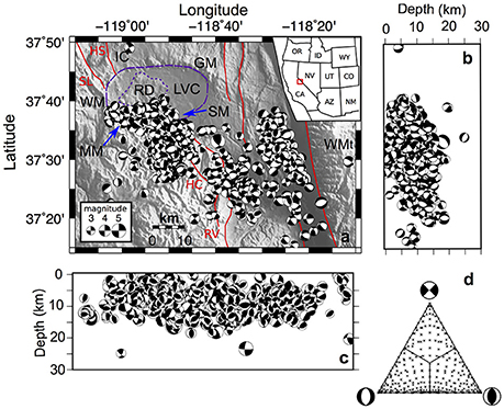
Figure 9. Long Valley. Focal mechanisms dataset plotted on a shaded map (A);, on a N-S (B), and an E-W (C) cross sections. (D) The distribution of focal mechanisms on a triangular Frohlich diagram (Frohlich, 1992). The dataset consists of 38,000 events with 0 < M < 6.4 occurred between 1978 and 2015. For sake of clarity only the events with m >= 3 are plotted. LVC, Long Valley Caldera (purple dashed line); RD, Resurgent Dome (purple dotted line); IC, Inyo Craters; WM, West Moat; MM, Mammoth Mts.; SM, South Moat; GM, Glass Mts.; WMt, White Mts. Red lines represent the main fault systems of the LVc area: SL, Silver Lake; HS, Hartley Springs Fault; HC, Hilton Creek; RV, Round Valley. See text for data sources.

For the Long Valley Caldera we used a dataset made up of about 38,000 FPSs of earthquakes occurred from 1978 to 2015 (0 < M < 6.4; Dataset by: NCEDC, 2014). These data were used to determine, with high resolution, the spatial variations of the stress field using the BRTM approach. In Figure 9 we plotted only the most energetic 3000 events (M > 3) in order to avoid an excessive overlapping of data. Epicenters are densely clustered at the southern sector of the LVc rim at the West Moat-Mammoth Mts.-South Moat Range sector. Additionally, many events are located along key tectonic lineaments of Hilton Creek and Round Valley to the south and along the western border fault of the White Mountains (Figure 9A). Hypocenters are essentially located above 20 km of depth. The shallowest events are concentrated at LVC and RD (Figures 9B,C). Kinematics of the analyzed FPSs are quite equally represented in the three main categories, with a slight prevalence of dip-slip ones (Figure 9D). The stress field has been computed on a regular three-dimensional grid of 5-km spacing. For each grid node all the FPSs within a radius of 5-km have been considered for the inversion. The stress field has been computed only at volumes containing at least 10 FPSs. Results of the stress inversion procedure are summarized in Figure 10 for depth-slices located at 0-, 10-, and 20-km. At 0 km depth slice most of the events fall in the LVc area, where the attitude of the inverted σ₁ is quite variable, with a prevalence of sub-vertical plunges (NW sector) and sub-horizontal N-S to NE-SW trends in the remaining sectors. The corresponding σ₃ is mainly sub-horizontal trending mainly E-W to NW-SE. The Bishop's ratio values are highly variable, ranging from 0.1 to 0.9. The 10 km depth slice samples most of the events of the analyzed dataset. Results can be divided up in two groups, the eastern one is dominated by a sub-horizontal σ₁ trending N-S associated to a sub-horizontal E-W trending σ₃. For the western sector, the retrieved stress field appears very similar to the one obtained for the shallowest 0-km slice; a sub-horizontal σ₁ overall trending NE-SW associated to a sub-horizontal NW-SE trending σ₃. Bishop's ratio values are highly variable ranging between 0.1 and 0.9, without a clear pattern (Figure 10). At the 20-km depth slice the stress inversion procedure highlights the presence of an overall stress field comparable to the corresponding nodes of the 10-km depth slice: in the easternmost region, a sub-horizontal NNW-SSE trending σ₁, corresponding to a sub-horizontal ENE-WSW trending σ₃. Bishop's ratios show a slight prevalence of lower values Φ_B < 0.5. Summing up, a strong background stress field seems to dominate the investigated volume: it is characterized by a sub-horizontal NNW-SSE-trending σ₁ and a sub-horizontal ENE-WSW-trending σ₃. This field is clearly evidenced by the inversion results at the deepest slices in particular at 20-km depth slice (Figure 10). The region at the south of the caldera rim experiences a clock-wise rotation of the σ₁ − σ₃ axes up to 45°, as shown at 0- and 10-km depth slices (Figure 10). Our results can be interpreted as the effect of the interaction between a background regional stress field with the local volcano-tectonic structures. The presence of two distinct stress patterns at 10-km depth slice clues the presence of a regional stress field, characterized by a sub-horizontal σ₁ roughlytrending from N-S to NNW-SSE associated with a sub-horizontal σ₃ trending from E-W to NNE-SSW. The retrieved background stress field drives the evolution of the main tectonic trends of the area (Figure 8A), overcome in the western sector by a local volcano-tectonic regime, involving mainly the shallowest lithospheric portion. This last allows the above mentioned clock-wise rotation of the σ₁ − σ₃ axes well documented at the −10-km slice (Figure 10). Our results are in agreement with S_h found in previous studies, derived by the analyses of earthquake focal mechanisms, bore-hole breakouts, fault offsets, hydraulic fracturing, and alignment of young volcanic vents. In detail, the σ₁ − σ₃ axes attitude derived for the easternmost subset inverted at −20-km slice is in good agreement with the ENE-WSW-trending S_h retrieved at the border with the Basin and Range and Sierra Nevada Range (Moos and Zoback, 1993; Prejean et al., 2002; Bosworth et al., 2003, and references therein).

FIGURE 10

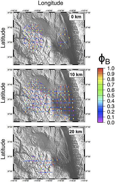
Figure 10. Long Valley. Stress field tensors retrieved from focal mechanisms data using the BRTM. Slices at 0, 10, and 20 km-depth. Stress tensors have been computed over a regular grid of 5-km spacing, considering only nodes containing at least 10 FPSs. σ₁ and σ₃ axes are plotted as pairs of respectively red-blue arrows. The color of the circles corresponds to the retrieved Φ_B value for each node (see scale on the right).

Discussion and Conclusions

In volcanic environments, a spatio-temporal analysis of the stress fields represents a valuable approach to infer the volcano dynamics (Wyss et al., 1992; Hardebeck and Michael, 2006; Gudmundsson et al., 2009; Plateaux et al., 2014; Costa and Marti, 2016). Stress field variations play a key role in driving magmas and/or fluids migration. On the other hand, injection of fluids can be responsible for local variations of the stress field allowing the reactivation of locked faults. Stress changes may influence fluid circulation within the shallow crust and they can be also responsible for the triggering of tectonic earthquakes associated to strong variations in the dynamics of volcanic eruption and behavior of hydrothermal phenomena (Linde and Sacks, 1998; Hill et al., 2002; Walter et al., 2007).

During the last decades, a wide range of stress inversion techniques has been proposed, some of them specifically conceived to manage seismological datasets. Several key aspects, that could impact on the reliability of retrieved results, require a short discussion. First of all, the discernment of the actual fault plane among the nodal planes of a FPS represents a known critical step in many analytical techniques of stress inversion. (e.g., Gephart and Forsyth, 1984; Michael, 1987; Angelier, 1990). A good solution can be an a-posteriori approach that pick the actual fault following a best-fit procedure or a massive computational approach on small datasets (Michael, 1987). Of course, it implies a complication in the processing procedure that can hide pitfalls. Only a few analytical methods do not require this choice, for instance Angelier (2002) based on the slip shear component criterion. Additionally, all graphical (e.g., RDM) or graphical-derived (e.g., RTM, BRTM) techniques do not require this pre-selection; this is a valuable asset that makes these processing approaches as robust as they are simple. As premised, graphical-derived methods are based on the implementation of an algorithm that is able to figure a probability function over the focal sphere for both σ₁ and σ₃ principal stress attitude. The analytical implementation of the classical graphical methods allows the efficient managing of large datasets following a proper statistical approach (e.g., RDTM; Ramsay and Lisle, 2000). Generally, the output of these procedures needs a strong graphical post-processing in order to obtain an adequate representation of results (e.g., MORE; Massa, 2003). BRTM proposes a solution to this limitation offering a standard procedure of data ingestion, processing and graphical post-processing in both 2- and 3-Dimensional rendering. All these task can be performed through the use of editable scripts run in the same computational environment. A known drawback of stress inversion procedures (for both graphical and analytical) is that they generally lack of a robust statistical estimation of the uncertainty on the retrieved tensors. To overcome this lack, BRTM performs an estimation of solution uncertainty and trough the implementation of the approach of Jackson and Matsu'ura (1985), BRTM is able to delimit the confidence intervals around the σ1 and σ3 retrieved axes (D'Auria and Massa, 2015). Another key aspect to consider is that very frequently datasets to be processed are large and heterogeneous. Without an a-priori selection, many datasets collect faults/FPS related to different stress fields. For instance, seismological datasets collected across wide lithospheric volume, mesoscale faults hosted in a limited rock volume but generated during different tectonic events, etc. The solution to identify the different contributions from multiple sources can be a clustering approach as the MIM (Yamaji, 2000; Otsubo et al., 2008) or the application of other automatic analytical procedures (Angelier and Manoussis, 1980). These approaches allows the identification of the different stress fields but they are not designed to give a quantitative assessment of the solution quality; additionally they are not able to locate the spatial distribution of the retrieved tensors (Yamaji, 2000; D'Auria and Massa, 2015). The relevance of this point becomes larger considering the seismological datasets collected in volcanic areas. Here, the retrieving of stress field spatial variations represents a crucial task: sensible variation in stress axes attitude can characterize stress field active in contiguous volumes (e.g., D'Auria et al., 2014a,b; Plateaux et al., 2014). For this reason, unsupervisioned stress inversions performed on an unselected dataset can be quite useless. A similar discussion can be done for the analysis of stress field temporal variations. The ideal way to obtain a reliable stress field inversion would be the analysis of a dataset covering a time interval as short as possible, in order to consider the responsible stress field quite constant in its parameters (i.e., the attitude of principal stress axes and the related Φ_B). The preliminary temporal selection of data can be unfeasible in case of mesoscale faults also when collected in a limited volume of rock: several tectonic “phases” could have superimposed in the geological record. Conversely, the temporal selection of data can be conveniently done in the analysis of seismological datasets where the focal parameters are well known. In volcanic environments, a spatio-temporal analysis of the stress fields represents the best way to infer about the volcano dynamics (Wyss et al., 1992; Hardebeck and Michael, 2006; D'Auria et al., 2014b; Plateaux et al., 2014). In this perspective, a supervisioned splitting of data in 3D sub-volumes represents the best solution to retrieve the spatial distribution of active coeval stress fields. As a final consideration about the stress inversion procedures, it should be noted that the publication of a rigorous formulation of a technique is not enough to determine its success. A strong limitation to the dissemination of a processing procedure consists of the availability of a free or open-source platform of implementation. Available methods are frequently implemented by authors and freely distributed to the community only as PC programs. For instance, the Direct Inversion algorithm was implemented by the author in the executing software TENSOR (Angelier, 1990), the Multiple Inverse Method can be performed through a set of executable supplied by the author (Yamaji, 2000), RDM and RTM can be applied using RDTM, supplied by authors both as executing program than as code (Ramsay and Lisle, 2000). The availability of an editable code represents a key point to allow a flexible use of a technique, allowing, in addition, a facilitation in its spreading over the community. A BRTM implementation in MATLAB^® was proposed by the Authors, allowing a basic stress-inversion procedure and an advanced plot of results (Figure 3; D'Auria and Massa, 2015). The implementation of the basic inversion algorithm can be easily exported to open-source and free platform. Results can be plotted using the preferred platform. The graphical post-processing proposed by D'Auria and Massa (2015) was implemented in MATLAB^®. It would be useful a revision in order to make it available to free platforms.

According to previous researches, the new stress-inversions discussed in this paper (Figures 6, 8, 10), have shown that the stress field in the studied volcanoes results from the interaction of a regional background field with local volcanic structures and dynamics. In detail, during the 1983–1984 seismic crisis in the Campi Flegrei area, a sub-vertical σ₁ dominates the axial volume of the caldera. Conversely, a low-plunging σ₁ appears trending radially in the surrounding volumes. The corresponding σ₃ attitudes are roughly sub-horizontal NNE-SSW trending, in accordance with the regional S_h retrieved by breakout data (Montone et al., 2012). The retrieved stress fields are in accordance with Zuppetta and Sava (1991). The background regional stress field has been also modeled by D'Auria et al. (2014b) using a joint inversion of a geodetical-seismological dataset, obtaining a sub-horizontal σ₃ trending N-S. This result is in good accordance with the Mt. Somma-Vesuvius where D'Auria et al. (2014a) found a very similar configuration for the regional stress field. The retrieved variability of the stress field can be related to fluids migration within a planar crack probably located at shallow depth and possibly responsible for unrest episodes (D'Auria et al., 2014b; Macedonio et al., 2014). At Mt. Vesuvius, rheological variations of the involved geological units and the action of key volcano-tectonic structures seem to play a significant role in determining the local stress fields (Figures 4–6; D'Auria et al., 2014a). The configuration of the retrieved stress fields shows the superposition of two volumes with a marked difference in their evolution history. A top volume dominated by a gravitational volcanic spreading that allows the setting of extensional stress fields (low Φ_B values and sub-vertical σ₁) active in the analyzed sub-volumes. A bottom volume strictly related to a regional extensional background stress field in accordance with the S_h derived by breakout data (Figure 6; Borgia et al., 2005; Montone et al., 2012; D'Auria et al., 2014a). The computation of the stress field using the BRTM on a regular three-dimensional grid allows the 3-D figuration of the stress fields “simultaneously” acting from the surface to about 8-km depth (Figures 5, 6). This approach appears very useful in supporting studies on the volcano-dynamics of complex system as the Mt. Somma-Vesuvius. Finally, analyses performed at Long Valley Caldera show a complex configuration of the stress field pattern associated to a volcanic district developed inside a transfer zone hosted between NNW-SSE trending normal faults (e.g., Dickinson, 1979; Bosworth et al., 2003). A dataset of 38,000 FPSs allows to retrieve with high resolution, the spatial variations of the stress field active in the first 20 km of depth. A regional background stress field dominates the deepest portion of the investigated volume accordingly to the ENE-WSW-trending S_h retrieved at the border with the Basin and Range and Sierra Nevada Range (Moos and Zoback, 1993; Prejean et al., 2002; Bosworth et al., 2003). In the shallowest lithospheric portions this regional stress field has been overcome by the volcano-tectonic regime; this is clear in particular at the 10 km depth-slice (Figures 9, 10). The managing of the very large dataset has been approached using a regular sampling of data inverted using the BRTM. The result is a very detailed figuration of the spatial variation of the active stress fields in the 500 km² Long Valley Caldera, one of the youngest volcanic systems active in California.

The above results confirm that the application of stress inversion procedures to volcanic environments provides crucial information about the volcano dynamics with particular care to its interaction with regional tectonics. In detail, BRTM has shown to be very efficient in managing heterogeneous datasets in a user-friendly processing environment, with a clear graphic output and an efficient evaluation of the regions of confidence around the retrieved principal stress axes. The proposed processing approach of FPS datasets in active volcanic areas is suitable to be applied to a wide range of contexts. Finally, the results presented in this work suggest that these methods could be useful also as a near real-time monitoring tool to characterize spatial and temporal variations in the stress field linked to a volcanic unrest (e.g., Toda et al., 2002; Plateaux et al., 2014). A final consideration concerns the relevance of the stress-inversion approach based on the integration and/or the joint inversion of seismological and geodetical datasets. The joint inversion of ground deformation and focal mechanism is more efficient than the mere comparison of the results obtained by the separate inversion (Segall, 2013; D'Auria et al., 2014b; Viccaro et al., 2016). Spatial-temporal analysis of the stress field derived from seismological datasets associated to a continuous recording of ground deformations (remote and/or field classical techniques) could be a reliable tool to monitor volcano dynamics and infer about their evolution.

Author Contributions

BM, LD, EC, and AD: rock mechanics, stress inversion, join inversion, and focal mechanisms.

Funding

This research is financially supported by: MED-SUV project (European Union's Seventh Programme for research, technological development and demonstration, Grant Agreement Number 308665); Università degli Studi del Sannio FRA 2014–2015 “Modeling of geological processes” (P.I. B. Massa).

Conflict of Interest Statement

The authors declare that the research was conducted in the absence of any commercial or financial relationships that could be construed as a potential conflict of interest.

The handling Editor declared a shared affiliation, though no other collaboration, with the authors BM, LD, and EC and states that the process nevertheless met the standards of a fair and objective review.

Acknowledgments

Thanks are due to the two Referees, Eisuke Fujita and Mimmo Palano, to the Associate Editor Antonio Costa and to the Chief Editor Valerio Acocella for the constructive and valuable review that greatly improved the manuscript. BRTM can be accessed as Electronic Supplement to D'Auria and Massa (2015) following the link: http://srl.geoscienceworld.org/content/early/2015/03/17/0220140153 (Last accessed on 31st October 2016).

References

Acocella, V., and Funiciello, R. (2006). Transverse systems along the extensional Tyrrhenian margin of central Italy their influence on volcanism. Tectonics, 25:TC2003. doi: 10.1029/2005TC001845

CrossRef Full Text | Google Scholar

Andronico, D., Calderoni, G., Cioni, R., Sbrana, A., Sulpizio, R., and Santacroce, R. (1995). Geological map of Somma-Vesuvius volcano. Period. Mineral. 64, 77–78.

Angelier, J. (1990). Inversion of field data in fault tectonics to obtain the regional stress. III—A new rapid direct inversion method by analytical means. Geophys. J. Int. 103, 363–376. doi: 10.1111/j.1365-246X.1990.tb01777.x

CrossRef Full Text | Google Scholar

Angelier, J. (2002). Inversion of earthquake focal mechanisms to obtain the seismotectonic stress IV—A new method free of choice among nodal planes. Geophys. J. Int. 150, 588–609. doi: 10.1046/j.1365-246X.2002.01713.x

CrossRef Full Text | Google Scholar

Angelier, J., and Baruah, S. (2009). Seismotectonics in Northeast India: a stress analysis of focal mechanism solutions of earthquakes and its kinematic implications. Geophys. J. Int. 178, 303–326. doi: 10.1111/j.1365-246X.2009.04107.x.

CrossRef Full Text | Google Scholar

Angelier, J., and Manoussis, S. (1980). Classification automatique et distinction de phases superposées en tectonique cassante. C. R. Acad. Sci. Paris 290, 651–654.

Angelier, J., and Mechler, P. (1977). Sur une méthode graphique de recherche des contraintes principales également utilisable en tectonique et en séismologie: La méthode des diédres droits. Bulletin de la SocieÌĄteÌĄ GeÌĄologique de France 19, 1309–1318.

Bailey, R. A., Dalrymple, G. B., and Lanphere, M. A. (1976). Volcanism, structure and geochronology of Long Valley caldera, Mono County, California. J. Geophys. Res. 81, 725– 744. doi: 10.1029/JB081i005p00725

CrossRef Full Text | Google Scholar

Battaglia, M., Roberts, C., and Segall, P. (1999). Magma intrusion beneath Long Valley caldera confirmed by temporal changes in gravity. Science 285, 2119–2122. doi: 10.1126/science.285.5436.2119

PubMed Abstract | CrossRef Full Text | Google Scholar

Battaglia, M., Segall, P., Murray, J., Cervell, P., and Langbein, J. (2003a). The mechanics of unrest at Long Valley caldera, California: 1. Modeling the geometry of the source using GPS, leveling and two-color EDM data. J. Volcanol. Geother. Res. 127, 195–217. doi: 10.1016/S0377-0273(03)00170-7

CrossRef Full Text | Google Scholar

Battaglia, M., Segall, P., and Roberts, C. (2003b). The mechanics of unrest at Long Valley caldera, California. 2. Constraining the nature of the source using geodetic and micro-gravity data. J. Volcanol. Geother. Res. 127, 219–245. doi: 10.1016/S0377-0273(03)00171-9

CrossRef Full Text | Google Scholar

Bernasconi, A., Bruni, P., Gorla, L., Principe, C., and Sbrana, A. (1981). Risultati preliminari dell'esplorazione geotermica profonda nell'area vulcanica del Somma-Vesuvio. Rend. Soc. Geol. 4, 237–240.

Bianco, F., Castellano, M., Milano, G., Ventura, G., and Vilardo, G. (1998). The Somma-Vesuvius stress field induced by regional tectonics: evidences from seismological and mesostructural data. J. Volcanol. Geother. Res. 82, 119–218. doi: 10.1016/S0377-0273(97)00065-6

CrossRef Full Text | Google Scholar

Bishop, A. (1966). The strength of solids as engineering materials. Geotechnique 16, 91–130. doi: 10.1680/geot.1966.16.2.91

CrossRef Full Text | Google Scholar

Borgia, A., Tizzani, P., Solaro, G., Manzo, M., Casu, F., Luongo, et al. (2005). Volcanic spreading of Vesuvius, a new paradigm for interpreting its volcanic activity. Geophys. Res. Lett. 32:L03303, doi: 10.1029/2004GL022155

CrossRef Full Text

Bosworth, W., Burke, K., and Strecker, M. (2003). Effect of stress fields on magma chamber stability and the formation of collapse calderas. Tectonics 22:1042.

Google Scholar

Bott, M. (1959). The mechanisms of oblique slip faulting. Geol. Mag. 96, 109–117.

Google Scholar

Brocchini, D., Principe, C., Castradori, D., Laurenzi, M. A., and Gorla, L. (2001). Quaternary evolution of the southern sector of the Campania Plain and early Somma-Vesuvius activity: insights from the Trecase 1 well. Mineral. Petrol. 73, 67–91. doi: 10.1007/s007100170011

CrossRef Full Text | Google Scholar

Bursik, M. (2009). A general model for tectonic control of magmatism: Examples from Long Valley Caldera (USA) and El Chichón (México). Geofísica Int. 48, 171–183. Available online at: http://www.scielo.org.mx/pdf/geoint/v48n1/v48n1a12.pdf

Byerly, P. (1928). The nature of the first motion in the Chilean earthquake of November 11, 1922. Am. J. Sci. 16, 232–236. doi: 10.2475/ajs.s5-16.93.232

CrossRef Full Text | Google Scholar

Cannavò, F., Scandura, D., Palano, M., and Musumeci, C. (2014). A joint inversion of ground deformation and focal mechanisms data for magmatic source modelling. Pure Appl. Geophys. 171, 1695–1704. doi: 10.1007/s00024-013-0771-x

CrossRef Full Text | Google Scholar

Carey, E., and Brunier, B. (1974). Analyse théorique et numérique d'un modéle mécanique élémentaire appliquéăá l'étude d'une population de failles. C. R. Acad. Sci. D179, 891–894.

Carey-Gailhardis, E., and Mercier, J. (1987). A numerical method for de- termining the state of stress using focal mechanisms of earthquake populations: application to Tibetan teleseisms and microseismicity of southern Peru. Earth Planet. Sci. Lett. 82, 165–179. doi: 10.1016/0012-821X(87)90117-8

CrossRef Full Text | Google Scholar

Carey-Gailhardis, E., and Mercier, J. L. (1992). Regional state of stress, fault kinematics and adjustments of blocks in a fractured body of rock: application to the micro-seismicity of the Rhine graben. J. Struct. Geol. 14, 1007–1017. doi: 10.1016/0191-8141(92)90032-R

CrossRef Full Text | Google Scholar

Carle, S. F. (1988). Three-dimensional gravity modeling of the geologic structure of Long Valley Caldera. J. Geophys. Res. 93, 13237–13250. doi: 10.1029/jb093ib11p13237

CrossRef Full Text | Google Scholar

Chiodini, G. L., Marini, M., and Russo (2001). Geochemical evidence for the existence of high-temperature hydrothermal brines at Vesuvio volcano, Italy. Geochim. Cosmochim. Acta 65, 2129–2147. doi: 10.1016/S0016-7037(01)00583-X

CrossRef Full Text

Cocina, O., Neri, G., Privitera, E., and Spampinato, S. (1997). Stress tensor computations in the Mount Etna area (Southern Italy) and tectonic implications. J. Geodynamics 23, 109–127. doi: 10.1016/S0264-3707(96)00027-0

CrossRef Full Text | Google Scholar

Costa, A., and Marti, J. (2016). Stress field control during large caldera-forming eruptions. Front. Earth Sci. 4:92, doi: 10.3389/feart.2016.00092

CrossRef Full Text | Google Scholar

D'Auria, L., Esposito, A. M., Lo Bascio, D., Ricciolino, P., Giudicepietro, F., Martini, M., et al. (2013). The recent seismicity of Mt. Vesuvius: inference on seismogenic processes. Ann. Geophys. 56:S0442, doi: 10.4401/ag-6448

CrossRef Full Text | Google Scholar

D'Auria, L. F., Giudicepietro, I., Aquino, G., Borriello, C., Del Gaudio, D., Lo Bascio, M., et al. (2011). Repeated fluid-transfer episodes as a mechanism for the recent dynamics of Campi Flegrei caldera (1989–2010). J. Geophys. Res. 116:B04313, doi: 10.1029/2010JB007837

CrossRef Full Text

D'Auria, L., Martini, M., Esposito, A., Ricciolino, P., and Giudicepietro, F. (2008). “A unified 3D velocity model for the Neapolitan volcanic areas,” in Conception, Verification and Application of Innovative Techniques to Study Active Volcanoes, eds W. Marzocchi and A. Zollo (Napoli: INGV-DPC), 375–390.

D'Auria, L., and Massa, B. (2015). Stress inversion of focal mechanism data using a bayesian approach: a novel formulation of the right trihedra method. Seism. Res. Lett. 86, 968–977. doi: 10.1785/0220140153

CrossRef Full Text | Google Scholar

D'Auria, L., Massa, B., Cristiano, E., Del Gaudio, C., Giudicepietro, F., Ricciardi, G., et al. (2014b). Retrieving the stress field within the campi flegrei caldera (southern italy) through an integrated geodetical and seismological approach. Pure Appl. Geophy. 172, 3247–3263. doi: 10.1007/s00024-014-1004-7

CrossRef Full Text | Google Scholar

D'Auria, L., Massa, B., and De Matteo, A. (2014a). The stress field beneath a quiescent stratovolcano: the case of mount Vesuvius. J. Geophys. Res. 119, 1181–1199. doi: 10.1002/2013JB010792

CrossRef Full Text | Google Scholar

Deino, A. L., Orsi, G., Piochi, M., and De Vita, S. (2004). The age of the neapolitan Yellow Tuff caldera-forming eruption (Campi Flegrei caldera–Italy) assessed by 40ar/39ar dating method. J. Volcanol. Geother. Res. 133, 157–170. doi: 10.1016/S0377-0273(03)00396-2

CrossRef Full Text | Google Scholar

Del Gaudio, C., Aquino, I., Ricciardi, G. P., Ricco, C., and Scandone, R. (2010). Unrest episodes at Campi Flegrei: a reconstruction of vertical ground movements during 1905–2009. J. Volcanol. Geother. Res. 195, 48–56. doi: 10.1016/j.jvolgeores.2010.05.014

CrossRef Full Text | Google Scholar

De Matteis, R., Matrullo, E., Rivera, L., Stabile, T. A., Pasquale, G., and Zollo, A. (2012). Fault Delineation and Regional Stress Direction from the Analysis of Background Microseismicity in the southern Apennines, Italy. Bull. Seismol. Soc. Am. 102, 1899–1907. doi: 10.1785/0120110225

CrossRef Full Text | Google Scholar

Dickinson, W. R. (1979). “Cenozoic plate tectonic setting of the Cordilleran region in the United States,” in Pacific Coast Paleogeography Symposium 3; Cenozoic Paleogeography of the Western United States, eds J. M. Armentrout, M. R. Cole, and H. TerBest Jr. (Anaheim, CA: Pac. Sect., Soc. of Econ, Paleontol. and Mineral), 1–13.

Di Vito, M. A., Isaia, R., Orsi, G., Southon, J., De Vita, S., D'antonio, M., et al. (1999). Volcanism and deformation since 12,000 years at the Campi Flegrei caldera (Italy). J. Volcanol. Geother. Res. 91, 221–246. doi: 10.1016/S0377-0273(99)00037-2

CrossRef Full Text | Google Scholar

Frohlich, C. (1992). Triangle diagrams: ternary graphs to display similarity and diversity of earthquake focal mechanisms. Phys. Earth. Planet. Inter. 75, 193–198. doi: 10.1016/0031-9201(92)90130-N

CrossRef Full Text | Google Scholar

Gebauer, S., Schmitt, A. K., Pappalardo, L., Stockli, D. F., and Lovera, O. M. (2014). Crystallization and eruption ages of Breccia Museo (Campi Flegrei caldera, Italy) plutonic clasts and their relation to the Campanian ignimbrite. Contrib. Mineral. Petrol. 167:953. doi: 10.1007/s00410-013-0953-7

CrossRef Full Text | Google Scholar

Gephart, J., and Forsyth, D. (1984). An improved method for determining the regional stress tensor using earthquake focal mechanism data: application to the San Fernando earthquake sequence. J. Geophys. Res. 89, 9305–9320. doi: 10.1029/JB089iB11p09305

CrossRef Full Text | Google Scholar

Gillard, D., and Wyss, M. (1995). Comparison of strain and stress tensor orientation: application to Iran and southern California. J. Geophys. Res. 100, 22197–22213. doi: 10.1029/95JB01871

CrossRef Full Text | Google Scholar

Giudicepietro, F., Orazi, M., Scarpato, G., Peluso, R., D'Auria, L., Ricciolino, P., et al. (2010). Seismological monitoring of Mount Vesuvius (Italy): more than a century of observations. Seism. Res. Lett. 81, 625–634, doi: 10.1785/gssrl.81.4.625

CrossRef Full Text | Google Scholar

Guoqing, L. (2015). Seismic velocity structure and earthquake relocation for the magmatic system beneath Long Valley Caldera, eastern California. J. Volcanol. Geother. Res. 296, 19–30. doi: 10.1016/j.jvolgeores.2015.03.007

CrossRef Full Text | Google Scholar

Gudmundsson, A., Acocella, V., and Vinciguerra, S. (2009). Understanding stress and deformation in active volcanoes. Tectonophysics 471, 1–3. doi: 10.1016/j.tecto.2009.04.014

CrossRef Full Text

Hardebeck, J. L., and Hauksson, E. (2001). Stress orientations obtained from earthquake focal mechanisms: what are appropriate uncertainty estimates? Bull. Seismol. Soc. Am. 91, 250–252. doi: 10.1785/0120000032

CrossRef Full Text | Google Scholar

Hardebeck, J. L., and Michael, A. J. (2006). Damped regional-scale stress inversions: methodology and examples for southern California and the Coalinga aftershock sequence. J. Geophys. Res. 111:B11310, doi: 10.1029/2005JB004144

CrossRef Full Text | Google Scholar

Heidbach, O., Tingay, M., Barth, A., Reinecker, J., and Kurfeß, D. and Müller, B. (2009). The World Stress Map based on the database release 2008, equatorial scale 1:46,000,000. Paris: Commission for the Geological Map of the World.

Hill, D. P., Johnston, M. J. S., Langbein, J. O., McNutt, S. R., Miller, C. D., Mortensen, C. E., et al. (1991). Response Plans for Volcanic Hazards in the Long Valley Caldera and Mono Craters area, California. Open-File Report, U.S. Geology Survey.

Hill, D. P., Pollitz, F., and Newhall, C. (2002). Earthquake-volcano interactions. Phys. Today 55, 41–47. doi: 10.1063/1.1535006

CrossRef Full Text | Google Scholar

Ippolito, F., Ortolani, F., and Russo, M. (1973). Struttura marginale tirrenica dell'Appennino campano: reinterpretazione di dati di antiche ricerche di idrocarburi. Mem. Soc. Geol. 12, 227–250.

Jackson, D. D., and Matsu'ura, M. (1985). A Bayesian approach to nonlinear inversion. J. Geophys. Res. 90, 581–591. doi: 10.1029/JB090iB01p00581

CrossRef Full Text | Google Scholar

Langbein, J. O. (2003). Deformation of the Long Valley caldera, California: inferences from measurements from 1988 to 2001. J. Volcanol. Geother. Res. 127, 247–267. doi: 10.1016/S0377-0273(03)00172-0

CrossRef Full Text | Google Scholar

Langbein, J. O., Dzurisin, D., Marshall, G., Stein, R., and Rundle, J. (1995). Shallow and peripheral volcanic sources of inflativo revealed by modeling two-color geodimeter and leveling data from Long Valley caldera, California, 1988–1992. J. Geophys. Res. 100, 12487–12495. doi: 10.1029/95JB01052

CrossRef Full Text

Langbein, J. O., Hill, D. P., Parker, T. N., and Wilkinson, S. K. (1993). An episode of re-inflation of the Long Valley caldera, eastern California, 1989–1991. J. Geophys. Res. 98, 15851–15870. doi: 10.1029/93JB00558

CrossRef Full Text | Google Scholar

Lavecchia, G., Boncio, P., Creati, N., and Brozzetti, F. (2003). Some aspects of the Italian geology not fitting with a subduction scenario. J. Virtual Explor. 10, 1–42. doi: 10.3809/jvirtex.2003.00064

CrossRef Full Text | Google Scholar

Linde, A. T., and Sacks, I. S. (1998). Triggering of volcanic eruptions. Nature 395, 888–890. doi: 10.1038/27650

CrossRef Full Text | Google Scholar

Lisle, R. (1988). ROMSA: a basic program for paleostress analysis using fault striation data. Comput. Geosci. 14, 255–259. doi: 10.1016/0098-3004(88)90007-6

CrossRef Full Text | Google Scholar

Lisle, R. J. (1987). Principal stress orientations from faults: an additional constraint. Annales Tectonicae 1, 155–158.

Google Scholar

Lomax, A., Zollo, A., Capuano, P., and Virieux, J. (2001). Precise, absolute earthquake location under Somma-Vesuvius volcano using a new three-dimensional velocity model. Geophys. J. Int. 146, 313–331. doi: 10.1046/j.0956-540x.2001.01444.x

CrossRef Full Text | Google Scholar

Macedonio, G., Giudicepietro, F., D'auria, L., and Martini, M. (2014). Sill intrusion as a source mechanism of unrest at volcanic calderas. J. Geophys. Res. Solid Earth 119, 3986–4000. doi: 10.1002/2013JB010868

CrossRef Full Text | Google Scholar

Massa, B. (2003). Relazione Tra Faglie Quaternarie e Sismicita NellŠarea Sannita, Printed, Dottorato di Ricerca in Scienze della Terra e della Vita, XV ciclo., Universita degli Studi del Sannio, Benevento, Italy.

Michael, A. J. (1987). Use of Focal Mechanisms to Determine Stress: a control study. J. Geophys. Res. 92, 357–368. doi: 10.1029/JB092iB01p00357

CrossRef Full Text | Google Scholar

Milia, A., Torrente, M. M., Massa, B., and Iannace, P. (2013). Progressive changes in rifting directions in the Campania margin (Italy): New constrains for the Tyrrhenian Sea opening. Global Planetary Change 109, 3–17. doi: 10.1016/j.gloplacha.2013.07.003

CrossRef Full Text | Google Scholar

Miller, C. D. (1985). Holocene eruptions at the Inyo volcanic chain, California: implications for possible eruptions in Long Valley caldera. Geology 13, 14–17. doi: 10.1130/0091-7613(1985)13<14:HEATIV>2.0.CO;2

CrossRef Full Text | Google Scholar

Montone, P., Mariucci, M. T., and Pierdominici, S. (2012). The Italian present-day stress map. Geophys. J. Int. 189, 705–716, doi: 10.1111/j.1365-246X.2012.05391.x

CrossRef Full Text | Google Scholar

Moos, D., and Zoback, M. D. (1993). State of stress in the Long Valley caldera, California. Geology 21, 837–840. doi: 10.1130/0091-7613(1993)021<0837:SOSITL>2.3.CO;2

CrossRef Full Text | Google Scholar

NCEDC (2014). Northern California Earthquake Data Center. Berkeley: UC Berkeley Seismological Laboratory. Dataset.

Otsubo, M., Yamaji, A., and Kubo, A. (2008). Determination of stresses from heterogeneous focal mechanism data: an adaptation of the multiple inverse method. Tectonophysics 475, 150–160. doi: 10.1016/j.tecto.2008.06.012

CrossRef Full Text | Google Scholar

Pedersen, R., and Sigmundsson, F. (2004). InSAR based sill model links spatially offset areas of deformation and seismicity for the 1994 unrest episode at Eyjafjallajökull volcano, Iceland. Geophys. Res. Lett. 31:L14610. doi: 10.1029/2004GL020368

CrossRef Full Text | Google Scholar

Plateaux, R., Béthoux, N., Bergerat, F., and Mercier de Lépinay, B. (2014). Volcano-tectonic interactions revealed by inversion of focal mechanisms: stress field insight around and beneath the Vatnajökull ice cap in Iceland. Front. Earth Sci. 2:9, 1–21. doi: 10.3389/feart.2014.00009

CrossRef Full Text

Prejean, S., Ellsworth, W., Zoback, M., and Walhouser, F. (2002). Fault structure and kinematics of the Long Valley Caldera region, California, revealed by high-accuracy earthquake hypocenters and focal mechanism stress inversion. J. Geophys. Res. 107:2355, doi: 10.1029/2001JB001168

CrossRef Full Text | Google Scholar

Ramsay, J., and Lisle, R. (2000). The Techniques of Modern Structural Geology, Volume 3: Applications of Continuum Mechanics in Structural Geology. London: Academic Press.

Google Scholar

Reasenberg, P., and Oppenheimer, D. (1985). FPFIT, FPPLOT and FPPAGE: Fortran Computer Programs for Calculating and Displaying Earthquake Fault Plane Solutions. Open File Report U.S. Geological Survey.

Reid, H. F. (1910). “The mechanism of the earthquake,” in The California Earth-quake of April 18, 1906. Report of the State Earthquake Investigation Commission, Vol. 2 (Washington, DC: Carnegie Institution for Science), 1–192.

Rivera, L., and Cisternas, A. (1990). Stress tensor and fault plane solutions for a population of earthquakes. Bull. Seismol. Soc. Am. 80, 600–614.

Google Scholar

Rosi, M., Santacroce, R., and Sbrana, A. (1987). Geological Map of the Somma-Vesuvius Volcanic Complex (Scale 1:25000). Roma: CNR,PF Geodinamica, L Salomone.

Google Scholar

Santacroce, R. (ed.). (1987). Somma-Vesuvius, Vol. 114, Rome: CNR.

Segall, P. (2013). Volcano Deformation and Eruption Forecasting. London: Geological Society; Special Publications.

Google Scholar

Sorey, M. L., McConnell, V. S., and Roeloffs, E. (2003). Summary of recent research in Long Valley caldera, California. J. Volcanol. Geother. Res. 127, 165–173. doi: 10.1016/S0377-0273(03)00168-9

CrossRef Full Text | Google Scholar

Tizzani, P., Battaglia, M., Zeni, G., Atzori, S., Berardino, P., and Lanari, R. (2009). Uplift and magma intrusion at Long Valley caldera from InSAR and gravity measurements. Geology 37, 63–66. doi: 10.1130/G25318A.1

CrossRef Full Text | Google Scholar

Toda, S., Stein, R. S., and Sagiya, T. (2002). Evidence from the AD 2000 Izu islands earthquake swarm that stressing rate governs seismicity. Nature 419, 58–61. doi: 10.1038/nature00997

PubMed Abstract | CrossRef Full Text | Google Scholar

Umakoshi, K., Shimizu, H., and And Matsuwo, N. (2001). Volcano-tectonic seismicity at Unzen Volcano, Japan, 1985–1999. J. Volcanol. Geother. Res. 112, 117–131. doi: 10.1016/S0377-0273(01)00238-4

CrossRef Full Text | Google Scholar

Ventura, G., and Vilardo, G. (1999). Slip tendency analysis of the Vesuvius faults: implication for the seismotectonic and volcanic hazard assessment. Geophys. Res. Lett. 26, 3229–3232. doi: 10.1029/1999GL005393

CrossRef Full Text | Google Scholar

Viccaro, M., Zuccarello, F., Cannata, A., Palano, M., and Gresta, S. (2016). How a complex basaltic volcanic system works: constraints from integrating seismic, geodetic, and petrological data at Mount Etna volcano during the July-August 2014 eruption. J. Geophys. Res. Solid Earth 121, 5659–5678. doi: 10.1002/2016JB013164

CrossRef Full Text | Google Scholar

Vitale, S., and Isaia, R. (2013). Fractures and faults in volcanic rocks (Campi Flegrei, southern Italy): insight into volcano-tectonic processes. Int. J. Earth Sci. 103, 801–819. doi: 10.1007/s00531-013-0979-0

CrossRef Full Text | Google Scholar

Wallace, R. E. (1951). Geometry of shearing stress and relation to faulting. J. Geol. 22, 118–130. doi: 10.1086/625831

CrossRef Full Text | Google Scholar

Walter, T. R., Wang, R., Zimmer, M., Grosser, H., Luhr, B., and Ratdomopurbo, A. (2007). Volcanic activity influenced by tectonic earthquakes: static and dynamic stress triggering at Mt. Merapi. Geophys. Res. Lett. 34:L05304. doi: 10.1029/2006gl028710

CrossRef Full Text | Google Scholar

Wyss, M., Liang, B., Tanigawa, W. R., and Xiaoping, W. (1992). Comparison of orientations of stress and strain tensor based on fault plane solutions in Kaoiki, Hawaii. J. Geophys. Res. 97, 4769–4790. doi: 10.1029/91JB02968

CrossRef Full Text | Google Scholar

Yamaji, A. (2000). The multiple inverse method: a new technique to separate stresses from heterogeneous fault-slip data. J. Struct. Geol. 22, 441–452. doi: 10.1016/S0191-8141(99)00163-7

CrossRef Full Text | Google Scholar

Yamaji, A. (2007). An Introduction to Tectonophysics: Theoretical Aspects of Structural Geology. Tokyo: TERRAPUB.

Google Scholar

Zoback, M. L. (1989). State of stress and modern deformation of the northern basin and rangeprovince. J. Geophys. Res. 94, 7105–7128. doi: 10.1029/JB094iB06p07105

CrossRef Full Text | Google Scholar

Zoback, M. L. (1992). First and second-order patterns of stress in the lithosphere: the world stress map project. J. Geophys. Res. 97, 11703–11728. doi: 10.1029/92JB00132

CrossRef Full Text | Google Scholar

Zollo, A., Marzocchi, W., Capuano, P., Lomax, A., and Iannaccone, G. (2002). Space and time behaviour of seismic activity and Mt. Vesuvius volcano, Southern Italy. Bull. Seismol. Soc. Am. 92, 625–640. doi: 10.1785/0120000287

CrossRef Full Text | Google Scholar

Zuppetta, A., and Sava, A. (1991). Stress pattern at Campi Flegrei from focal mechanisms of the 1982–1984 earthquakes (Southern Italy). J. Volcanol. Geother. Res. 48, 127–137. doi: 10.1016/0377-0273(91)90038-2

CrossRef Full Text | Google Scholar