An Empirical Approach for Estimating Stress-Coupling Lengths for Marine-Terminating Glaciers

Introduction

Dynamic mass loss from Greenland's marine-terminating glaciers accounted for nearly half of the ice sheet's mass loss over the last two decades (Enderlin et al., 2014) yet the processes controlling the timing and magnitude of changes in dynamics are poorly understood (Vieli and Nick, 2011). Force balance estimates (van der Veen and Whillans, 1989), constrained with surface observations, potentially offer insight into the spatial and temporal variations in driving and resistive stresses that govern glacier flow. However, poor spatial coverage, low resolution, and large uncertainties in velocity and thickness have historically limited its application to a handful of glaciers (e.g., Whillans et al., 1989; O'Neel et al., 2005; Kavanaugh and Cuffey, 2009; Sergienko and Hindmarsh, 2013; van der Veen et al., 2014). Moreover, differences in the way that observational datasets have been incorporated into analyses have thus far prevented rigorous comparisons of how different glaciers respond to common environmentally-forced stress perturbations.

Recent advances in observational technology have increased the accuracy and spatial coverage of radar-derived bed elevation estimates and decreased the temporal repeat interval of surface velocity and elevation observations. These improvements have vastly expanded the potential to investigate differences in glacier dynamics using analytical and numerical modeling techniques. To take advantage of the increased availability of high-resolution surface observations, the processing of these input data must be carefully considered. A key consideration is the distance over which stresses are horizontally transferred within glacier ice (Kamb and Echelmeyer, 1986; Bahr et al., 1994; O'Neel et al., 2005; Maxwell et al., 2008), i.e., the stress-coupling length (hereafter referred to as the SCL). Because of stress coupling, glaciers act as low-pass filters, limiting the spatial scales over which stress perturbations at the bed will be expressed at the glacier surface (e.g., Armstrong et al., 2016). Under-estimation of the SCL, or failure to account for stress-coupling altogether (i.e., calculation of local strain rates), will lead to noisy results. Although the noise introduced by random observational errors decreases with increasing length of the smoothing window, smoothing over lengths greater than the SCL (or over-estimation of the SCL) can obscure the controlling processes of observed variability in ice flow (Kamb and Echelmeyer, 1986). To demonstrate the need for accurate SCL estimates when computing strain rates, we constructed a synthetic surface speed profile representing a fast-flowing tidewater glacier and calculated the strain rate (i.e., longitudinal speed gradient) over the SCL (Figure 1, black squares and linear trendline). We then added random errors (±300 m year⁻¹) to the synthetic speed data (Figure 1, red diamonds) and calculated strain rates for the true, over-estimated, and under-estimated SCLs (Figure 1, solid, dashed, and dot-dashed lines, respectively). Under- or over-estimation of the SCL by ~50% in Figure 1 is associated with errors in strain rates of 40 and 52%, respectively, compared to the <3% error for the strain rate estimate obtained over the SCL. Thus, in order to maximize our ability to resolve glacier dynamics, and to determine the scales over which basal boundary conditions can be inferred from surface observations, a robust method is needed to estimate the SCL.

FIGURE 1

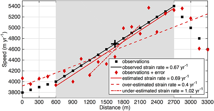
Figure 1. A synthetic surface speed profile representing a fast-flowing tidewater glacier is shown in black and the speed profile plus random errors (±300 m year⁻¹) are shown in red. The SCL is prescribed as 2100 m, which is reasonable for fast-flowing glaciers that are several hundred meters thick (Kamb and Echelmeyer, 1986). The gray shaded rectangle indicates the prescribed SCL, which defines the distance over which the strain rate should be calculated for the pixel marked by the black “+.” The solid, dashed, and dashed-dotted lines display estimated strain rates (i.e., longitudinal speed gradients) for the true, over-estimated, and under-estimated SCLs, respectively.

Theory suggests that the SCL varies as a function of glacier geometry (i.e., thickness and width), the difference between the bulk (i.e., vertically-averaged) effective viscosity and the effective viscosity of basal ice, and the exponent of the glacier flow law that relates stresses and strain rates (Kamb and Echelmeyer, 1986). Accordingly, we expect maximum SCLs in the interior of polar ice sheets (~4–10 ice thicknesses) and much shorter SCLs for temperate alpine glaciers (~1–3 ice thicknesses; Kamb and Echelmeyer, 1986). Early SCL approximations (e.g., Kamb and Echelmeyer, 1986) assumed equal longitudinal and shear effective viscosities, allowing SCL estimations from glacier geometry. In practice, most force balance analyses assume that the SCL can be approximated as a function of the ice thickness. However, methods relating SCL to ice thickness vary widely among analyses. For example, Kavanaugh and Cuffey (2009) estimated SCL scaling factors by relating the ice thickness to the length of the along-flow smoothing window that produces the best match between observed surface speeds and inferred basal speeds. In contrast, O'Neel et al. (2005) estimate the SCL as the length of the isotropic smoothing window required to minimize spurious (i.e., negative) values of basal drag while maintaining the characteristic out-of-phase relationship between the gravitational driving stress and longitudinal stress gradients.

In this paper we present a rigorous, automated method for estimating the SCL from high-resolution surface velocity and elevation observations. Our empirical approach to estimate the SCL utilizes the depth-integrated force balance equations, and therefore requires that bed elevation estimates have similar spatial resolution and coverage as the surface observations. Additionally, ice flow must be dominated by basal sliding (i.e., plug flow conditions). These requirements have so far restricted the extraction of accurate SCL estimates and associated force balance applications to a small sample of marine-terminating glaciers with well-constrained bed elevations. The recent development of mass-conserving bed elevation maps for Greenland (BedMachine Greenland; Morlighem et al., 2014), portions of Antarctica (e.g., Holt et al., 2006; Vaughan et al., 2006), and marine-terminating glaciers outside of the major ice sheets (e.g., McNabb et al., 2012) has, however, created the potential to perform high-resolution force balance analyses for a broad spectrum of glaciers. We focus here on data from Helheim Glacier, a well-studied outlet glacier in SE Greenland, to illustrate our method. The versatility of our empirical SCL estimation method is demonstrated through an additional application to Columbia Glacier, Alaska. Both glaciers have been the subject of extensive study over the last several decades and have observational records of comparable spatial and temporal resolution.

Data and Methods

Our goal is to develop a method for estimating the SCL from the observational datasets required for both force balance analyses and numerical ice flow modeling. These datasets consist of maps of bed and surface elevation, as well as surface velocity, all with comparable spatial resolution. Although the Kamb and Echelmeyer (1986, Equation 32) theory provides the means to directly estimate the SCL from a comprehensive suite of observational data, the effective ice viscosity required to accurately estimate the SCL from theory is largely unknown for fast-flowing glaciers. Therefore, in the absence of a priori SCL estimates, we take a two-step approach to estimate the SCL: (1) solve the force balance equations across adjacent grid cells (i.e., compute the local, over-sampled force balance), then (2) estimate the SCL from the local, over-sampled stress fields themselves.

A brief overview of the force balance method is presented below, followed by a description of the SCL estimation approach. We refer the reader to van der Veen (2013, Section 11.2) for a more detailed description of the force balance method.

Force Balance Method

The gravitational force driving the down-slope flow of ice is balanced by resistive stress generated by frictional forces at the basal and lateral margins and by longitudinal and lateral stress gradients. Thus, where ice flow is dominated by basal sliding rather than internal deformation, the force balance over a vertical column of ice is calculated as

$\begin{array}{rc}{\tau }_{\text{dx}}={\tau }_{\text{bx}}-\frac{\partial }{\partial \text{y}}\left(\text{H}{\text{R}}_{\text{xy}}\right)-\frac{\partial }{\partial \text{x}}\left(\text{H}{\text{R}}_{\text{xx}}\right),& (1)\end{array}$

$\begin{array}{rc}{\tau }_{\text{dy}}={\tau }_{\text{by}}-\frac{\partial }{\partial \text{x}}\left(\text{H}{\text{R}}_{\text{xy}}\right)-\frac{\partial }{\partial \text{y}}\left(\text{H}{\text{R}}_{\text{yy}}\right).& (2)\end{array}$

Subscripts x and y indicate the along- and across-flow directions, τ_d is the gravitational driving stress, τ_b is the basal resistance, H is the ice thickness, and R is the tensile or compressional (subscripts xx and yy) and shear (subscript xy) resistive stresses. To solve (Equations 1, 2), gradients in surface elevation (i.e., surface slope), surface velocity (i.e., strain rates), and depth-integrated resistive stresses must be calculated. To minimize bias that can be introduced by random errors or by the truncation of the averaging window near the glacier margins, we take a hybrid approach of the force balance method and the control method (MacAyeal, 1992) and calculate gradients in elevation, speed, and resistive stresses using a linear regression across the averaging window (van der Veen, 2013), such as illustrated for the calculation of strain rates in Figure 1. The gravitational driving stress is calculated using an ice density of 917 kg m⁻³. Depth-integrated resistive stresses are estimated from surface strain rates using Glen's flow law (Hooke, 2005, p. 66) with an exponent of n = 3. Basal drag is estimated as the residual that satisfies the force balance equalities.

Stress-Coupling Length Estimation

The stress coupling length in a spring under tension can be considered to be the wavelength of the displaced spring coils. To visualize this concept, imagine a spring, not under tension, anchored at both ends, resting on a high-friction surface. If you gently pull on one of the coils, only a few coils will be displaced because the force exerted through tension is rapidly dissipated with distance from the tensional source due to friction. As you increase the stress exerted on the spring (i.e., pull more forcefully), more coils begin to stretch and the length over which the coils are displaced increases. You are not directly pulling on the interior coils, but they unfurl because the force is distributed along a portion of the spring. The distance that the force exerted by your hand is transferred along the spring (i.e., SCL) is the distance over which the coils are displaced (i.e., the wavelength). The displacement of the coils themselves reveals the SCL. By analogy, the periodicity of oscillations in resistive stresses can be used as a proxy for the SCL in glaciers.

Stress coupling is more complicated for glaciers, however, due to the relationship between stress, strain rates, and effective viscosity. The differences in effective viscosity of ice undergoing tensile and shear stresses further complicate matters. As shown by Kamb and Echelmeyer (1986) and confirmed by Kavanaugh and Cuffey (2009), the SCL varies in the along-flow direction with the tensile and compressional (i.e., longitudinal) stresses and basal shear stress (i.e., basal drag). Following this precedent, we solve the force balance equations (Equations 1, 2) using a centered-differences approach and calculate the along-flow resistive stress as the sum of the local longitudinal stresses and basal drag. Stresses calculated in this manner are over-sampled, meaning the large-scale oscillations in longitudinal and basal stresses that reflect stress coupling will be superimposed on high-frequency stress anomalies introduced in part by random errors in the observational datasets. To ensure that potential spatial variations in the SCL are preserved, we extract the periodicity of the large-scale oscillations in stresses from multiple flow-following profiles (i.e., flowlines). The optimal number of profiles is somewhat subjective, but should be selected based on the glacier width and spatial resolution of the observational data. The number of profiles should also take into account considerable across-flow variations in thickness and/or rheology, such as those expected for complex glacier systems (i.e., glaciers with multiple tributaries), which may result in spatial variations in the SCL.

We use an automated, signal processing approach to estimate the SCL from the stress profiles. To assess whether this automated approach sufficiently resolves potential spatial variations in the SCL, we compare SCLs obtained using our automated approach to SCLs that are manually extracted from the stress profiles. For the automated estimates, we pre-process local resistive stress profiles for each observation date by normalizing them to vary about zero. The detrended profiles are tapered using a Hann (raised cosine) window that minimizes endpoint discontinuities to prevent spectral leakage. Resistive stress oscillations are then identified using periodograms constructed from the pre-processed profiles.

Assuming that the SCL does not vary considerably along each profile, the periodograms should return peaks in spectral power for the periods that correspond to the SCLs. In order to resolve the SCL in this manner, however, we must account for the exponential decrease in power with increased period length that is expected for spatially correlated data (i.e., a red noise distribution (Bartlett, 1955); power weighted toward lower frequencies). For each periodogram, we approximate the underlying red noise power spectrum using a linear regression of the logarithm of the periodogram (Vaughan, 2005) and calculate the residual power. We then estimate the SCL as the dominant periodicity (i.e., highest residual power) that falls within the analytically-derived minimum SCL of 1H (Bahr et al., 1994) and the theoretical maximum SCL of 10H for polar ice (Kamb and Echelmeyer, 1986), where H is the average ice thickness for the profile. Finally, we average stress profiles for as many time intervals as possible over a relatively quiescent period of dynamic change. Temporal averaging of the stress profiles has a similar effect on the SCL estimates as periodogram stacking because it minimizes observational errors, which increases the signal-to-noise ratio in the periodograms. The averaging also minimizes aliasing effects caused by short-term changes in ice flow and surface accumulation and/or ablation and reduces the effect of spatial data gaps, improving the accuracy of our automated SCL estimates.

Uncertainties in SCL Estimates

The surface speed and ice thickness observations used to estimate SCL benefit from higher spatial resolution and lower uncertainties than datasets that were available a decade ago. However, inversion of surface observations to estimate basal drag remains mathematically ill-posed (Bahr et al., 2014), leading to large uncertainties in the over-sampled stress estimates that we use to estimate the SCL. Several forms of observational errors exist, including: spatial and temporal variation in ice motion, and random errors associated with measuring ice motion as well as spatially systematic but transient errors (i.e., aliasing errors). Below we discuss each source of observational uncertainty, emphasizing methods to minimize their impact on SCL estimates.

Ice motion and surface elevation data are subject to a diffusive smoothing algorithm (Perona and Malik, 1990), which increases spatial correlation between adjacent pixels and reduces random error while preserving the sharp gradients in ice speed observed near the lateral margins and the calving front (Martin, Pers. Commun., 2014). Remaining random errors in the observational data are further minimized through temporal averaging of the stress profiles. Diffusive smoothing of the velocity maps and temporal averaging of the stress profiles also minimizes the impacts of spatial and temporal aliasing errors that can be introduced due to variability in motion and ice thickness over tidal to seasonal time scales, as well as by in-filling of raster data gaps.

Applications and Discussion

In practice, comprehensive determination of SCL using our empirical approach applied to contiguous flow-following profiles spanning entire glacierized catchments is computationally expensive. As a result, we choose to estimate the SCL for relatively sparse (~0.5–1 km separation) profile arrays then, following theory and convention, use these empirical SCL estimates to parameterize the SCL over the entire glacierized catchment as a function of ice thickness. The empirical scaling relationship between the SCL and thickness from our sparse profiles allows us to estimate the SCL for each pixel in the domain. We apply our SCL estimation approach and compute empirical thickness-scaling relationships for two well-studied fast-flowing tidewater glaciers: Helheim Glacier, SE Greenland and Columbia Glacier, Alaska, USA. Use of the standardized approach developed here will enable direct inter-comparisons of the force balance method at the two sites. In the examples presented below, we demonstrate the ability of our empirical SCL estimation approach to (1) resolve both intra- and inter-glacier variations in the SCL and (2) illustrate the sensitivity of SCL estimates and thickness-scaling parameterizations to observational uncertainties.

Observational Data

Surface elevations were extracted from stereo images collected by the Advanced Spaceborne Thermal Emission and Reflection Radiometer (ASTER) and WorldView-1 and -2 satellites. The 30 m-resolution ASTER digital elevation models (DEMs) are available from the NASA Earth Observing System Data and Information System (NASA EOSDIS; http://reverb.echo.nasa.gov). High-resolution (~1.5 m) WorldView DEMs were produced following the methods described in Shean et al. (2016). A total of 18 DEMs were compiled for each glacier (Table 1). The Helheim DEMs span the 2010–2014 period, with most (16/18) observations acquired from May-August of each year. Although DEMs of Columbia Glacier are also available over the entire 2010–2014 period, we restricted our DEM database to the 2012–2013 period when the glacier surface elevations remained fairly constant (i.e., within ±10 m of the mean for the same period). Random errors in DEM-derived surface elevations were estimated as ~7 m for the ASTER products (Stearns and Hamilton, 2007) and ~3 m for WorldView DEMs (Enderlin and Hamilton, 2014). Systematic biases in DEM-derived elevations were minimized through vertical co-registration of overlapping DEMs using exposed bedrock elevations (Nuth and Kääb, 2011). Horizontal uncertainties are comparable to the DEM pixel size (Stearns and Hamilton, 2007).

TABLE 1

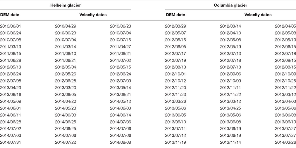
Table 1. Dates of digital elevation models (DEMs) and velocities for Helheim Glacier, SE Greenland, and Columbia Glacier, Alaska, USA, that are used for our SCL estimates.

We calculated ice thickness as the difference between ice surface and bed elevations. Bed elevations for Helheim Glacier were taken from the 150 m-resolution BedMachine Greenland dataset (Morlighem et al., 2014; http://nsidc.org/data/docs/daac/icebridge/idbmg4/index.html), which is based on mass conservation and constrained by ice-penetrating radar observations. Uncertainties increase with distance from radar profiles, and were estimated as an average of ~50 m over the glacier's fast-flowing trunk (Morlighem et al., 2014). Columbia bed elevations were estimated using the same mass conservation algorithm and constrained using a subset of ice-penetrating radar observations from Rignot et al. (2013) that were manually checked for errors introduced by off-nadir reflections using a surface clutter prediction algorithm (Holt et al., 2006). Only bed echoes verified by this algorithm were retained for our study. Using these radar data, we found that the glacier is ~50–250 m thinner along its fast-flowing core and ~50–150 m thicker along its lateral margins than previously estimated (McNabb et al., 2012). As with Helheim, the uncertainties in the bed elevations increase with distance from the radar profiles, with an average vertical uncertainty of ~15 m. The filtered radar observations and bed elevation map for Columbia Glacier can be accessed on the Maine DataVerse Network (MDVN; http://dataverse.acg.maine.edu/dvn/dv/eep).

Surface velocities for Helheim Glacier were extracted from the NASA Making Earth System Data Records for Use in Research Environments (MEaSUREs) product (NSIDC; http://nsidc.org/data/nsidc-0481/) produced using TerraSAR-X interferometric synthetic aperture radar (InSAR) measurements. The velocity product is posted at a 150 m spatial resolution. Columbia Glacier velocities were calculated using the same approach and have a spatial resolution of 100 m. Random errors were estimated from local variations in ice velocity and systematic errors were estimated as 3% of the speed (Joughin et al., 2010). Velocity dates are listed in Table 1.

To standardize the datasets and referencing systems, we down-sampled the co-registered DEMs from their native resolution and interpolated the bed elevation grids to the 150 m-resolution InSAR velocity grids using a linear distance-weighted approach similar to O'Neel et al. (2005). DEM data gaps were filled using an iterative nearest neighbor algorithm (Garcia, 2010). Velocities corresponding to each DEM were estimated by averaging the two InSAR velocity maps closest in time (typically within ~2 weeks) to the DEM acquisition date, which minimizes the impact of short-term (hourly to monthly) variability in ice dynamics. After determining SCLs, the force balance equations (Equations 1, 2) were solved using a temperature-dependent viscosity parameter of B = 1.02 × 10⁸ Pa s^1/3 corresponding to an average ice temperature of −5°C for Helheim Glacier (Nick et al., 2009) and a viscosity parameter appropriate for temperate ice (B = 7.47 × 10⁷ Pa s^1/3) for Columbia Glacier (Nick et al., 2007).

Example Application: Helheim Glacier

The domain and input data for SCL estimates at Helheim Glacier in SE Greenland are shown in Figure 2. At Helheim, we extracted ice thickness and resistive stress along five flowlines spanning the main trunk and major tributaries (Figure 2, dashed lines). For Figure 2 and for our SCL thickness-scaling parameterization, we use the median ice thickness from the 18 DEMs compiled for the 2010–2014 period. We use the median thickness, not the mean, to minimize biases in the derived thickness-scaling parameterization introduced by blunders in the DEMs.

FIGURE 2

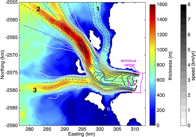
Figure 2. Median thickness (colors) and surface speed (gray contours) for Helheim Glacier. Major tributaries are numbered. Dashed black lines indicate the tributary and trunk flowlines from which stress and thickness profiles are extracted. The range of TSX-derived terminus positions for the 2010–2014 period is outlined in pink. Speed contours are truncated at the average terminus position over the study period. Coordinates are provided in the Greenland polar stereographic projection.

Thickness and resistive stress profiles from the central flowline of Helheim Glacier are shown in Figures 3A,B, highlighting how temporal averaging preserves periodicity while reducing high-frequency noise in the stress profiles and resulting power spectra (Figure 3C). Temporal averaging also ensures that variability in the spatial extent of the datasets do not bias the periodogram-derived SCL estimates. The large variations in automated SCL estimates (Figure 4A) suggest that the SCL varies considerably within the glacier catchment. The presence of along-flow variations in the SCL is verified through manual inspection of the stress profiles and the derived periodograms. The distance between local resistive stress maxima are manually extracted from the stress profiles, as demonstrated in Figure 3A, and used as a proxy for along-flow changes in the SCL. Using this approach, we obtain manual SCL estimates that can be clustered into two SCLs: 2321 ± 43 m and 3524 ± 430 m. Manual inspection of the associated periodograms (Figure 3C) reveals primary and secondary significant peaks (i.e., positive residual power) at ~3800 and ~2000 m, respectively, that are in good agreement with the manual SCL estimates.

FIGURE 3

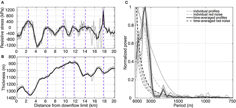
Figure 3. (A) Along-flow resistive stress profiles, (B) thickness profiles, and (C) normalized periodograms from the main tributary (trib. 2) for Helheim Glacier (Figure 2). Thin gray lines distinguish profiles for individual observation dates and thick black lines show time-averaged profiles. The vertical dashed purple lines in (A,B) mark the manually-identified local stress maxima. Solid lines in (C) show the normalized spectral power (i.e., fractional power) for the along-flow resistive stress profiles in (A) and dashed lines show the modeled underlying red noise power spectra.

FIGURE 4

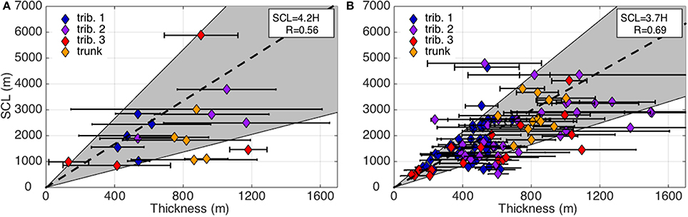
Figure 4. Automatic SCL estimates plotted against the average ice thickness for Helheim Glacier. (A) The SCL is estimated for each 20–40 km-long median resistive stress profile using an automated approach and the thickness is estimated as the average over the entire profile length. (B) SCL estimates and average ice thickness for the segmented profiles. The horizontal error bars in both panels indicate the range in ice thickness over the portion of the profile for which the SCL is estimated. The dashed lines show the time-averaged SCL:H ratios, with slopes and correlation coefficients given in the top right corner of each panel. Gray shading defines the ±1σ envelope, where σ is the standard deviation in SCL:H ratios (σ = 2.5 and σ = 1.7 for (A,B), respectively).

Although the along-flow variations in the SCL can be manually extracted from the resistive stress profiles, random errors in the observational data can obscure the local stress maxima, leading to subjective SCL estimates. To capture along-flow variations in the SCL, we instead use a moving window to segment the stress profiles and extract the SCL from each segment using our automated, periodogram-based approach. The segment length and sampling interval is chosen to minimize aliasing of SCL variability: the length of the moving window is slightly (10%) longer than 2 × SCL_mean, where SCL_mean is the mean SCL estimate for the profile,and there is 50% overlap between window segments. Given the theoretical and observed correlation between SCL and the ice thickness (Figure 4A), we estimate SCL_mean as the product of the mean profile thickness and the mean SCL:H ratio for the full-length time-averaged profiles (Figure 4A; SCL = 4.2H). SCL_mean values range from ~700 m to ~5.3 km, corresponding to segment lengths ranging from ~1.5 to ~11.7 km. The segmented automated approach yields an average SCL:H ratio for all segments of 3.7 (Figure 4B), which is in good agreement with the manually-derived average of 3.8. Profile segmentation also reduces variability in the SCL:H ratio and increases the strength of the correlation between the SCL and ice thickness: σ = 2.5 and R = 0.56 for the time-averaged profiles and σ = 1.7 and R = 0.69 for the segmented profiles, where σ is the standard deviation in the SCL:H ratio. Thus, in-line with theory and convention, we use the automated SCL estimates extracted from the segmented profiles to construct a thickness-scaling parameterization that allows us to extrapolate the SCL over the entire glacier domain.

In order to analyze spatial and temporal variations in the force balance terms, Equations (1, 2) must be solved over the area spanning the along- and across-flow SCL. For each pixel, the stress-coupling area, or SCA, is defined as the centered rectangular area spanning the SCL in the along-flow and transverse directions. Following convention, we first calculate gradients in surface elevation, velocity, and resistive stresses in the x- and y- directions as the average slope of a least-squares regression spanning the SCA. These values allow us to solve Equations (1, 2), then rotate the stresses into flow-following coordinates. Estimated uncertainties and root mean square errors (RMSEs) for each term are derived using a similar approach as van der Veen (2013, Section 3.6). We assume that the slope of the regression is approximately equal to the mean inter-pixel gradient and estimate random errors in the x and y directions as

$\begin{array}{l}{\sigma }_{\frac{\partial }{\partial \text{x}}\left(\text{H}{\text{R}}_{\text{ij}}\right)}=\sqrt{{{\displaystyle \sum }}_{\text{k}=1}^{\text{n}-1}\frac{{\sigma }_{\text{H}{\text{R}}_{\text{ij}}\left(\text{k}+1\right)}^2+{\sigma }_{\text{H}{\text{R}}_{\text{ij}}\left(\text{k}\right)}^2}{\partial {\text{x}}^2}}\\ \approx \frac{1}{|\partial \text{x}|}\sqrt{\frac{2}{\text{n}-1}{{\displaystyle \sum }}_{\text{k}=1}^{\text{n}}{\sigma }_{\text{H}{\text{R}}_{\text{ij}}\left(\text{k}\right)}^2},\hfill & (3)\end{array}$

where i,j = x,y and n is the length of the SCL (in pixels). Errors are calculated using Equation (3), with x = y, for the y-direction. To estimate the total error, an additional 3% error is added to the depth-integrated strain rates to account for non-random uncertainties in the ice flow velocities. Force balance estimates obtained using our empirical SCL parameterization are demonstrated for Helheim Glacier in Figure 5. Following convention, the gravitational driving stress (Figure 5A) is positive along-flow and the resistive stresses are positive against flow (Figures 5B–D). Uncertainties associated with each force balance term are shown in Figures 5E–H. Figures 5I–K show the normalized RMSEs of the linear least-squares regressions (i.e., RMSE/RMSE_max), which provide a means to identify regions where under-estimation of the SCL would lead to large errors in force balance calculations: higher (lower) normalized RMSEs correspond to more (less) variability in local stresses over the SCA.

FIGURE 5

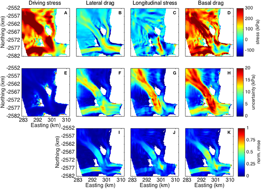
Figure 5. (A–D) Stress, (E–H) uncertainty estimates, and (I–K) normalized (i.e., fractional) root mean square error calculated for Helheim Glacier on June 6, 2010. The different stress components are arranged by column: 1-gravitational driving stress, 2-lateral drag, 3-longitudinal stress, 4-basal drag. The color bars at the end of each row apply to all panels in that row.

As expected, the gravitational driving stress is largest along the glacier's dominant tributary (tributary 2) where the ice thickness reaches a maximum of ~1600 m and the along-flow surface slope is ~0.05 m/m. Driving stress approaches zero along the main trunk where the surface slope approaches zero and the ice nears flotation (De Juan et al., 2010; Figure 5A). The strong across-flow gradients in speed near the glacier's lateral margins lead to narrow zones where lateral stresses pull the slow-flowing margins in the direction of ice flow (Figure 5B, dark blue). Inward of the extensional shear margins, we observe wide bands of high lateral shear (>100 kPa). Alternating bands of longitudinal extension and compression out-of-phase with oscillations in the gravitational driving stress are evident for all three tributaries but are most pronounced at the confluence of the tributaries where the ice is advected over a bedrock or till ridge that rises ~200 m from the surrounding bed (Figure 5C) and the ice originating from the dominant tributary reaches its thickness minimum (Figure 2). Basal drag is generally highest near the lateral margins and increases inland from approximately zero at the down-flow limit (Figure 5D). A comparison of our basal drag estimates with the basal drag parameterization used to simulate the mid-2000s changes in Helheim dynamics (Nick et al., 2009) provides a means to assess the accuracy of our force balance results. We find that the difference between our width-averaged basal drag estimates and the basal drag parameterization in the 1-dimensional (i.e., width-averaged) ice flow model of Nick et al. (2009) is within the estimated uncertainty of ~20 kPa, indicating that the force balance method yields reasonable estimates of basal drag for Helheim Glacier when calculated over the appropriate spatial scales.

Isolated patches of negative (>−50 kPa) basal drag are observed in several locations along the glacier trunk. Negative based drag (i.e., friction at the ice-bed interface pushing the glacier toward the terminus) is physically untenable, and can be attributed to observational errors or failure of the force balance method to realistically capture the physics of ice flow. Although, comparable in magnitude to the stress uncertainty introduced by observational errors, the spatial distribution of these patches of negative basal drag cannot be explained by random errors in observational data. Temporal aliasing introduced by the use of the unweighted average InSAR velocities to approximate surface velocities on the DEM acquisition dates may result in over- or under-estimation of basal drag. However, over the short time periods separating the repeat observations used here, it is unlikely that temporal variations in velocity can fully explain the presence of negative basal drag along the trunk. We instead attribute the region of negative basal drag spanning the trunk at easting ~301 km to failure in the depth-integrated force balance equations to capture the viscous and brittle deformation that likely occurs as the ice is advected through the relatively deep trough and over the ~200 m-tall bedrock ridge at the confluence of the tributaries. Within one SCL of the end of the glacier domain, prominent regions of negative basal drag emerge. These regions of negative basal drag are not due either to observational errors or failure in the force balance method, but can be explained by the truncation of the mass conservation-based bed elevation map. The bed elevation map was constructed using surface elevation observations acquired when the terminus was retracted relative to its present location, causing truncation of our depth-integrated stress estimates inland of the true terminus position. The hydrostatic imbalance between the glacier terminus and fjord water leads to longitudinal extension immediately inland of the terminus. Therefore, truncation of our stress estimates inland of the terminus leads to the omission of this zone of longitudinal extension and over-estimation of longitudinal resistance at the terminal end of the truncated domain. Despite these limitations, the relatively low uncertainty and high spatial resolution of the depth-integrated driving and resistive stresses shown in Figure 5 suggest that our empirical SCL parameterization will be beneficial for studies aimed at resolving the controls of changes in glacier dynamics. Notably, although our SCL parameterization is developed using time-averaged local stresses, the parameterization can be applied to temporally-evolving force balance analyses to investigate changes in driving and resistive stresses in response to environmental perturbations.

Example Application: Columbia Glacier

The versatility of our empirical SCL estimation approach is demonstrated using observational data from a temperate marine-terminating mountain glacier, which according to theory, may have a smaller thickness-scaling ratio than estimated for the larger and colder Helheim Glacier (Kamb and Echelmeyer, 1986). We selected Columbia Glacier, Alaska over an additional Greenland outlet glacier, for several reasons: it (1) is considerably smaller (~3 km-wide and <700 m-thick) and less viscous than Helheim Glacier, (2) has a detailed observational record of surface elevations and velocities and a bed elevation map of comparable spatial resolution to Helheim (Figure 6), and (3) has been the target of previous SCL and force balance analyses (e.g., Walters, 1989; van der Veen and Whillans, 1993; O'Neel et al., 2005) to which we can compare our analyses.

FIGURE 6

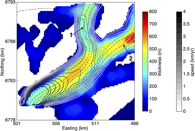
Figure 6. Median thickness (color shading) and surface speed (gray contours) estimated from digital elevation models and InSAR velocities acquired for Columbia Glacier over the 2012–2013 period. Major tributaries are numbered. Ice flows through tributaries 1 and 2 toward the terminus in the southwest, where the thickness and speed domain ends. Dashed black lines indicate the tributary and trunk flowlines from which stress and thickness profiles are extracted. Coordinates are in UTM Zone 6N.

Given the sparse spatial coverage of ice-penetrating radar observations (Rignot et al., 2013), the spatial domain over which reliable thickness (and stress) estimates can be obtained is quite limited relative to the Helheim Glacier datasets. Thus, in order to ensure that our stress profiles are sufficiently long to accurately estimate the SCL using our automated approach (i.e., long periods are not truncated), we refrain from extracting separate stress profiles for the trunk and tributaries and instead extend the tributary profiles into the glacier trunk (Figure 6). For the full profiles, we obtain an average SCL of ~1400 m, which corresponds to a SCL:H ratio of 5.6 (Figure 7A). As with Helheim, we segment the resistive stress profiles in order to resolve potential spatial variations in SCL corresponding with along-flow changes in ice thickness. We find an average SCL of ~1150 m, a moderate strength relationship between variations in the SCL and ice thickness (R = 0.54), and a mean SCL:H ratio of 4.3 (Figure 7B).

FIGURE 7

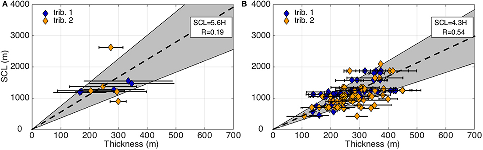
Figure 7. Automatic, time-averaged SCL estimates plotted against the average ice thickness for Columbia Glacier. (A) The SCL is estimated for each 15–20 km-long median resistive stress profile using an automated approach, and the thickness is estimated as the average over the entire profile length. (B) SCL estimates and average ice thickness for the segmented profiles. The horizontal error bars in both panels indicate the range in ice thickness over the portion of the profile for which the SCL is estimated. The dashed lines show the time-averaged SCL:H ratios, with slopes and correlation coefficients given in the top right corner of each panel. Gray shading defines the ±1σ envelope, where σ is the standard deviation.

We attribute the uniformity of the Columbia SCL that is apparent in Figure 7 not to failure of our empirical SCL estimation approach but rather to strong stress coupling between the lateral margins and fast-flowing core. To assess the importance of transverse stress-coupling for Columbia's trunk, we derive independent estimates for the transverse SCL from profiles of lateral shear stresses, extracted perpendicular to the centerline flow direction at 600 m increments along-flow. Using this approach, we obtain long transverse SCL estimates (1610 ± 600 m) that indicate strong stress coupling across the glacier trunk. Thus, it is not surprising that the SCL extracted from the lateral margins (down-flow reaches of tributary 2 in Figure 6), where the ice thickness is <300 m, is indistinguishable from the centerline SCL.

Our SCL estimates for Columbia Glacier are in good agreement with the independent SCL estimate of 1200 m in (O'Neel et al., 2005). Taking into account the relatively flat cross-sectional shape of Columbia Glacier and the non-linear increase in the theoretical SCL:H ratio with flattening of glacial cross-sectional area (see Kamb and Echelmeyer, 1986; Figure 5), our SCL:H ratio of 4.3 ± 1.2 is also in good agreement with theory. Thus, based on the results of the example applications presented here, we are confident that our empirical approach for estimating the SCL can be successfully applied to glaciers encompassing a wide range of geometries and ice rheologies.

Conclusions

Using high-resolution observations of surface and bed elevations and surface velocities for two marine-terminating glaciers, we demonstrate an empirical approach for estimating the SCL that determines the spatial resolution of force balance analyses. We solve for the SCL as the dominant period of oscillations in the sum of longitudinal stresses and basal drag in the along-flow direction. In line with Kavanaugh and Cuffey (2009), we find that the SCL can be approximated as a linear function of the ice thickness for Helheim Glacier. Although the strength of the correlation is slightly weaker for Columbia Glacier, our empirical SCL estimates are in good agreement with previous independent estimates and theory, indicating that the method can be applied to a range of glacier geometries and ice rheologies.

The use of a standardized method for estimating the SCL allows direct comparison of stress redistribution time series between glaciers, which is critical for improving the current understanding of glacier dynamics. Thus, we suggest that studies of the dynamic redistribution of driving and resistive stresses following a change in environmental forcing adopt a similar empirical approach to estimating the SCL. The code developed for our empirical approach is available on the MDVN (http://dataverse.acg.maine.edu/dvn/dv/eep). By using high-resolution datasets to simultaneously calculate the glacier force balance and the SCL, such as illustrated here, force balance analyses have the potential to improve the current understanding of glacier dynamics in a rapidly changing climate.

Author Contributions

EE and SO conceived the initial project idea. EE developed the methodology, generated the digital elevation models, compiled the observational datasets, applied the method to the Helheim and Columbia observations, and wrote the manuscript. GH, SO, and TB provided feedback on the method and revised the manuscript. JH revised bed picks from the Columbia Glacier radar dataset and MM used the revised picks to constrain the mass conservation-derived bed elevation map. JH and MM also contributed to final manuscript revisions.

Conflict of Interest Statement

The authors declare that the research was conducted in the absence of any commercial or financial relationships that could be construed as a potential conflict of interest.

Acknowledgments

This work was supported by NASA award NNX14AH83G to EE, SO, and GH. WorldView images were distributed by the Polar Geospatial Center at the University of Minnesota (http://www.pgs.umn.edu/imagery/satellite) as part of an agreement between the US National Science Foundation and the US National Geospatial Intelligence Agency Commercial Imagery Program. DEMs were generated from WorldView images using supercomputing resources provided by the University of Maine Advanced Computing Group. The DEMs, Columbia bed elevation map and filtered radar profiles, and Matlab code used to extract the SCL estimates are archived on the Maine DataVerse Network (http://dataverse.acg.maine.edu/dvn/dv/eep). TSX terminus positions for Helheim Glacier were provided by Twila Moon. We thank David Bahr and Jason Amundson for providing feedback on the methods and Evan Burgess for his help with the initial stages of data processing. The findings and conclusions in this article are those of the author(s) and do not necessarily represent the views of any government agencies.

References

Armstrong, W. H., Anderson, R. S., Allen, J., and Rajaram, H. (2016). Modeling the WorldView-derived season velocity evolution of Kennicott Glacier, Alaska. J. Glaciol. 62, 763–777. doi: 10.1017/jog.2016.66

CrossRef Full Text | Google Scholar

Bahr, D. B., Pfeffer, W. T., and Kaser, G. (2014). Glacier volume estimation as an ill-posed inversion. J. Glaciol. 60, 922–934. doi: 10.3189/2014JoG14J062

CrossRef Full Text | Google Scholar

Bahr, D. B., Pfeffer, W. T., and Meier, M. F. (1994). Theoretical limitations to englacial velocity calculations. J. Glaciol. 40, 509–518.

Google Scholar

Bartlett, M. S. (1955). An Introduction to Stochastic Processes. Cambridge: Cambridge University Press.

Google Scholar

De Juan, J., Elósegui, P., Nettles, M., Larsen, T. B., Davis, J. L., Hamilton, G. S., et al. (2010). Sudden increase in tidal response linked to calving and acceleration at a large Greenland outlet glacier. Geophys. Res. Lett. 37, L12501. doi: 10.1029/2010GL043289

CrossRef Full Text | Google Scholar

Enderlin, E. M., and Hamilton, G. S. (2014). Estimates of iceberg submarine melting from high-resolution digital elevation models: application to Sermilik Fjord, East Greenland. J. Glaciol. 60, 1084–1092. doi: 10.3189/2014JoG14J085

CrossRef Full Text | Google Scholar

Enderlin, E. M., Howat, I. M., Jeong, S., Noh, M. J., van Angelen, J. H., and van den Broeke, M. R. (2014). An improved mass budget for the Greenland ice sheet. Geophys. Res. Lett. 41, 866–872. doi: 10.1002/2013GL059010

CrossRef Full Text | Google Scholar

Garcia, D. (2010). Robust smoothing of gridded data in one and higher dimensions with missing values. Comput. Stat. Data Anal. 54, 1167–1178. doi: 10.1016/j.csda.2009.09.020

PubMed Abstract | CrossRef Full Text | Google Scholar

Holt, J. W., Blankenship, D. D., Morse, D. L., Young, D. A., Peters, M. E., Kempf, S. D., et al. (2006). New boundary conditions for the West Antarctic Ice Sheet: subglacial topography of the Thwaites and Smith glacier catchments. Geophys. Res. Lett. 33, L09502. doi: 10.1029/2005GL025561

CrossRef Full Text | Google Scholar

Hooke, R. L. (2005). Principles of Glacier Mechanics, 2nd Edn. Cambridge: Cambridge University Press.

Google Scholar

Joughin, I., Smith, B. E., Howat, I. M., Scambos, T., and Moon, T. (2010). Greenland flow variability from ice-sheet-wide velocity mapping. J. Glaciol. 56, 415–430. doi: 10.3189/002214310792447734

CrossRef Full Text | Google Scholar

Kamb, B., and Echelmeyer, K. A. (1986). Stress-gradient coupling in glacier flow: I. Longitudinal averaging of the influence of ice thickness and surface slope. J. Glaciol. 32, 267–284.

Kavanaugh, J. L., and Cuffey, K. M. (2009). Dynamics and mass balance of Taylor Glacier, Antarctica: 2. force balance and longitudinal coupling. J. Geophys. Res. 114, F04011. doi: 10.1029/2009jf001329

CrossRef Full Text | Google Scholar

MacAyeal, D. R. (1992). The basal stress distribution of Ice Stream E, Antarctica, inferred by control methods. J. Geophys. Res. 97, 595–603. doi: 10.1029/91JB02454

CrossRef Full Text | Google Scholar

Maxwell, D., Truffer, M., Avdonin, S., and Stuefer, M. (2008). An iterative scheme for determining glacier velocities and stresses. J. Glaciol. 54, 888–898. doi: 10.3189/002214308787779889

CrossRef Full Text | Google Scholar

McNabb, R. W., Hock, R., O'Neel, S., Rasmussen, L. A., Ahn, Y., Braun, M., et al. (2012). Using surface velocities to calculate ice thickness and bed topography: a case study at Columbia Glacier, Alaska, USA. J. Glaciol. 58, 1151–1164. doi: 10.3189/2012JoG11J249

CrossRef Full Text | Google Scholar

Morlighem, M., Rignot, E., Mouginot, J., Seroussi, H., and Larour, E. (2014). Deeply incised submarine glacial valleys beneath the Greenland ice sheet. Nat. Geosci. 7, 418–422. doi: 10.1038/ngeo2167

CrossRef Full Text | Google Scholar

Nick, F. M., van der Veen, C. J., and Oerlemans, J. (2007). Controls on advance of tidewater glaciers: results from numerical modeling applied to Columbia Glacier. J. Geophys. Res. 112, F03S24. doi: 10.1029/2006JF000551

CrossRef Full Text | Google Scholar

Nick, F. M., Vieli, A., Howat, I. M., and Joughin, I. (2009). Large-scale changes in Greenland outlet glacier dynamics triggered at the terminus. Nat. Geosci. 2, 110–114. doi: 10.1038/ngeo394

CrossRef Full Text | Google Scholar

Nuth, C., and Kääb, A. (2011). Co-registration and bias corrections of satellite elevation data sets for quantifying glacier thickness change. Cryosphere 5, 271–290. doi: 10.5194/tc-5-271-2011

CrossRef Full Text | Google Scholar

O'Neel, S., Pfeffer, W. T., Krimmel, R., and Meier, M. (2005). Evolving force balance at Columbia Glacier, Alaska, during its rapid retreat. J. Geophys. Res. 110, F03012. doi: 10.1029/2005JF000292

CrossRef Full Text | Google Scholar

Perona, P., and Malik, J. (1990). Scale-space and edge detection using anisotropic diffusion. IEEE Trans. Pattern Anal. Mach. Intell. 12, 629–639. doi: 10.1109/34.56205

CrossRef Full Text | Google Scholar

Rignot, E., Mouginot, J., Larsen, C. F., Gim, Y., and Kirchner, D. (2013). Low-frequency radar sounding of temperate ice masses in Southern Alaska. Geophys. Res. Lett. 40, 5399–5405. doi: 10.1002/2013GL057452

CrossRef Full Text | Google Scholar

Sergienko, O. V., and Hindmarsh, R. C. A. (2013). Regular patterns in frictional resistance of ice-stream beds seen by surface data inversion. Science 342, 1086–1089. doi: 10.1126/science.1243903

PubMed Abstract | CrossRef Full Text | Google Scholar

Shean, D. E., Alexandrov, O., Moratto, Z. M., Smith, B. E., Joughin, I. R., Porter, C., et al. (2016). An automated, open-source pipeline for mass production of digital elevation models (DEMs) from very-high-resolution commercial stereo satellite imagery. ISPRS J. Photogram. Remote Sens. 116, 101–117. doi: 10.1016/j.isprsjprs.2016.03.012

CrossRef Full Text | Google Scholar

Stearns, L. A., and Hamilton, G. S. (2007). Rapid volume loss from two East Greenland outlet glaciers quantified using repeat stereo satellite imagery. Geophys. Res. Lett. 34, L05503. doi: 10.1029/2006GL028982

CrossRef Full Text | Google Scholar

van der Veen, C. J. (2013). Fundamentals of Glacier Dynamics, 2nd Edn. Boca Raton, FL: CRC Press.

Google Scholar

van der Veen, C. J., Stearns, L. A., Johnson, J., and Csatho, B. (2014). Flow dynamics of Byrd Glacier, East Antarctica. J. Glaciol. 60, 1053–1064. doi: 10.3189/2014JoG14J052

CrossRef Full Text | Google Scholar

van der Veen, C. J., and Whillans, I. M. (1989). Force budget. 1. Theory and numerical-methods. J. Glaciol. 35, 53–60. doi: 10.3189/002214389793701581

CrossRef Full Text | Google Scholar

van der Veen, C. J., and Whillans, I. M. (1993). Location of mechanical controls on Columbia Glacier, Alaska, USA, prior to its rapid retreat. Arctic Alpine Res. 25, 99–105. doi: 10.2307/1551545

CrossRef Full Text | Google Scholar

Vaughan, D. G., Corr, H. F. L., Ferraccioli, F., Frearson, N., O'Hare, A., Mach, D., et al. (2006). New boundary conditions for the West Antarctic ice sheet: subglacial topography beneath Pine Island Glacier. Geophys. Res. Lett. 33, L09501. doi: 10.1029/2005GL025588

CrossRef Full Text | Google Scholar

Vaughan, S. (2005). A simple test for periodic signals in red noise. Astron. Astrophys. 431, 391–403. doi: 10.1051/0004-6361:20041453

CrossRef Full Text | Google Scholar

Vieli, A., and Nick, F. M. (2011). Understanding and modelling rapid dynamic changes of tidewater outlet glaciers: issues and implications. Surv. Geophys. 32, 437–458. doi: 10.1007/s10712-011-9132-4

CrossRef Full Text | Google Scholar

Walters, R. A. (1989). Small amplitude, short period variations in the speed of a tidewater glacier in south-central Alaska. Ann. Glaciol. 12, 187–191.

Google Scholar

Whillans, I. M., Chen, Y. H., van der Veen, C. J., and Hughes, T. J. (1989). Force budget. 3. Application to 3-dimensional flow of Byrd Glacier, Antarctica. J. Glaciol. 35, 68–80. doi: 10.3189/002214389793701554

CrossRef Full Text | Google Scholar