Dynamic modeling of the microalgae cultivation phase for energy production in open raceway ponds and flat panel photobioreactors

Introduction

Microalgae are single cell organisms, which can be found in colonies or individual cells. Their most interesting characteristic is the ability of realizing a photosynthetic reaction in a single cell. They are extremely resistant and may grow in many different environments, from fresh water to marine and hyper-saline water (Le et al., 2010; Mata et al., 2010). Microalgae can be seen as an interesting alternative to more typical biomass as a source for biofuels production. Studies on microalgae have been carried out since the 1980s, but in recent years their importance has grown fast: as Chisti (2007) claims, the reason is that microalgae appear to be the only source of biodiesel that has the potential to completely displace fossil diesel. Moreover, compared to other biofuels sources, such as traditional crops and wood, microalgae have several advantages: they grow extremely fast, reaching high areal and volumetric productivities; they do not require arable land; they ask for less freshwater than normal crops, being able to use wastewater; they can directly capture CO₂ released by industries and they overtake the food vs. fuel debate; and their ability to grow in a wide range of conditions, resisting to severe temperatures, pH, and salinity (NREL, 0000), makes them even more attractive.

In 1978, the National Renewable Energy Laboratory of the United States of America started a 20-year program (Aquatic Species Program) to develop renewable transportation fuels from algae. The researches explored both the genetic engineering for manipulating the metabolism of microalgae and the engineering of microalgae production systems (NREL, 0000). In the last decades of the twentieth century, many other academic studies have been carried out all over the world, focusing on different aspects: the biological studies try to identify the best strain for a specific purpose, the engineering work tries to define open or closed systems to optimize the growth process and the system analysis works aim at defining the possible impact of the microalgae as a source of biomass for different applications, adopting a holistic approach.

Microalgae can be cultivated with the main purpose of producing lipids that can substitute biodiesel (Rodolfi et al., 2009) or produce higher value products that can be used as base chemicals for the production of biobased chemical products (Hempel et al., 2012). Cultivation of microalgae can be realized in open ponds systems where hydrodynamics (Hadiyanto et al., 2013) and CO₂ supply (Yang, 2011) are key drivers of the growth efficiency. Pollution and contamination related to mass transfer between open systems and environment together with the use of mechanical methods to obtain a proper mixing in the reactor make it impossible for a large number of microalgae to grow: only the most resistant strains might be used in open systems (Borowitzka, 1999). An alternative is the use of closed systems named photobioreactors that have the potential of maximizing the growth rate by controlling the growth conditions (pH, nutrients) and the gas supply at the expense of a much higher (factor ten) energy consumption. Examples are flat panel reactors or tubular reactors (Cuaresma et al., 2011). Studies have been conducted regarding the geometric characterization of flat panel photobioreactors, being the vertical positioning and east–west orientation the most suitable for microalgae proliferation (Sierra et al., 2008). Laboratory scale prototypes have been tested and compared to evaluate the relation between light availability, composition and growth rate of microalgae finding that high light availability leads to a change in the microalgae composition more than in a growth rate increase (Münkel et al., 2013). Tubular reactors need a much higher energy consumption (factor ten) than flat panel photobioreactors to maintain a proper mixing and circulation of the solution in the reactor and to ensure the oxygen removal, since there might be a decrease of the growth rate if oxygen saturation is reached (Molina et al., 2001). Mathematical models for light distribution have shown that photo-inhibition is a key problem for outdoor closed photobioreactors, both for flat panel technology and tubular reactors, being 100–200 W/m² the saturation light intensity for most of microalgae species (Fernández et al., 1997).

The land use and the solar efficiency of the microalgae system require adopting a holistic approach for the microalgae production. On the one hand, it is important to assess the overall conversion chain to define the substitution potential of the microalgae with respect of the extracted products. It is, therefore, important to adopt a holistic vision considering the complete life-cycle assessment for both the biobased products and the fossil one that are substituted (Azadi et al., 2014). Recent studies analyze the microalgae cultivation and transformation technologies evaluating their environmental impact in terms of GHG emissions and non-renewable energy consumption (Azadi et al., 2014) through LCA methodology, resulting that microalgae drying phase and water (Stephenson et al., 2010) and nutrient (Collet et al., 2011) reuse are the crucial aspects from an environmental point of view. From techno-economic analysis, irradiation conditions, mixing, medium, and CO₂ costs, together with dewatering technology, are the most important cost factors (Norsker et al., 2011). The opportunity to use microalgae strains capable of sustaining high growth rates and high lipid content give to costs the potential for significant improvement in the future (Davis et al., 2011).

The goal of this paper is to develop a comprehensive modeling framework to assess and compare different microalgae cultivation technologies in a consistent and holistic manner. A dynamic model of microalgae cultivation is developed. It aims at representing the influence of the most significant parameters on the system productivity and consumptions. The model is able to evaluate the variation of the most significant parameters, which influence microalgae growth, and therefore to estimate the microalgae biomass productivity and the energy productivity and consumption. The cultivation technologies taken into account are the open raceway pond and the flat panel photobioreactor: they are considered the most suitable technologies for extensive microalgae cultivation for biofuel production (Jorquera et al., 2010). Microalgae growth rate depends on several factors, such as light accessibility and nutrient availability, temperature, pH and salinity of the water, and CO₂ and O₂ concentration in the water. As all these terms are not constant in time, the model has to consider the dynamic behavior of the system and integrate the possible control strategies to be adopted to optimize the system performance.

The paper aims at including the effect of all the physical and chemical parameters that mostly affect microalgae growth, giving a consistent and robust modeling framework in which the contributions of recent publications are improved to interact together. Repeated batch operating strategy by Radmann et al. (2007) has been applied to microalgae growth model and mass balances by Yang (2011) together with thermal balances by Slegers et al. (2013) and pH control strategy by Sills (2013); reactor geometry has been taken into account for both the flat panel photobioreactor and the open pond to define the effect of solar radiation to microalgae growth, using the Beer–Lambert equations, and geometric evaluations by Duffie and Beckman (2013), included in Slegers et al. (2011).

Materials and Methods

Reactor Geometry

Two photo bioreactor technologies are considered in this work, which are likely to be the most promising technologies for extensive microalgae production.

Open raceway pond is the most used artificial system for microalgae cultivation. The geometry used in this work is a closed oval-shaped channel: the most common values for pond depth are between 0.2 and 0.5 m [0.3 m being the most used value (Chisti, 2007)]. Circulation around the oval ring and mixing are guaranteed with the use of a mechanical rotating device, usually a paddlewheel (Brennan and Owende, 2010). The paddlewheel is in continuous operation to prevent sedimentation, giving the water a speed between 0.15 and 0.25 m/s, the most commonly used velocity range for open pond microalgae cultivations (Doucha and Lívanský, 2006; Hadiyanto et al., 2013). To satisfy the microalgae CO₂ requirement, the open pond is equipped with submerged aerators. The main characteristics of the raceway pond used in the model have been taken from the literature (Borowitzka, 1999; James and Boriah, 2010; Norsker et al., 2011; Yang, 2011; Sompech et al., 2012) and presented in Table 1 and Figure 1. Open cultivation technologies have several problems, such as lower volumetric productivity compared to closed systems [0.1 compared to 1.5 kg m⁻³ day⁻¹ (Chisti, 2007)], evaporation of the water through the open surface, contamination which causes a limitation in species sustainability and the need for large land area (Singh and Dhar, 2011).

TABLE 1

Table 1. Open pond characteristics.

FIGURE 1

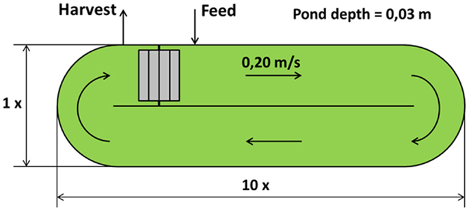
Figure 1. Raceway open pond.

Closed photobioreactors are designed to overcome the limitations of open systems. They have higher efficiency and biomass productivity, shorter harvesting times (2–3 days compared to 7–10 days for open pond), high surface-to-volume ratios, reduced contamination risks, and can be used to cultivate wider range of algal species than open systems (Bahadar and Bilal Khan, 2013). However, closed systems are more expensive to be constructed since they need high quality materials, and difficult to operate and scale up (Muñoz and Guieysse, 2006).

Flat panel photobioreactor is a flat, transparent vessel, made of glass, Plexiglas or plastic or other transparent material. The mixing of the water is carried out directly with air bubbling, which is introduced via a perforated tube at the bottom of the reactor. Flat panel PBRs are never thicker than 5–6 cm as the light entering the panel would not penetrate deeper in the culture. Only panels with both a height and width of <1 m have been studied (Janssen et al., 2003). The flat panel reactors are positioned vertically, closely spaced, to reach a higher photosynthetic efficiency through self-shading of the panels (Rawat et al., 2013). As for the open raceway pond, the main geometric characteristics have been taken from the literature (Janssen et al., 2003; Sierra et al., 2008; Pruvost et al., 2011; Ruiz et al., 2013; Kochem et al., 2014; Sugai-Guérios et al., 2014) and presented in Table 2 and Figure 2.

TABLE 2

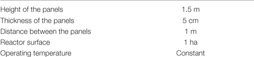
Table 2. Flat panel photobioreactor characteristics.

FIGURE 2

Figure 2. Flat panel photobioreactor.

Operating Strategy

The reactors can be operated either in continuous or in batch mode. The continuous operation requires a continuous extraction of the microalgae, while the batch operation extracts the produced microalgae after a certain time of production. An inoculum is, therefore, maintained in the reactor to serve as a basis for the new batch. The nutrient feeding strategy changes depending on the operating strategy: in continuous operation, two different reactors in series would be needed for lipid production, while in batch operation, a recipe for the batch feeding with nutrients has to be applied. As explained by Radmann et al. (2007), in the repeated batch cultivation after a certain period in the reactor, a specific culture volume is removed and replaced with an equal amount of fresh medium. Consequently, a part of cultivation medium is kept in the reactor as a starting inoculum. Repeated batch cultivation presents several operational advantages, the most important of which are the maintenance of a constant inoculum and high growth rates.

The operating strategy is also influenced by two considerations regarding the upstream and downstream processes. The downstream processing includes a settler tank where the extracted microalgae undergo a first concentration by sedimentation. The separated water is recycled while the products enter the downstream processing step. In this situation, the time required by the microalgae to grow can be decoupled from the time of the downstream technology. Second, in case of shortage of nutrients, the microalgae growth rate decreases as well as the production of new biomass, while the quantity of lipids in the biomass increases: this growth condition is particularly interesting if the downstream process aims at producing biodiesel. The models presented in this work do not consider the input condition of scarcity of nutrients, which instead are always supplied in excess.

Model

Cultivation Model Structure

The mass and energy produced by the cultivation systems in the form of biomass are calculated by the mathematical model through time-dependent mass and energy balances (Figure 3).

FIGURE 3

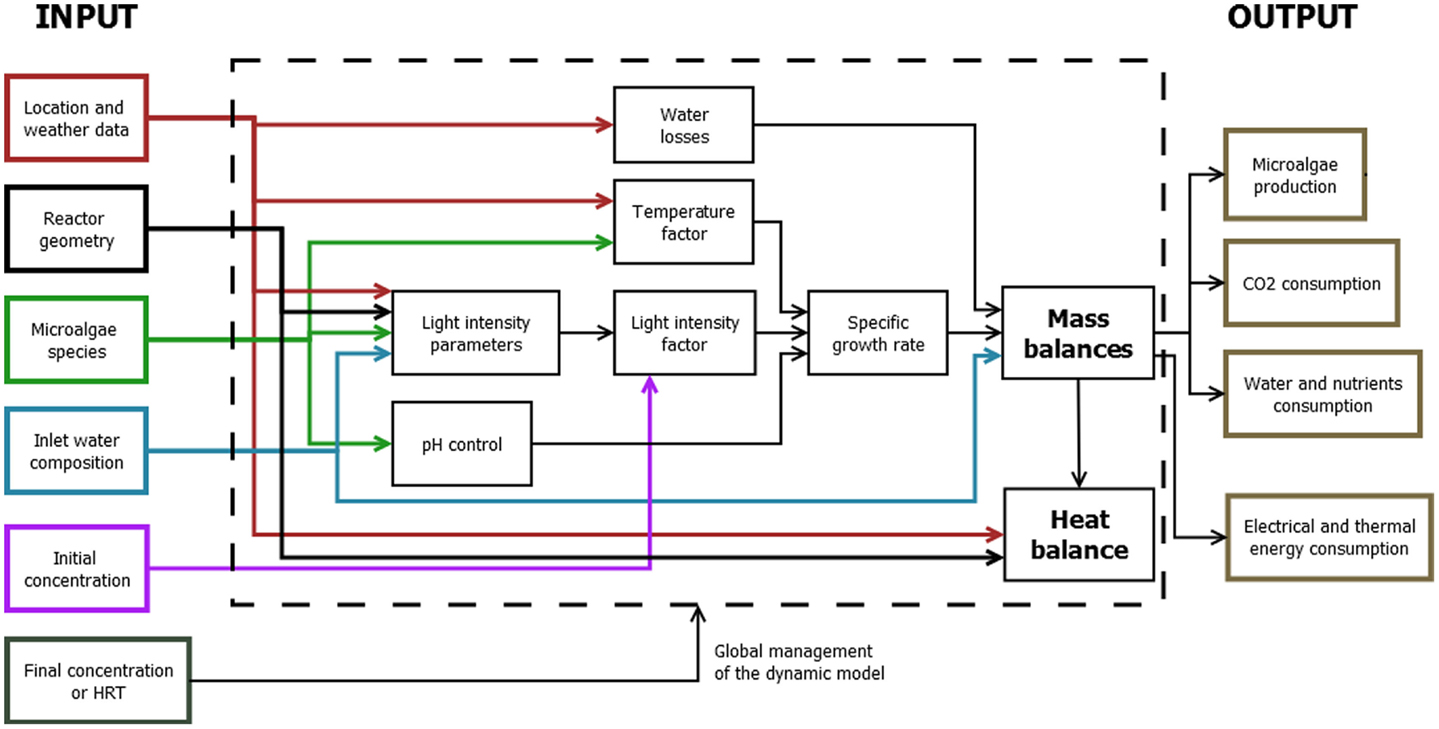
Figure 3. Model structure.

Before calculating the results of these balances, it is necessary to introduce some auxiliary equations. The auxiliary equations include the microalgae growth model, the pH control through CO₂ injection, and the equations to evaluate the radiation affecting the microalgae cells.

A set of differential equations is developed: it is solved by an explicit integration scheme with fixed time decomposition. To simplify the resolution of this system, the finite differences approximation was adopted. All the differential equations were treated as finite differences, and the backward difference formula was implemented

$\frac{\text{dx}}{\text{dt}}=f\left(t\right)\to \frac{x\left(t\right)-x\left(t-1\right)}{\Delta t}=f(t)$ (1)

This expression was preferred to the forward difference formula, being less vulnerable to instability.

If the backward difference formula is applied to matrices and vectors, the following expression is obtained:

$\overline{x}\left(t\right)=F\left(t\right)*\Delta t+\overline{x}\left(t-1\right)$ (2)

The model is a differential algebraic equations system that is converted into a set of algebraic equations by defining the proper solving sequence: some of the differential equations depend on one another, making impossible to solve them in a sequential logic: it is, therefore, necessary to solve them altogether as a system. Therefore, all the equations were manipulated to separate the known terms from the unknown variables and to obtain an easily solvable system of algebraic equations.

A dynamic approach to the resolution of energy and mass balances has been preferred to a steady state analysis because the laws describing the microalgae growth are time dependant; moreover, a dynamic model gives the opportunity of a deeper and more accurate evaluation of microalgae production and energy consumption over the time period.

Inputs to the Model

The following inputs are required by the model.

• Location data: latitude and longitude of the reactor are needed together with the hour difference between the location of the bioreactor and Greenwich.

• Weather data are also required by the model both to calculate the irradiation factor, which influences the microalgae growth and to evaluate the thermal balance. The open raceway pond model requires the global irradiation over a horizontal surface, whereas the flat panel model requires the direct and the diffuse radiation over a horizontal surface as two distinct data. Moreover, both the two models require other weather data, such as the atmospheric temperature, wind speed, and relative humidity. Hourly data are used in all models.

• Microalgae species characterization: many parameters of the model depend on this input, such as the maximum growth rate, the optimal growth temperature, and the saturation light irradiation. All the characteristics assume different values depending on the microalgae species. Table 3 presents the model parameters considered for two different microalgae strains. The model assumes a constant pH that is kept at the optimal value for microalgae species using CO₂ injection: to evaluate the correct quantities of CO₂ to be injected, the pH optimal value is represented as an optimal value of alkalinity of the reactor. LHV is the lower heating value for wet microalgae biomass. I_S is the saturation light intensity, μ_max is the maximum microalgae growth rate, T_let is the lethal temperature, T_opt is the optimal temperature for microalgae growth (maximum growth rate), and β is a curve modulating constant for the temperature factor. The decay rate is a coefficient that is used to evaluate the microalgae mass losses. K_C and K_NA are the half-saturation constants, i.e., the compound concentration when the specific growth rate [day⁻¹] is ${\mu }_{\text{A}}={\widehat{\mu }}_{\text{A}}/2$. From Yang (2011), K_C is set to $0.001{\text{mol}}_{{\text{CO}}_2}/{\text{m}}^3$ while K_NA = 0.001 mol_NA/m³. When nitrogen and carbon dioxide concentrations are next to the saturation values, these terms assume a value close to 1 and they do not affect the microalgae growth.

• The composition of the inlet water, which is used to fill the reactor at the beginning of each cultivation: since each cultivation cycle works as a batch reaction, nutrients must be supplied in sufficient quantities to feed the microalgae for the entire duration of the batch process. The model gives as input a surplus of nutrients in the water to guarantee they are not the limiting factor to microalgae growth. Then, as output, the model gives the exact quantity of nutrients consumed by the microalgae.

• The operating strategy, which is used to predict microalgae production. Two different strategies can be adopted: if the objective consists in searching the hydraulic retention time (HRT) required to reach a certain microalgae concentration in the reactor, the initial and the final microalgae concentrations are to be supplied as input information to the model. If the HRT is fixed along the whole time period, then the input data will be the initial concentration and the HRT, leaving the final concentration in the reactor free to change.

TABLE 3

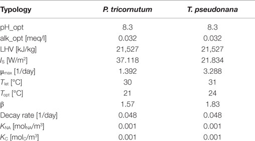
Table 3. Microalgae species characteristics.

Outputs of the Model

The mass production of microalgae is the most significant output of the cultivation model. In addition to this parameter, it is possible to define two other global performance parameters: the volumetric productivity {expressed in [g/(l × day)] or in [kg/(m³ × day)]} and the areal productivity {expressed in [t/(ha × y)] or in [kg/m² × day)]}. These parameters refer to the volume of the reactor and to the area of the soil covered by the reactor. Moreover, the model is able to give as output the exact quantities of all the compounds consumed or produced in the time period considered by the simulation (usually 1 year). For example, the model gives the CO₂ that is needed to be bubbled in the reactor to maintain a constant pH level and to feed the microalgae. In this way, the model gives the possibility to analyze the carbon footprint of the technology or at least to understand the quantity of CO₂, which can be fixed by the biomass produced, being a part of the injected CO₂ lost to the atmosphere: this quantity can be relevant in the case of open raceway pond.

Fundamental outputs of the model are the total electrical and thermal energies required by the reactor: to evaluate these quantities, the energy balance is not sufficient, as it is necessary to include the electrical energy spent at the boundary of the system, to refill the reactor and to harvest the biomass from the reactor itself; the electrical energy also includes the quantities which are needed for mixing and for the air bubbling in the bioreactor. Finally, another output of the model is the quantity of water required by the reactor, without considering the possible water recirculation coming from the downstream process.

Model Equations

Growth model. Following Yang (2011), the growth rate is calculated by Eq. (3):

$r_{\text{gA}}={\mu }_{\text{A}}{X}_{\text{A}}$ (3)

where X_A is the mass concentration of microalgae [g/m³] and μ_A is the specific growth rate [day⁻¹] that is calculated as:

${\mu }_{\text{A}}={\widehat{\mu }}_{\text{A}}\left(\frac{{\text{CO}}_{2\text{D}}}{K_{\text{C}}+{\text{CO}}_{2\text{D}}}\right)\left(\frac{N_{\text{T}}}{K_{\text{NA}}+N_{\text{T}}}\right)f_{\text{I}}{f}_{\text{T}}$ (4)

where the specific growth rate ${\widehat{\mu }}_{\text{A}}$ depends on the microalgae species; CO_2D, N_T are the quantities of dissolved nutrients and CO₂ [mol/m³] at time t. Nitrogen is the only nutrient that has been taken into account in the specific growth rate expression; other nutrients, such as phosphorus, are not explicitly considered, as suggested by Yang (2011), under the reasonable assumption that the metabolism of the microalgae is not limited or inhibited by these compounds. Although the growth rate may be affected by the presence of micro nutrients, they have not been introduced in the model to avoid the definition of a more complex reaction scheme with the corresponding experimental data to represent those influences. The specific growth rate can reach higher values thanks to the use of some micronutrients, such as iron and silicon (Chisti, 2007; Çelekli and Yavuzatmaca, 2009; Le et al., 2010; Ak, 2012; Bahadar and Bilal Khan, 2013). Nitrogen and CO₂ are considered limiting nutrients for microalgae growth and so microalgae growth rate dependence is expressed as saturation functions. K_C and K_NA are the half-saturation constants, as explained in the previous paragraphs. f_I is the light intensity factor representing the influence of the light on the microalgae production. Following Yang (Yang, 2011; Fernández et al., 2013), it is calculated by the following equation:

$f_{\text{I}}=\frac{I_{\text{a}}}{I_{\text{s}}}\text{exp}\left(1-\frac{I_{\text{a}}}{I_{\text{s}}}\right)$ (5)

where I_a is the average light intensity in the volume of the bioreactor at a given time t, while I_s is the saturation light intensity, which depends on the microalgae species being considered; saturation light intensity is usually in the range between 30 and 100 W/m² (Kumar et al., 2011). The average light intensity I_a depends on the weather, the turbidity caused by the microalgae and other substances in the water and on the reactor geometry. The model includes the hypothesis of perfect mixing: the whole quantity of microalgae in the water is affected by the same quantity of light radiation. f_T is the temperature factor. This term is equal to one and does not influence microalgae growth when the reactor temperature corresponds to the optimal growth temperature for the given microalgae species: this is what happens in the closed reactor, where a heat exchanger is used to keep a constant optimal temperature. Below and above the optimal growth temperature, the growth is negatively influenced by the water temperature. Above the optimal temperature, the value of f_T decreases fast and reaches 0 for a certain temperature that again depends on the algae species: this value is called lethal temperature (T_let). The expression of the temperature factor is shown in the following equation, taken from Slegers et al. (2013):

$f_{\text{T}}={\left(\frac{T_{\text{let}}-T_{\text{w}}}{T_{\text{let}}-T_{\text{opt}}}\right)}^{{\beta }_{\text{algae}}}\text{exp}\left(-{\beta }_{\text{algae}}\left(\frac{T_{\text{let}}-T_{\text{w}}}{T_{\text{let}}-T_{\text{opt}}}-1\right)\right)$ (6)

β_algae depends on the algae species and it is a curve modulating constant.

Figure 4 shows the shape of the temperature factor f_T: it is possible to note that the equation used for the temperature factor suggested by Slegers et al. (2013) overestimates the growth for low temperature values, since the growth is not possible for low temperatures.

FIGURE 4

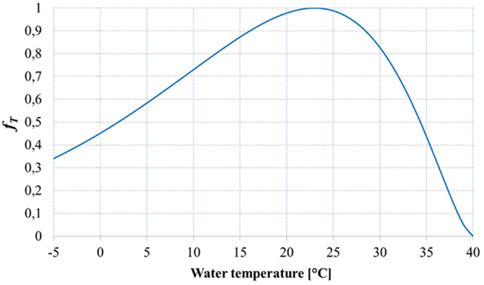
Figure 4. Temperature factor (Slegers et al., 2013).

pH control strategy. Each microalgae species has an optimal pH value: the model includes a control system to keep the optimal value of pH in the reactor through CO₂ injection. As shown in the following equations from Sills (2013), the pH can be controlled by keeping constant two parameters: dissolved CO₂ concentration and alkalinity. Since alkalinity does not change with time in the model, to keep pH constant, it is necessary to calculate the quantity of dissolved CO₂ which has to be maintained constant during time.

The total concentration (C_T) of carbonate species in solution is defined as

$C_{\text{T}}=\left[{\text{H}}_2{\text{CO}}_3^{*}\right]+\left[{\text{HCO}}_3^{-}\right]+\left[{\text{CO}}_3^{2-}\right]$ (7)

Dissolved CO₂ concentration is $\left[{\text{CO}}_{2(\text{ag})}\right]\cong \left[{\text{H}}_2{\text{CO}}_3^{\text{*}}\right].$ The molar concentration of each carbonate species (as a fraction of C_T) depends on pH, according to the following equations:

$\left[{\text{H}}_2{\text{CO}}_3^{*}\right]=\frac{C_{\text{T}}}{1+\frac{k_1}{\left[{\text{H}}^{+}\right]}+\frac{k_1{k}_2}{{\left[{\text{H}}^{+}\right]}^2}}={\alpha }_0{C}_{\text{T}}$ (8)

$\left[{\text{HCO}}_3^{-}\right]=\frac{C_T}{1+\frac{\left[{\text{H}}^{+}\right]}{k_1}+\frac{k_2}{\left[{\text{H}}^{+}\right]}}={\alpha }_1{C}_T$ (9)

From Eqs (8) and (9), α₀ and α₁ are calculated.

$\left[{\text{CO}}_3^{2-}\right]=\frac{C_T}{1+\frac{\left[{\text{H}}^{+}\right]}{k_2}+\frac{{\left[{\text{H}}^{+}\right]}^2}{k_1{k}_2}}={\alpha }_2{C}_T$ (10)

Finally:

$C_{\text{T}}=\frac{\text{alk}-{\text{OH}}^{-}+{\text{H}}^{+}}{{\alpha }_1+2{\alpha }_2}$ (11)

Since pH is the concentration of dissolved [H⁺] in the water and pH = 14 − pOH, all terms are known and the total concentration of carbonate species can be obtained by

$C_{\text{T}}=\frac{\text{alk}-{\text{OH}}^{-}+{\text{H}}^{+}}{{\alpha }_1+2{\alpha }_2}$ (12)

This term will be a part of the time-dependent CO₂ mass balance, which is used to calculate the CO₂ injection at each time t.

Mean light intensity for open pond. The light intensity factor in the specific growth rate expression contains I_a, that is the average light intensity in the bioreactor at a given time. Starting from global horizontal radiation, the model evaluates I_a using the Beer–Lambert’s law, which assumes an exponential decay of the light intensity from the external surface of the cultivation system:

$I_{\text{a}}\left(s\right)=I_0\text{exp}\left(-\sigma X_{\text{A}}s\right)$ (13)

As it is explained by Béchet et al. (2013), I_a(s) is the local light intensity, s is the distance from the external surface of the system to the position under consideration, I₀ is the incident light intensity, σ is the extinction coefficient, and X_A the cell concentration. The Beer–Lambert’s law can be applied only if two conditions are verified by the culture medium: first, it must be isotropic (i.e., the optical properties of the broth are independent from light direction); this condition is often verified in well-mixed systems. Second, algae cells should not scatter light: this second condition is not always met, but the model considers both the two requirements always verified. The equations to calculate I_a strictly depend on the geometry of the bioreactor: for the open pond, as suggested by Yang (2011), an integration through the pond depth of the Beer–Lambert’s law has been used:

$I_{\text{a}}=\frac{1}{Z}\underset{0}{\overset{\text{Z}}{{\displaystyle \int }}}{I}_0\text{exp}\left(-K_{\text{e}}z\right)\text{dz\hspace{0.17em}}$ (14)

where I₀ is obtained directly from the global horizontal radiation I_GHR: I₀ = PAR × I_GHR. PAR is the photosynthetic active radiation (PAR), i.e., the amount of solar radiation which is used by the microalgae for the photosynthesis and which corresponds to 45% of the total incoming light. K_e is related to algal concentration in the pond, and it is called extinction coefficient:

$K_{\text{e}}=K_{\text{e}1}+K_{\text{e}2}{X}_{\text{A}}$ (15)

Light intensity for flat panel. In case of flat panel, the complexity of the geometry requires the use of different equations from those applied for the open pond. The equations used to calculate the light intensity for flat panels are taken from Slegers et al. (2011). For this typology of reactors, the input data are the direct and diffuse radiation on the horizontal surface; moreover, the equations must take into account also the reflection of the radiation on the surface of the panel. As explained by Slegers et al. (2011), to evaluate the effect of direct light irradiation over a tilted surface (panels positioned vertically), it is necessary to introduce a geometrical parameter for direct radiation:

$G_{\text{direct}}\left(t\right)=\frac{\cos \theta }{\cos {\theta }_{\text{z}}}$ (16)

in which θ is the solar incidence angle, and θ_z is the solar zenith angle. The values assumed by these angles during each day of the year depend on the location, and have been calculated using the equations taken from Duffie and Beckman (2013).

For large scale cultivations, parallel positioned flat panels are used. Parallel placement causes shading, and consequently part of the panels no longer receive direct sky light. The shadow height on vertical reactor panels is given by

$h_{\text{shadow}}=h-\frac{d\tan \left(90-{\theta }_{\text{z}}\right)}{\cos \left(\text{γ}\right)}$ (17)

which is a function of the reactor height h [m], distance between the reactor panels d [m], solar elevation, which is equal to 90 − θ_z and angle between solar rays and the azimuth of the surface. If h_shadow > 0, the flat panel is divided into two parts. The upper part receives direct and diffuse radiation, the lower part only diffuse light. The separation between the upper and the lower part varies with the solar position. Parallel placement of the reactors also influences the penetration of diffuse sky light into the space between panels; the light intensity decreases from the top to the bottom. A similar situation can be seen with the penetration of light in urban street canyons (Robinson and Stone, 2004). For these reasons, the geometrical factor for diffuse light depends on the position over the surface of the panel.

At height y < h_shadow:

$G_{\text{diffuse}}=\frac{1+\cos \left(\beta +u\right)}{2}$ (18)

where u = atan(y/d), β [deg] is the slope of the reactor, i.e., the angle that the surface makes with the surface of the earth.

At height y > h_shadow:

$G_{\text{diffuse}}=\frac{1+\cos (\beta )}{2}$ (19)

All panels are treated similarly in the calculations. Moreover, ground reflection is low for parallel placed panels, and is therefore not taken into account.

The total amount of light falling on each reactor surface at a given height y, of a given time t is:

$I_0\left(y,t\right)=G_{\text{direct}}\left(t\right)I_{\text{direct}}\left(t\right)+G_{\text{diffuse}}\left(y\right)I_{\text{diffuse}}\left(t\right)$ (20)

At this point, it is fundamental to consider the reflected fraction of the irradiation, which does not enter into the reactor and so does not contributes to the microalgae growth. The amount of reflected light on each interface is related to the differences in refractive indices and the incidence angle (Sukhatme and Sukhatme, 1996).

The incidence angle for diffuse radiation which is considered to evaluate the light reflection is assumed to be 60°, as it is suggested by Duffie and Beckman (2013).

Light reflection by the flat panel walls follows Fresnel equations:

$R_{\text{s}}={\left[\frac{{\eta }_{\text{i}}\cos \left({\theta }_{\text{i}}\right)-{\eta }_{\text{t}}\sqrt{1-{\left(\frac{{\eta }_{\text{i}}}{{\eta }_{\text{t}}}\sin \left({\theta }_{\text{i}}\right)\right)}^2}}{{\eta }_{\text{i}}\cos \left({\theta }_{\text{i}}\right)+{\eta }_{\text{t}}\sqrt{1-{\left(\frac{{\eta }_{\text{i}}}{{\eta }_{\text{t}}}\sin \left({\theta }_{\text{i}}\right)\right)}^2}}\right]}^2$ (21)

$R_{\text{p}}={\left[\frac{{\eta }_{\text{i}}\sqrt{1-{\left(\frac{{\eta }_{\text{i}}}{{\eta }_{\text{i}}}\sin \left({\theta }_{\text{i}}\right)\right)}^2}-{\eta }_{\text{t}}\cos \left({\theta }_{\text{i}}\right)}{{\eta }_{\text{i}}\sqrt{1-{\left(\frac{{\eta }_{\text{i}}}{{\eta }_{\text{i}}}\sin \left({\theta }_{\text{i}}\right)\right)}^2}+{\eta }_{\text{t}}\cos \left({\theta }_{\text{i}}\right)}\right]}^2$ (22)

where θ_i [°] is the incidence angle, η_i [−] is the refractive index of the material before the interface, and η_t [−] is the refractive index for the material after the interface. Normal sunlight is non-polarized, therefore the overall reflection coefficient equals the average of the reflection coefficients for s-polarized and p-polarized light:

$R^{\prime }=\frac{R_s+R_p}{2}$ (23)

The light reflected within the reactor wall is completely transmitted to the air, introducing the hypothesis of a non-absorbing material for the walls of the reactor. The light transmitted to the culture, which has to be calculated separately for direct and diffuse radiation, is

$I_{\text{i}}(t)=I_0(t)(1-{R^{\prime }}_1{R^{\prime }}_2)T_{\text{m}}$ (24)

T_m [−] is a factor which takes into account a possible low transparency of the material.

The calculation is performed for both the two sides of the reactor and, for parallel positioned panels, for each height. R₁′ and R₂′ are the reflection coefficients for the air–reactor wall interface and the reactor wall–culture volume interface, respectively. Two light intensity gradients exist in the culture volume. First, as a function of height due to shading and the penetration of diffuse light between parallel positioned panels. Second, in the liquid between the two reactor walls. The second gradient runs from the reactor wall to the center of the reactor and is caused by the absorption of light by the medium and the algae (Slegers et al., 2011). Only the PAR of the spectrum is absorbed by the algae. This accounts for about 45% of the total light. The Lambert–Beer’s law is used for the overall light gradient in the culture volume, as it was done for the open pond:

$I\left(y,z,t\right)=I_{\text{front}}{e}^{-\left(K_{\text{e}1}+K_{\text{e}2}{X}_{\text{A}}\right)z}+I_{\text{back}}{e}^{-\left(K_{\text{e}1}+K_{\text{e}2}{X}_{\text{A}}\right)\left(s-z\right)}$ (25)

This equation gives the light intensity at location z [m] inside the reactor thickness [m], at a given height y [m] in the reactor at time t.

At this point, to simplify the model, the values of light intensity I(y,z,t) are integrated to find a mean value of irradiation for the whole culture inside the whole reactor at a given time t: with these integrations, a single value of radiation is obtained and used in the growth model, for the whole panel, at a given time t. The hypothesis of a perfect mixing inside the culture at each time t is necessary to integrate the equation in both height and depth.

Mass balances. Mass balances of nitrogen and oxygen inside the pond can be modeled in the same way, suggested by Yang (2011):

$\frac{\text{dM}}{\text{dt}}={\mu }_{\text{A}}{X}_{\text{A}}{Y}_{\text{AM}}-k_{\text{Lg}}\alpha \left(M-M^{*}\right)$ (26)

where M is the concentration of the respective component in the water in the bioreactor, Y_AM is the mass of the respective component consumed or generated by the microalgae per unit mass of microalgae produced. The last term of the right-end side of Eq. (26) represents the mass transfer between the atmosphere and the pond, where k_Lgα is the mass transfer coefficient for a given element, M* is the saturation concentration of the associated dissolved element.

For total inorganic carbon, the mass balance assumes a different formulation since the CO₂ is injected continuously in the pond during the growth phase to keep a constant concentration of dissolved CO₂ in the reactor, balancing the losses of CO₂ to the atmosphere and the consumption of CO₂ by the microalgae.

$\frac{{\text{dCO}}_2}{\text{dt}}={\mu }_{\text{A}}{X}_{\text{A}}{Y}_{{\text{ACO}}_2}+f_{{\text{CO}}_2}-k_{\text{Lg}}\alpha \left({\text{CO}}_2-{\text{CO}}_2{}^{*}\right)$ (27)

where $f_{{\text{CO}}_{\text{2}}}$ represents the flux of CO₂ introduced by the supply of gas flow into the system. Since the quantity of dissolved CO₂ is kept constant (dCO₂/dt = 0), the mass balance can be written again as

$f_{{\text{CO}}_2}=-{\mu }_{\text{A}}{X}_{\text{A}}{Y}_{{\text{ACO}}_2}+k_{\text{Lg}}\alpha \left({\text{CO}}_2-{\text{CO}}_2{}^{*}\right)$ (28)

Finally, the mass balance for microalgae species can be written as

$\frac{{\text{dX}}_{\text{A}}}{\text{dt}}={\mu }_{\text{A}}{X}_{\text{A}}-k_{\text{dA}}{X}_{\text{A}}$ (29)

As it can be seen, all these equations are time dependent, and all strictly depend on one another: this means that they form altogether a system of differential equations. The strategy to solve the equations with the finite difference methodology is used to solve this system in Matlab, and therefore to solve the system of differential equations as a system of algebraic equations.

Thermal balance for open pond. The model includes the thermal balance as it is suggested by Slegers et al. (2013):

$V_{\text{R}}{\text{cp}}_{\text{w}}{\rho }_{\text{w}}\frac{{\text{dT}}_{\text{w}}}{\text{dt}}=Q_{\text{irr}}-Q_{\text{algae}}-Q_{\text{rad}}-Q_{\text{evap}}-Q_{\text{conv}}-Q_{\text{cond}}$ (30)

where V_R is the volume of the pond, cp_w the heat capacity of the growth medium, ρ_w the density of the growth medium, T_w the temperature in the pond, Q_irr the heat flow rate to the pond by the sunlight, Q_algae the light energy flow rate to algae during growth, Q_rad the heat flow rate by emission of long-wave radiation in the infrared region, Q_evap [W] the heat flow rate caused either by evaporation or condensation, Q_conv the heat flow rate by convection, and Q_cond the heat flow rate between pond and ground via conduction. The water in the pond is heated by sunlight that enters the culture volume. Solar energy that is not used by algae for growth is considered as thermal energy that is dissipated through the different thermal exchange mechanisms (Q_rad, Q_evap, Q_conv, and Q_cond) or as a contribution to temperature growth in the pond. The total heat flow rate by the sunlight is given by

$Q_{\text{irr}}=A_{\text{w}}{I}_{\text{surface}}\left(t\right)$ (31)

where A_w [m²] is the water surface area of the pond and I_surface [W/m²] is the total light arriving on the pond. Part of this light is absorbed by microalgae for growth:

$Q_{\text{algae}}=h_{\text{comb}}{\mu }_{\text{A}}{X}_{\text{A}}{V}_{\text{R}}$ (32)

which is a function of the lower heating value on a dry basis of algae biomass h_comb [J/kg], specific growth rate μ_A [s⁻¹] and the biomass concentration X_A [kg/m³].

The water in the pond emits thermal energy by long-wave radiation. The overall long-wave radiation flow between water in the pond and sky is calculated using Duffie and Beckman (2013):

$Q_{\text{rad}}={\text{A}}_{\text{w}}{\epsilon }_{\text{w}}{\sigma }_{\text{SB}}\left({\left(T_{\text{w}}+273.15\right)}^4-T_{\text{sky}}^{\text{4}}\right)$ (33)

where ϵ_w [−] is the emissivity of the water in the infrared region, σ_SB [W/(m²K⁴)] the Stefan–Boltzmann constant, and T_sky [K] the equivalent sky temperature for clear sky days, which is expressed by Duffie and Beckman (2013) as

$T_{\text{sky}}=(T_{\text{a}}+273.15){(0.711+0.0056T_{\text{dew}}+0.000073T_{\text{dew}}^2+0.013\text{cos}(15t_{\text{solar}}\text{))}}^{\text{0.25}}$ (34)

where T_a [°C] is the air temperature, T_dew [°C] the dew point temperature, and t_solar [−] the number of hours after solar midnight.

Evaporation has a large effect on the water temperature, especially in locations with low humidity and high wind velocities. The evaporation rate depends on the shape of the water area, wind velocity, and consequently also movement of the water. The evaporation flow is driven by the difference of water vapor pressures between ambient air the saturated water body. The evaporation energy flow is given by

$Q_{\text{evap}}=A_{\text{w}}{h}_{\text{evap}}(p_{\text{s}}^{\text{'}}-p_{\text{a}}^{\text{'}})$ (35)

The evaporation flow depends on the heat transfer coefficient for evaporation h_evap [W/(m² Pa)], the saturated water pressure p′_s [Pa] at water temperature T_w, and the water pressure of air p′_a [Pa] at air temperature T_a. The evaporation rates have been calculated using the heat transfer coefficient h_evap found in Duffie and Beckman (2013):

$h_{\text{evap}}=0.036+0.025v$ (36)

where v [m/s] is the wind speed. The Antoine equation is applied to calculate the saturated water pressure p′_s [Pa] at water temperature T_w and the water pressure of the air p′_a [Pa] at air temperature T_a:

$p^{\prime }=\text{RH\hspace{0.17em}}{10}^{\left(8.07131+{\text{log}}_{10}\left(\frac{101325}{760}\right)\right)-\frac{1730.63}{233.46+T_{\text{a}}}}$ (37)

where RH [−] is the relative humidity and T_a [°C] the temperature.

Convection and evaporation are related processes, as it is shown in Eq. (37). The flow for passive and forced convection at the water surface mainly depends on the difference between water and air temperature. The convection flow is given by

$Q_{\text{conv}}=C_{\text{Bowen}}\frac{p_{\text{a}}\left(T_{\text{w}}-T_{\text{a}}\right)}{p_{\text{ref}}\left({p^{\prime }}_{\text{s}}-{p^{\prime }}_{\text{a}}\right)}{Q}_{\text{evap}}$ (38)

where C_Bowen is the Bowen constant [Pa/°C], p_a is the ambient pressure [Pa] and p_ref the reference pressure [Pa], and p′_s and p′_a are derived using equation

$p^{\prime }=\text{RH\hspace{0.17em}}{10}^{\left(8.07131+{\text{log}}_{10}\left(\frac{101325}{760}\right)\right)-\frac{1730.63}{233.46+{\text{T}}_{\text{a}}}}$ (39)

Conductive heat transfer takes place between the open pond and the soil. The soil is assumed to be an infinite source for heat transfer. This heat transfer calculation is derived from Fourier’s law:

$Q_{\text{cond}}=h_{\text{soil}}{A}_{\text{soil}}\left(T_{\text{w}}-T_{\text{soil}}\right)$ (40)

where h_soil [W/(m²°C)] is the heat transfer coefficient of the surrounding soil layer, A_soil [m²] is the area of the pond that is embedded in the soil, and T_soil [°C] is the temperature of the soil surrounding the pond.

Thermal balance for flat panel. Due to the significant difference in the geometry of the reactor and the temperature strategy being considered, the thermal balance for the flat panel assumes a different form from that implemented for the open raceway pond:

$V_{\text{R}}{\text{cp}}_{\text{w}}{\rho }_{\text{w}}\frac{{\text{dT}}_{\text{w}}}{\text{dt}}=Q_{\text{irr}}-Q_{\text{algae}}-Q_{\text{exch}}-Q_{\text{conv}+\text{cond}}$ (41)

In a flat panel, a constant value of the water temperature T_w [°C] is desired, and obtained using a heat exchanger placed at the bottom of the reactor to remove or supply heat.

Thus, the thermal balance can be written as follows:

$\frac{{\text{dT}}_{\text{w}}}{\text{dt}}=0\to Q_{\text{irr}}-Q_{\text{algae}}-Q_{\text{exch}}-Q_{\text{conv+cond}}=0$ (42)

Q_irr [W] is given by the following expression:

$Q_{\text{irr}}=2A_{\text{panel}}{I}_{\text{mean}}$ (43)

where A_panel is the surface of the reactor, which is multiplied by two, as it is necessary to consider both the front and the back surfaces; I_mean [W/m²] is the radiation previously calculated taking into account both the direct and diffuse radiation and the reactor geometry that is the radiation which interacts with the water in the reactor and with the microalgae. As calculated for the open pond, a part of the incoming heat is used by the microalgae for growing:

$Q_{\text{algae}}=h_{\text{comb}}{\mu }_{\text{A}}{X}_{\text{A}}{V}_{\text{R}}$ (44)

which is a function of the combustion energy of algae biomass h_comb [J/kg], specific growth rate μ_A [s⁻¹], biomass concentration X_a [kg/m³], and reactor volume V_R [m³].

The model takes into account the natural convection over the panel surface caused by the wind and the glass conductivity:

$Q_{\text{conv}+\text{cond}}=2A_{\text{panel}}{U}_{\text{tot}}\left(T_{\text{w}}-T_{\text{atm}}\right)$ (45)

where

$U_{\text{tot}}=U_{\text{cond}}+U_{\text{conv}}$ (46)

where U_cond is the glass conductivity [W/(m²K)] and U_conv is the conductivity of the natural convection that is obtained by Duffie and Beckman (2013). Using the equations above, the quantity of heat that has to be removed or supplied by the heat exchanger at each time t can be calculated. Heat exchange through radiation can be omitted from this balance, since the water temperature is always kept between 20 and 30°C, depending on microalgae growth optimal temperature.

Electrical energy consumption for harvesting, refilling, mixing and bubbling. For both the open pond and flat panel, the harvesting of the water from the reactor and its refilling are carried out in 8 h, during one night: 3.5 h are required for harvesting and 3.5 h for refilling. These operations are performed using a pump. The electrical consumption has been calculated as follows:

$E_{\text{harv/refil}}=P_{\text{pump}}{t}_{\text{harv/refil}}$ (47)

where the power of the pump is

$P_{\text{pump}}=\frac{\rho gQh}{{\eta }_{\text{pump}}}$ (48)

where ρ is the water density [kg/m³], g is the acceleration of gravity [m/s²], η_pump [−] is the efficiency of the pump, set at 0.85, Q [m³/s] is the volumetric flow rate which has to be pumped, and h [m] is the height difference between the two basins before and after the pump: thanks to the fact that the model includes also the design of a settler positioned after the bioreactor, it is possible to know the exact h for the harvesting, which has been increased to consider the losses in the pipes, whereas for the refilling data have been taken from the literature, considering h = 1 m for the open pond and 3 m for the flat panel: the difference between these two values is again associated with the energy losses in pipes.

The power required for mixing in the open pond is

$P_{\text{mix}}=\frac{\rho gQh}{{\eta }_{\text{paddlewheel}}}$ (49)

where Q [m³/s] is obtained from the water speed that is desired in the reactor (0.20 m/s) and from the cross-section of the open pond (which depends on the geometry), h is the given height difference before and after the paddle wheel, taken from literature (0.05 m). η_paddlewheel is lower than the efficiency of a normal pump and is assumed to be equal to 0.25.

Both for the open pond and flat panel, a bubbling system has to be taken into account: for the flat panel, this system should be able both to supply the CO₂ necessary for the photosynthesis of the microalgae and to guarantee an adequate mixing inside the reactor. For this reason, the amount of air bubbled in the flat panel is higher than the air supplied to the open pond. These quantities are controlled by the CO₂ molar fraction inside the injected air which is 0.04 in the case of open pond and 0.02 for the flat panel. The design and the energy consumption of the bubbling system have been calculated through Belsim Vali modeling software, using a compressor. The result is that it is necessary to supply 4 kJ for each kg of air injected in the reactor.

Results

Open Pond

Tables 4 and 5 show the input and output data in the open pond modeling:

TABLE 4

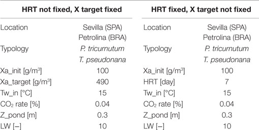
Table 4. Input data for open pond simulations.

TABLE 5

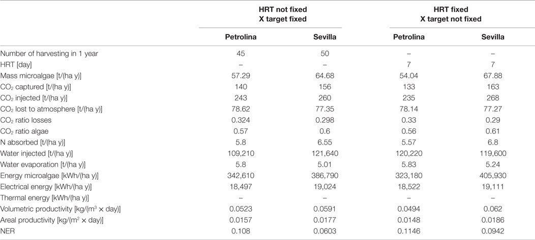
Table 5. Output from open pond simulations.

The open pond productivity that is obtained by the model is consistent with the literature: Slegers et al. (2013) estimated an annual biomass production for a 1 ha surface in the Netherlands and Algeria equal to 41.5 and 63.7 t, respectively. Fernández et al. (2013) report a maximum microalgae areal productivity equal to 30 g/(m² day), higher than those resulting from the model calculations, but still of the same order of magnitude. Jiménez et al. (2003) obtained a volumetric productivity equal to 0.05 kg/(m³ day) for a location in Southern Spain (Malaga), by cultivating the microalgae until a maximum concentration of 470 g/m³: the cultivation conditions and the results from the dynamic model are consistent with the results of this work.

In this work, the Net Energy Ratio (NER)

$\text{NER}=\text{Net\hspace{0.17em}Energy\hspace{0.17em}Ratio}=\frac{\text{total energy requirement for operation}}{\text{total\hspace{0.17em}energy\hspace{0.17em}production\hspace{0.17em}(biomass)}}$ (50)

expresses the fraction of the energy produced in the cultivation system that is used by the system itself to generate the biomass. If this value is close to 1, the cultivation technology of microalgae is too energy intensive, requiring a big share of the energy produced. From Table 5, it appears that for both the locations analyzed by the model the NER is quite far from 1, showing that the energy demand for the operation of the cultivation system in Petrolina is 10.8% of the energy contained in the biomass produced, while for Sevilla is 6%. These values are quite promising for a potential production of microalgae in these locations, since the NER is far enough from 1: even if the energy content of open pond construction and materials are added to the total energy requirement, it seems reasonable to state that the plant would still be convenient from an energetic point of view. Another important output of the model from an environmental point of view is the quantity of CO₂ fixed by the microalgae during the growth process: the downstream process that transforms microalgae biomass into biofuel releases CO₂ to the atmosphere, with a negative environmental impact. Since the cultivation phase captures more CO₂ than the quantity released, using the data of CO₂ fixed in the algae it is possible to calculate a global CO₂ balance, for the entire biofuel production chain: this environmental analysis may lead to a comparison with other biofuel chain production and with traditional fossil fuels, to evaluate which product has a positive or negative environmental impact.

With the first operating strategy (meaning that the inputs are the initial and final concentration), one of the output would be the number of days that are needed to reach the final target concentration. The number of days is not the same along the year, being variable with weather conditions. During wintertime, the harvesting period in Sevilla is extremely long due to low irradiation and low temperatures, which make the microalgae growth in the pond slow and difficult. A possible strategy to overcome this limitation might be to interrupt the production during wintertime: in this case, the productivity during the whole year would decrease, since a part of the biomass would not be produced, but the NER would positively decrease, because of the absence of energy consumption during winter: the production lost is less than the energy saving obtained, and so the overall effect would be positive. For Petrolina, the HRT is more homogeneous along the year, but longer: the reason might be that weather conditions in Petrolina cause a strong increase of pond temperature that may cause a consequent reduction in microalgae productivity when pond temperature is higher than the optimal temperature for microalgae growth.

Results of dynamic simulation runs are reported in Figures 5–9, showing the effect of PAR and pond temperature over the specific growth rate and microalgae growth rate. Input parameters for simulation runs are shown in Table 6.

FIGURE 5

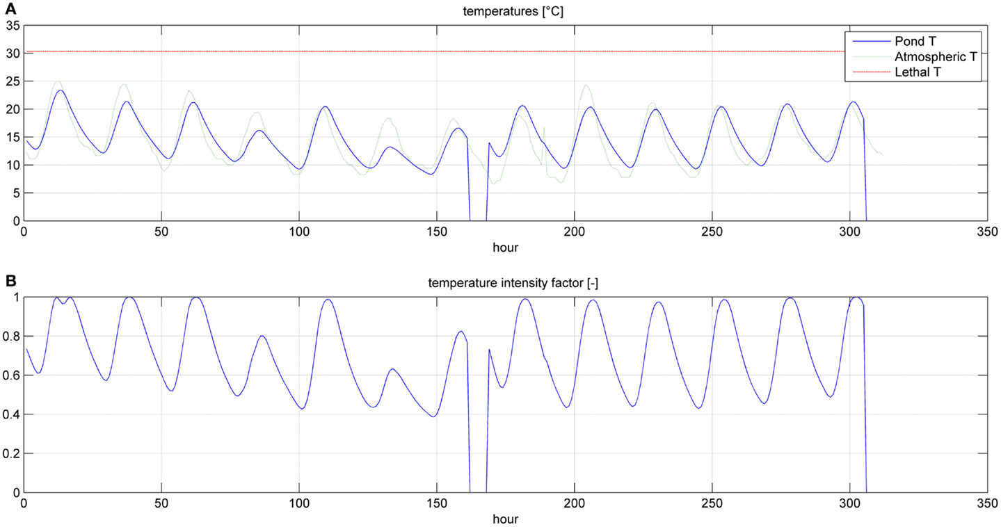
Figure 5. Temperatures (A) and temperature factor (B) for a simulation time equal to two HRTs.

FIGURE 6

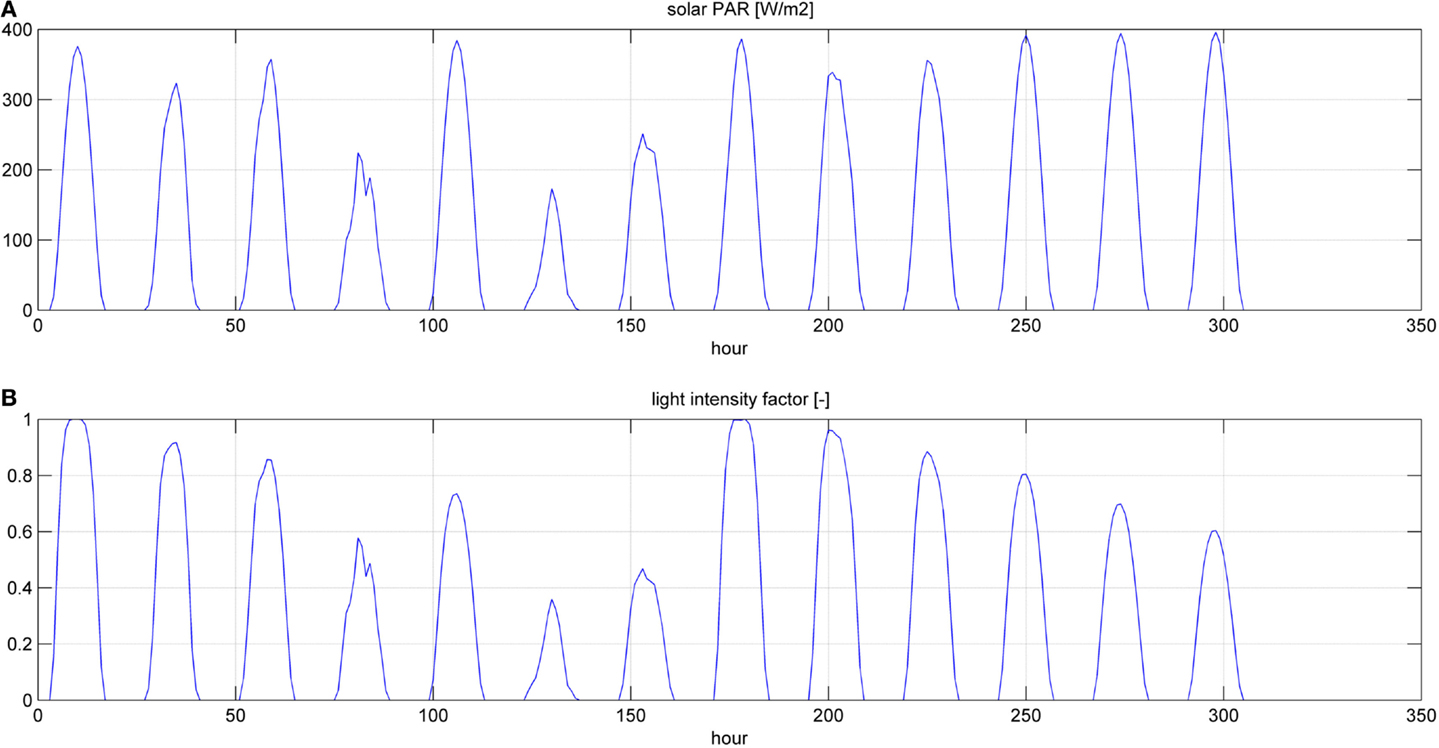
Figure 6. Photosynthetic active radiation (PAR) (A) and light intensity factor (B) for a simulation time equal to two HRTs.

FIGURE 7

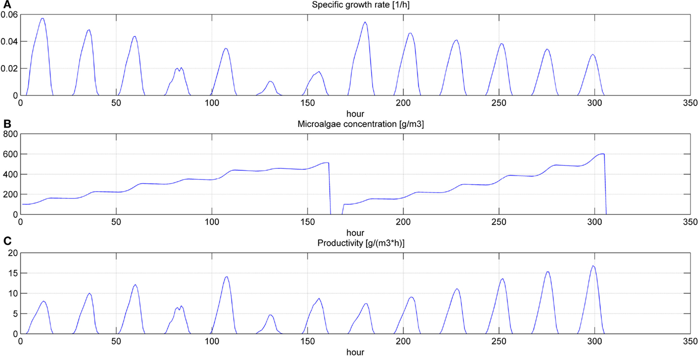
Figure 7. Specific growth rate (A), microalgae concentration (B) and microalgae volumetric productivity (C) in the open pond during two consequent batch cultivations (simulation time equal to two HRTs).

FIGURE 8

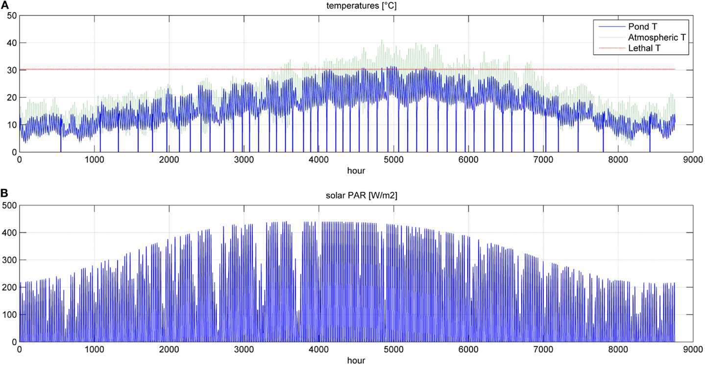
Figure 8. Temperatures (A) and photosynthetic active radiation (B) for a simulation time equal to 1 year.

FIGURE 9

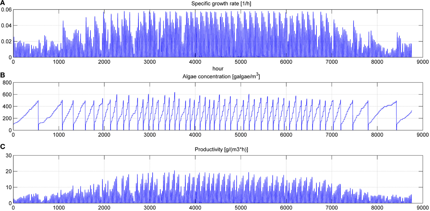
Figure 9. Specific growth rate (A), microalgae concentration in the pond (B) and microalgae growth rate (C) for a simulation time equal to 1 year.

TABLE 6

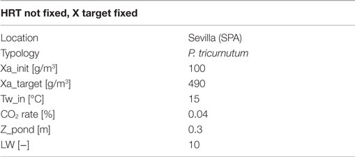
Table 6. Input data for open pond simulation runs.

Even if the simulation has been run for the entire year, as it is shown in Figures 8 and 9, Figures 5–7 report a small time range that includes two consequent batch cultivations, for an easier understanding of the light and temperature effect over the microalgae growth. Figure 5 includes the pond temperature values (A), calculated in each hour of the entire simulation period, and the consequent temperature factor (B). In Figure 5, the model does not evaluate the pond temperature during the hours when the pond is emptied. Figure 6 reports the PAR and the consequent light intensity factor (B). Figure 7 shows the specific growth rate (A) and the microalgae concentration (B) in the open pond during two consequent batch cultivations. Microalgae growth rate (C) is obtained, as explained in Eq. (3), by the product of the specific growth rate and the microalgae concentration. As shown in Figure 7B, each batch cultivation starts with the same initial concentration, while the final concentration depends on each batch: the model waits for the end of the solar radiation to start to empty the pond that takes almost the whole night.

In Figures 8 and 9, the time of the entire simulation run has been considered presenting input values (temperature in Figure 8A and PAR in Figure 8B) and output [specific growth rate in Figure 9A, microalgae concentration in the pond in Figure 9B and microalgae growth rate (productivity) in Figure 9C].

The time to reach the minimum microalgae target concentration to start the harvest in winter time in Sevilla is really long and it might be useful to interrupt the production for some months.

Flat Panel

Table 7 shows the input data for the flat panel model for both the two operating strategies.

TABLE 7

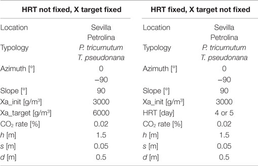
Table 7. Input data for flat panel simulations.

The azimuth of the panel is an input, which may vary from 0°, when the panel faces south, to −90°, when the panel faces east. The model is not able to consider different slopes of the reactor, which may only be positioned vertically: this position is the most favorable for light distribution and dilution, leading to the highest values of productivity (Sierra et al., 2008). CO₂ molar concentration in the injected gases is lower than that of the open raceway pond, since the injected gases in the flat panel photobioreactor do not only have to supply the CO₂ needed by microalgae for photosynthesis, but also to generate the necessary mixing in the reactor: adequate mixing is essential to obtain good levels of productivity in every microalgae cultivation system. Due to the complex geometry of the flat panel photobioreactor, more geometrical data are needed as input if compared to the open raceway pond system. As explained by Fernández et al. (2013), heights <1.5 m and widths <0.10 m are preferred; following this indication and data from Slegers et al. (2011), the distance between the vertical panels has been set equal to 0.5 m, the height of each panel to 1.5 m and the thickness to 5 cm. Both height and distance between panels have been varied within a range of possible values in a further parametrical analysis. The initial and final concentrations have been suggested by Münkel et al. (2013); the values are higher than in the case of open raceway pond: the more sophisticate closed photobioreactor allows higher concentrations to be reached without compromising the productivity of the cultivation system. This is possible thanks to an optimal light distribution over the whole reactor for the entire operation time that is guaranteed also by an adequate mixing of the medium. The flat panel model, as well as the open raceway pond model, is able to produce the dynamic trend of all the time dependent physical quantities, which are included in the analysis. The global results for the flat panel reactor are shown in Tables 8 and 9: Table 8 reports the results for the first operating strategy, i.e., the case in which both input and output microalgae concentrations are known, whereas Table 9 corresponds to the second operating strategy, in which the input parameters are the input concentration and the HRT.

TABLE 8

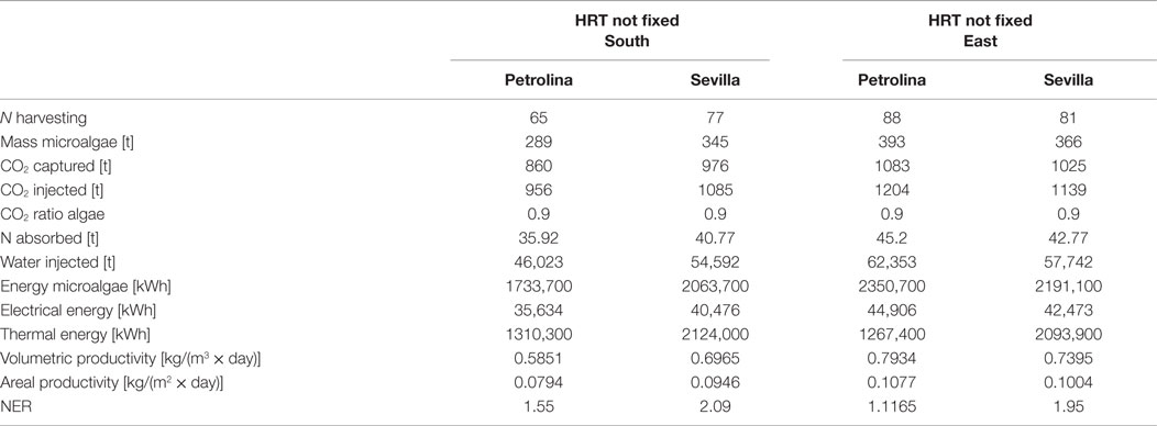
Table 8. Results from flat panel simulations using the first operating strategy, meaning that input and output microalgae concentrations are known.

TABLE 9

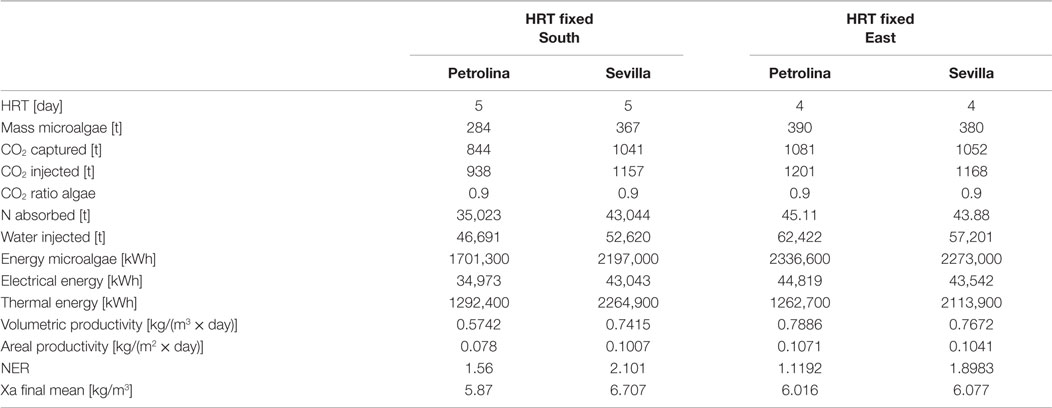
Table 9. Results from flat panel simulation using the second strategy, meaning that input microalgae concentration and HRT are known.

For the two operating strategies, results are reported for both the locations (Sevilla and Petrolina) and for the two most significant orientations, that is when the flat panel is facing south (and north) and when it is facing east (and west). The east–west orientation appears to be preferable in both locations because it leads to a higher microalgae production: as explained by Sierra et al. (2008), if the orientation of the two faces of the reactor is east–west, the intercepted radiation is maximum during the first and last solar hours, because of the orientations toward sunrise and sunset. Thus, light availability during the daylight solar cycle is also more homogenous for this configuration. Areal and volumetric productivities are consistent with those found in literature: Chisti (2007) reports a volumetric productivity equal to 1.535 kg m⁻³ day⁻¹, which is higher than the values obtained from the model; if compared to some other works, the results of the dynamic model, in particular the areal productivity, seem to be optimistic: for example, the microalgae production coming from the model [~400 t/(ha × year)] is two times higher than the production obtained by Slegers et al. (2011) from a flat panel reactor located in Algeria which produces up to 200 t/(ha × year). Moreover, the volumetric productivity for a flat panel reported by Jorquera et al. (2010) is equal to 0.27 kg m⁻³ day⁻¹, whereas the model supplies values equal to 0.8 kg m⁻³ day⁻¹. From a recent work by Münkel et al. (2013), volumetric productivities equal to 1.25 kg m⁻³ day⁻¹ have been reached in experimental analyzes. The difference from some values found in literature could be a consequence of a series of related factors: the microalgae species chosen may strongly influence the productivity of the reactor. Moreover, the model created in this work contains a temperature control, which fixes the temperature inside the reactor at the optimal level for microalgae growth: this means that the specific growth rate is not affected by the temperature factor (which is always equal to one), and consequently it is nearer to the maximum growth rate than in the real operating conditions. Furthermore, the locations chosen for the analysis present optimal values of irradiation, next to the saturation irradiation, where the light intensity factor affecting the growth rate is next to 1. From Tables 8 and 9 the high dependence on the orientation of the panel clearly appears in the productivity of Petrolina: if the two faces of the reactor are oriented toward east and west, the productivity is higher than in case of south and north orientation. A possible explanation might be related to radiation reflection by the panel: when the sun is high in the sky, the radiation hits the flat panel with an incidence angle close to 90°; if the incidence angle is too high, radiation could not enter the reactor, due to glass reflection. For this reason, if the panel is oriented toward south, the largest part of the radiation during summer is lost and does not contribute to microalgae growth: if the orientation if east–west, the radiation is collected during morning and afternoon with an incidence angle next to 0°. The same situation does not take place in Sevilla, because the sun does not reach high elevations during the whole year; the east–west orientation is preferable also in Sevilla, as suggested by Sierra et al. (2008).

In general, higher volumetric and areal productivity values have been reached both in Sevilla and in Petrolina, and the difference between the two locations is less remarkable than it was for the open pond; the flat panel photobioreactor growth model includes a temperature control, which maintains the temperature of the water at a constant level. In spite of the higher productivities, Sevilla appear to be less suitable for a flat panel photobioreactor than Petrolina, as shown by NER. The thermal energy requirement is extremely high in Sevilla, where winter time brings low atmospheric temperatures: the photobioreactor should operate only during summertime.

Microalgae mass production in flat panel reactor is much higher than in open raceway pond, CO₂ absorption is more efficient, but the thermal energy requirement implies a NER value >1. There are different possible strategies to solve this problem: keeping the water in the reactor within a range of suboptimal temperatures where the productivity of microalgae is still high and the thermal energy requirement is lower; leaving the temperature in the reactor without any control during the night: this might be an interesting solution also to limit the microalgae losses due to dark respiration, which are higher for optimal temperature. If water temperature is lower than the optimal value for growth, the metabolic energy required by the microalgae for their maintenance during the night is lower.

Discussion

Unlike the most common existing models in the literature, which deal with a specific part of the overall cultivation process, the models presented in this paper include all physical and chemical quantities that mostly affect microalgae growth. These features allow the model to correctly predict the overall behavior of microalgae cultivation plants for energy production. All input parameters can be tuned and varied to obtain reliable predictions.

This paper aims to present a model for microalgae cultivation where geometric and physical parameters, presented in recent works by Slegers et al. (2011, 2013), Duffie and Beckman (2013), Béchet et al. (2013) and more, receive a robust analysis together with the chemical and biological aspects, as presented by Yang (2011), Chisti (2007), Le et al. (2010), and more.

A comparison with experimental data taken from the literature shows that the predictions are consistent, only slightly overestimating the productivity in case of closed photobioreactor. The reason for the overestimation might be found in the temperature control strategy of the reactor, which is kept constant in the simulation runs. This strategy is currently applied in laboratory scale plants but it is expensive both from an economic and energetic point of you for a large scale cultivation plant.

The model is a part of a wider activity on microalgae cultivation plants for energy production which consider the additional directions of work:

- Further analysis could be conducted at the boundaries of the system taken into consideration by the model, evaluating and modeling the downstream microalgae transformation process and the upstream technologies that generate the input streams entering the cultivation phase.

- The cultivation phase model might be modified to include other less important, but still valuable parameters that influence microalgae growth, such as some other nutrients like phosphorus.

- The microalgae growth rate equation could be compared with other models in the literature and with results coming from real pilot plants to make predictions more reliable.

- The flat panel model should be tested with different temperature control strategies, which might lead to a lower productivity but also to a lower thermal energy consumption, making the technology more interesting from an economic point of view.

Conflict of Interest Statement

The authors declare that the research was conducted in the absence of any commercial or financial relationships that could be construed as a potential conflict of interest.

References

Ak, İ (2012). Effect of an organic fertilizer on growth of blue-green alga Spirulina platensis. Aquacult. Int. 20, 413–422. doi: 10.1007/s10499-011-9473-5

CrossRef Full Text | Google Scholar

Azadi, P., Brownbridge, G., Mosbach, S., Smallbone, A., Bhave, A., Inderwildi, O., et al. (2014). The carbon footprint and non-renewable energy demand of algae-derived biodiesel. Appl. Energy 113, 1632–1644. doi:10.1016/j.apenergy.2013.09.027

CrossRef Full Text | Google Scholar

Bahadar, A., and Bilal Khan, M. (2013). Progress in energy from microalgae: a review. Renew. Sustain. Energ. Rev. 27, 128–148. doi:10.1016/j.rser.2013.06.029

CrossRef Full Text | Google Scholar

Béchet, Q., Shilton, A., and Guieysse, B. (2013). Modeling the effects of light and temperature on algae growth: state of the art and critical assessment for productivity prediction during outdoor cultivation. Biotechnol. Adv. 31, 1648–1663. doi:10.1016/j.biotechadv.2013.08.014

PubMed Abstract | CrossRef Full Text | Google Scholar

Borowitzka, M. A. (1999). Commercial production of microalgae: ponds, tanks, tubes and fermenters. J. Biotechnol. 70, 313–321. doi:10.1016/S0168-1656(99)00083-8

CrossRef Full Text | Google Scholar

Brennan, L., and Owende, P. (2010). Biofuels from microalgae – a review of technologies for production, processing, and extractions of biofuels and co-products. Renew. Sustain. Energ. Rev. 14, 557–577. doi:10.1016/j.rser.2009.10.009

CrossRef Full Text | Google Scholar

Çelekli, A., and Yavuzatmaca, M. (2009). Predictive modeling of biomass production by Spirulina platensis as function of nitrate and NaCl concentrations. Bioresour. Technol. 100, 1847–1851. doi:10.1016/j.biortech.2008.09.042

PubMed Abstract | CrossRef Full Text | Google Scholar

Chisti, Y. (2007). Biodiesel from microalgae. Biotechnol. Adv. 25, 294–306. doi:10.1016/j.biotechadv.2007.02.001

PubMed Abstract | CrossRef Full Text | Google Scholar

Collet, P., Hélias, A., Lardon, L., Ras, M., Goy, R.-A., and Steyer, J.-P. (2011). Life-cycle assessment of microalgae culture coupled to biogas production. Bioresour. Technol. 102, 207–214. doi:10.1016/j.biortech.2010.06.154

PubMed Abstract | CrossRef Full Text | Google Scholar

Cuaresma, M., Janssen, M., Vílchez, C., and Wijffels, R. H. (2011). Horizontal or vertical photobioreactors? How to improve microalgae photosynthetic efficiency. Bioresour. Technol. 102, 5129–5137. doi:10.1016/j.biortech.2011.01.078

PubMed Abstract | CrossRef Full Text | Google Scholar

Davis, R., Aden, A., and Pienkos, P. T. (2011). Techno-economic analysis of autotrophic microalgae for fuel production. Appl. Energy 88, 3524–3531. doi:10.1016/j.apenergy.2011.04.018

CrossRef Full Text | Google Scholar

Doucha, J., and Lívanský, K. (2006). Productivity, CO2/O2 exchange and hydraulics in outdoor open high density microalgal (Chlorella sp.) photobioreactors operated in a Middle and Southern European climate. J. Appl. Phycol. 18, 811–826. doi:10.1007/s10811-006-9100-4

CrossRef Full Text | Google Scholar

Duffie, J. A., and Beckman, W. A. (2013). Solar Engineering of Thermal Processes, 4th edn. New York: A Wiley-Interscience Publication, John Wiley and Sons, Inc.

Google Scholar

Fernández, F. G. A., Camacho, F. G., Pérez, J. A. S., Sevilla, J. M. F., and Grima, E. M. (1997). A model for light distribution and average solar irradiance inside outdoor tubular photobioreactors for the microalgal mass culture. Biotechnol. Bioeng. 55, 701–714. doi:10.1002/(SICI)1097-0290(19970905)55:5

PubMed Abstract | CrossRef Full Text | Google Scholar

Fernández, F. G. A., Sevilla, J. M. F., and Grima, E. M. (2013). Photobioreactors for the production of microalgae. Rev. Environ. Sci. Biotechnol. 12, 131–151. doi:10.1007/s11157-012-9307-6

CrossRef Full Text | Google Scholar

Hadiyanto, H., Elmore, S., Van Gerven, T., and Stankiewicz, A. (2013). Hydrodynamic evaluations in high rate algae pond (HRAP) design. Chem. Eng. J. 217, 231–239. doi:10.1016/j.cej.2012.12.015

CrossRef Full Text | Google Scholar

Hempel, N., Petrick, I., and Behrendt, F. (2012). Biomass productivity and productivity of fatty acids and amino acids of microalgae strains as key characteristics of suitability for biodiesel production. J. Appl. Phycol. 24, 1407–1418. doi:10.1007/s10811-012-9795-3

PubMed Abstract | CrossRef Full Text | Google Scholar

James, S. C., and Boriah, V. (2010). Modeling algae growth in an open-channel raceway. J. Comput. Biol. 17, 895–906. doi:10.1089/cmb.2009.0078

PubMed Abstract | CrossRef Full Text | Google Scholar

Janssen, M., Tramper, J., Mur, L. R., and Wijffels, R. H. (2003). Enclosed outdoor photobioreactors: light regime, photosynthetic efficiency, scale-up, and future prospects. Biotechnol. Bioeng. 81, 193–210. doi:10.1002/bit.10468

PubMed Abstract | CrossRef Full Text | Google Scholar

Jiménez, C., Cossio, B. R., Labella, D., and Xavier Niell, F. (2003). The feasibility of industrial production of Spirulina (Arthrospira) in Southern Spain. Aquaculture 217, 179–190. doi:10.1016/S0044-8486(02)00118-7

CrossRef Full Text | Google Scholar

Jorquera, O., Kiperstok, A., Sales, E. A., Embiruçu, M., and Ghirardi, M. L. (2010). Comparative energy life-cycle analyses of microalgal biomass production in open ponds and photobioreactors. Bioresour. Technol. 101, 1406–1413. doi:10.1016/j.biortech.2009.09.038

PubMed Abstract | CrossRef Full Text | Google Scholar

Kochem, L. H., Da Fré, N. C., Redaelli, C., Rech, R., and Marcílio, N. R. (2014). Characterization of a novel flat-panel airlift photobioreactor with an internal heat exchanger. Chem. Eng. Technol. 37, 59–64. doi:10.1002/ceat.201300420

CrossRef Full Text | Google Scholar

Kumar, K., Dasgupta, C. N., Nayak, B., Lindblad, P., and Das, D. (2011). Development of suitable photobioreactors for CO2 sequestration addressing global warming using green algae and cyanobacteria. Bioresour. Technol. 102, 4945–4953. doi:10.1016/j.biortech.2011.01.054

PubMed Abstract | CrossRef Full Text | Google Scholar

Le, P. J., Williams, B., and Laurens, L. M. L. (2010). Microalgae as biodiesel & biomass feedstocks: review & analysis of the biochemistry, energetics & economics. Energy Environ. Sci. 3, 554–590. doi:10.1039/b924978h

CrossRef Full Text | Google Scholar

Mata, T. M., Martins, A. A., and Caetano, N. S. (2010). Microalgae for biodiesel production and other applications: a review. Renew. Sustain. Energ. Rev. 14, 217–232. doi:10.1016/j.rser.2009.07.020

CrossRef Full Text | Google Scholar

Molina, E., Fernández, J., Acién, F. G., and Chisti, Y. (2001). Tubular photobioreactor design for algal cultures. J. Biotechnol. 92, 113–131. doi:10.1016/S0168-1656(01)00353-4

PubMed Abstract | CrossRef Full Text | Google Scholar

Münkel, R., Schmid-Staiger, U., Werner, A., and Hirth, T. (2013). Optimization of outdoor cultivation in flat panel airlift reactors for lipid production by Chlorella vulgaris. Biotechnol. Bioeng. 110, 2882–2893. doi:10.1002/bit.24948

PubMed Abstract | CrossRef Full Text | Google Scholar

Muñoz, R., and Guieysse, B. (2006). Algal-bacterial processes for the treatment of hazardous contaminants: a review. Water Res. 40, 2799–2815. doi:10.1016/j.watres.2006.06.011

PubMed Abstract | CrossRef Full Text | Google Scholar

Norsker, N.-H., Barbosa, M. J., Vermuë, M. H., and Wijffels, R. H. (2011). Microalgal production – a close look at the economics. Biotechnol. Adv. 29, 24–27. doi:10.1016/j.biotechadv.2010.08.005

PubMed Abstract | CrossRef Full Text | Google Scholar

NREL, . (0000). Biomass Research – Publications. Available at: http://www.nrel.gov/biomass/publications.html?print

Google Scholar

Pruvost, J., Cornet, J. F., Goetz, V., and Legrand, J. (2011). Modeling dynamic functioning of rectangular photobioreactors in solar conditions. AIChE J. 57, 1947–1960. doi:10.1002/aic.12389

CrossRef Full Text | Google Scholar

Radmann, E. M., Reinehr, C. O., and Costa, J. A. V. (2007). Optimization of the repeated batch cultivation of microalga Spirulina platensis in open raceway ponds. Aquaculture 265, 118–126. doi:10.1016/j.aquaculture.2007.02.001

CrossRef Full Text | Google Scholar

Rawat, I., Ranjith Kumar, R., Mutanda, T., and Bux, F. (2013). Biodiesel from microalgae: a critical evaluation from laboratory to large scale production. Appl. Energy 103, 444–467. doi:10.1016/j.apenergy.2012.10.004

CrossRef Full Text | Google Scholar

Robinson, D., and Stone, A. (2004). Solar radiation modelling in the urban context. Solar Energy 77, 295–309. doi:10.1016/j.solener.2004.05.010

CrossRef Full Text | Google Scholar

Rodolfi, L., Chini Zittelli, G., Bassi, N., Padovani, G., Biondi, N., Bonini, G., et al. (2009). Microalgae for oil: strain selection, induction of lipid synthesis and outdoor mass cultivation in a low-cost photobioreactor. Biotechnol. Bioeng. 102, 100–112. doi:10.1002/bit.22033

PubMed Abstract | CrossRef Full Text | Google Scholar

Ruiz, J., Álvarez-Díaz, P. D., Arbib, Z., Garrido-Pérez, C., Barragán, J., and Perales, J. A. (2013). Performance of a flat panel reactor in the continuous culture of microalgae in urban wastewater: prediction from a batch experiment. Bioresour. Technol. 127, 456–463. doi:10.1016/j.biortech.2012.09.103

PubMed Abstract | CrossRef Full Text | Google Scholar

Sierra, E., Acién, F. G., Fernández, J. M., García, J. L., González, C., and Molina, E. (2008). Characterization of a flat plate photobioreactor for the production of microalgae. Chem. Eng. J. 138, 136–147. doi:10.1016/j.cej.2007.06.004

PubMed Abstract | CrossRef Full Text | Google Scholar

Sills, D. (2013). Modeling CO2 Requirements for Cultivation of Microalgae in Open Raceway Pond.

Google Scholar

Singh, N. K., and Dhar, D. W. (2011). Microalgae as second generation biofuel. A review. Agron. Sustain. Dev. 31, 605–629. doi:10.1007/s13593-011-0018-0

CrossRef Full Text | Google Scholar

Slegers, P. M., Lösing, M. B., Wijffels, R. H., van Straten, G., and van Boxtel, A. J. B. (2013). Scenario evaluation of open pond microalgae production. Algal. Res. 2, 358–368. doi:10.1016/j.biortech.2012.11.123

PubMed Abstract | CrossRef Full Text | Google Scholar

Slegers, P. M., Wijffels, R. H., van Straten, G., and van Boxtel, A. J. B. (2011). Design scenarios for flat panel photobioreactors. Appl. Energy 88, 3342–3353. doi:10.1016/j.apenergy.2010.12.037

CrossRef Full Text | Google Scholar

Sompech, K., Chisti, Y., and Srinophakun, T. (2012). Design of raceway ponds for producing microalgae. Biofuels 3, 387–397. doi:10.4155/bfs.12.39

CrossRef Full Text | Google Scholar

Stephenson, A. L., Kazamia, E., Dennis, J. S., Howe, C. J., Scott, S. A., and Smith, A. G. (2010). Life-cycle assessment of potential algal biodiesel production in the United Kingdom: a comparison of raceways and air-lift tubular bioreactors. Energy Fuels 24, 4062–4077. doi:10.1021/ef1003123

CrossRef Full Text | Google Scholar

Sugai-Guérios, M. H., Mariano, A. B., Vargas, J. V. C., de Lima Luz, L. F., and Mitchell, D. A. (2014). Mathematical model of the CO2 solubilisation reaction rates developed for the study of photobioreactors. Can. J. Chem. Eng. 92, 787–795. doi:10.1002/cjce.21937

CrossRef Full Text | Google Scholar

Sukhatme, K., and Sukhatme, S. P. (1996). Solar Energy: Principles of Thermal Collection and Storage. Noida, UP: Tata McGraw-Hill Education.

Google Scholar

Yang, A. (2011). Modeling and evaluation of CO2 supply and utilization in algal ponds. Ind. Eng. Chem. Res. 50, 11181–11192. doi:10.1021/ie200723w

CrossRef Full Text | Google Scholar

Appendix

Nomenclature

Asoil:	area of the pond that is embedded in the soil [m2]
Aw:	water surface area of the pond [m2]
CBowen:	Bowen constant [Pa/°C]
CO2D:	dissolved CO2 molar quantity in the bioreactor [mol/m3]
cpw:	heat capacity of the growth medium [J/(kg°C)]
CT:	total concentration of carbonate species in the bioreactor
d:	distance between the panels [m]
Eharv/refil:	electrical energy consumption for microalgae ­harvesting and reactor refilling [J]
$f_{\text{CO}}{}_2$:	flux of CO2 introduced by the supply of gas flow into the system [g/(m3 s)]
fI:	light intensity factor [−]
fT:	temperature factor [−]
g:	gravitational acceleration [m/s2]
Gdiffuse:	geometrical factor for diffuse radiation [−]
Gdirect:	geometric factor for direct radiation [−]
h:	height of the panels [m]
hcomb:	lower heating value on a dry basis of algae biomass [J/kg]
hshadow:	height of the shadow on the panel behind [m]
hsoil:	heat transfer coefficient of the surrounding soil layer [W/(m2°C)]
I0:	incident light intensity [W/m2]
Ia:	average light intensity in the volume of the bioreactor at a given time t [W/m2]
Iback:	radiation light intensity for the back surface [W/m2]
Idiffuse:	diffuse radiation over a horizontal surface [W/m2]
Idirect:	direct radiation over a horizontal surface [W/m2]
Ifront:	radiation light intensity for the front surface [W/m2]
IGHR:	global horizontal radiation [W/m2]
Is:	saturation light intensity for microalgae species [W/m2]
Isurface:	total light arriving on the pond [J/(kg°C)]
KC, KNA:	half-saturation constants [mol/m3]
Ke:	light extinction coefficient [m−1]
Ke1, Ke2:	light extinction constants
kLgα:	mass transfer coefficient for a given element
k1, k2:	carbonate species equilibrium constants
M:	concentration of the respective component [g/m3]
M*:	saturation concentration of the associated dissolved element [g/m3]
NT:	dissolved nitrogen molar quantity in the bioreactor [mol/m3]
PAR:	photosynthetic active radiation [%]
pa:	ambient pressure [Pa]
Ppump:	power of the installed pump for harvesting and refilling of the reactor [W]
pref:	reference pressure [Pa]
p′a:	water pressure of the air [Pa]
p′s:	saturated water pressure [Pa]
Q:	volumetric flow rate [m3/s]
Qalgae:	light energy flow to algae during growth [W]
Qcond:	heat flow between the pond and the ground via conduction [W]
Qconv:	heat flow by convection [W]
Qevap:	heat flow caused by either evaporation or condensation [W]
Qirr:	heat flow to the pond by sunlight [W]
Qrad:	heat flow by emission of long-wave radiation in the infrared region [W]
rgA:	microalgae growth rate [g/(m3 s)]
RH:	relative humidity [−]
Rp:	reflection coefficient for p-polarized light [−]
Rs:	reflection coefficient for s-polarized light [−]
R′:	overall reflection coefficient for each interface [−]
R′1:	overall reflection coefficient for the air – reactor ­interface [−]
R′2:	overall reflection coefficient for the reactor – culture interface [−]
s:	position in bioreactor depth [m]
Ta:	air temperature [°C]
Tdew:	dew point temperature [°C]
tharv/refil:	time for microalgae harvesting and reactor refilling [s]
Tlet:	lethal temperature for microalgae species [K]
Tm:	transparency of wall material [−]
Topt:	optimal temperature for microalgae species [K]
Tsky:	equivalent sky temperature for clear sky days [K]
Tsoil:	temperature of the soil surrounding the pond [°C]
tsolar:	number of hours after solar midnight [−]
Tw:	water temperature in the bioreactor [K]
Tw:	pond temperature [°C]
VR:	reactor volume [m3]
XA:	microalgae concentration in the bioreactor [g/m3]
y:	position in reactor height [m]
YAM:	mass of the respective component consumed or generated by the microalgae per unit mass of microalgae produced [gM/gmicroalgae]
z:	pond depth [m] or photobioreactor thickness [m]
β:	slope of the reactor [°]
βalgae:	curve modulating constant for the temperature fac it depends on microalgae species
γ:	azimuth angle [°]
ϵw:	emissivity of the water in the infrared region [−]
ηi:	refractive index of the material before the interface [−]
ηpump:	efficiency of the pump [−]
ηt:	refractive index of the material after the interface [−]
θ:	solar incidence angle [°]
θi:	incidence angle [°]
θz:	solar zenith angle [°]
μA:	microalgae specific growth rate [s−1]
${\widehat{\mu }}_{\text{A}}$:	maximum microalgae specific growth rate [s−1]
ρ:	water density [kg/m3]
ρw:	density of the growth medium [kg/m3]
σ:	light extinction coefficient [m]
σSB:	Stefan–Boltzmann constant [W/(m2K4)]