Optimal Operations and Resilient Investments in Steam Networks

1. Introduction

Steam is used as an energy carrier in industrial sites, converting heat into a usable energy source. Some of its major uses are process heating (heating at constant temperature), cogeneration of mechanical power (steam turbines), and stripping (direct injection of steam into a distillation column to improve distillation).

In industrial clusters, steam is produced in a centralized boiler house at high pressure, from which it can enter the steam headers of a steam network. Process units may consume steam at different pressure levels depending on the process requirements. Processes with high temperatures can also be cooled with pressurized water, producing steam.

Steam that is not consumed at a given pressure level can be cascaded to lower pressure headers through steam turbines (producing mechanical power) or through letdowns (isenthalpic expansion), often coupled to desuperheaters. Desuperheaters reduce the temperature of steam by injection of demineralized water, thereby increasing the steam flow.

In a well-regulated steam network, there should be no excess steam at the lowest pressure level. In the case of imbalance, the lowest pressure steam can either be condensed by a cooling utility or vented to the atmosphere. In both cases, heat is wasted, and in the latter case, costly demineralized water is lost.

Optimal operations of steam networks should aim to:

• Minimize the cost and environmental impacts of steam production by choosing appropriate steam producing equipments and fuels.

• Maximize the use of steam turbines to cogenerate power.

• Minimize venting of steam to the atmosphere.

• Maximize the condensate return.

• Activate the appropriate letdowns and desuperheaters when operating reserves are low (if demand is equal to the available steam production capacity, for example).

While these principles are trivial and often self-regulating, understanding the operations of a large steam network can quickly become challenging as the numerous equipments and processes consume and produce steam across several pressure levels.

Steam demand may be planned but is rarely constant. Irregular process unit consumption and production are the principal causes for its variations. Process units may incur exceptionally high demand during startups, when catalysts are aging or when certain steam producing process units go offline.

Weather can also contribute toward steam demand. In the cold winter months, increased steam tracing of pipes is required to prevent fluids from freezing. Heavy rains can cause floods, which leave steam pipes underwater, leading to thermal losses, and increased steam condensation in pipes. In both cases, boilers must produce more steam to satisfy the process heat requirements. Exceptionally, hot weather conditions can also affect demand, as exothermic process units may be forced to shutdown if cooling power is no longer available.

Boilerhouses are usually oversized to deal with high steam demand; however, situations can occur where demand surpasses the available steam production capacity and operating reserves fall to zero (undercapacity). This can happen when maintenance or boiler failures occur at the same time as high steam demand. In such cases, load shedding becomes the only solution to unsafe operations and even network failure.

Boilers are able to operate for extended periods of time if they are properly maintained. Maintenance operations can be planned ahead to minimize the disruptions to the steam supply. Despite regular maintenance, boiler failures can occur due to thermal or mechanical fatigue, corrosion, and overheating (Mcintyre, 2002). Boiler failures cannot be planned in advance and may need extensive periods of time for repair.

Resilience is defined as the ability of a system to respond to perturbations and to recover from them. In the case of a steam network, perturbations are mainly caused by extreme weather events, exceptional demand, boiler maintenance, and boiler failures. While the first three causes can be mitigated with proper planning, given the stochastic nature of boiler failures, the resilience of a system can be strongly affected by them.

Optimization works on steam studies have addressed optimal operations and investments using limited data sets; however, little has been done to establish the right amount of oversizing (and number of equipments to install) and the resilience of the network.

The novelty of this work is therefore to define a framework to establish the optimal operations and investments for steam networks as well as their resilience. Through a simulation of these failures combined to an analysis of key performance indicators the resilience of a system as well as oversizing requirements can be established.

1.1. Existing Work and Literature Review

Mixed Integer Linear Programing (MILP) formulations offer powerful tools to optimize the operations and investments of steam networks (Papoulias and Grossmann, 1983). When extended to multiperiod and to include unit start ups (Iyer and Grossmann, 1997), more accurate results can be achieved. This formulation can also be used to optimally choose between the use of letdowns and their desuperheaters or turbines to generate power (Bungener et al., 2015a).

Further improvements were made by using part load efficiencies for steam producing equipments (Varbanov et al., 2004; Voll et al., 2013) and Mixed Integer Non-Linear Programing (MINLP) formulations (Bruno et al., 1998; Chen and Lin, 2011) have produced more realistic results at the cost of higher computing power.

During the operation of a complex industrial site, undercapacity events occur when operating reserves fall to zero. In the case of electric networks, load shedding can be applied when operating reserves are low, with customers being forced to shutoff their demand to prevent system wide blackouts and equipment damage (Laghari et al., 2013). This concept can also be applied to steam networks (Bungener et al., 2015a) though no rigorous optimization procedure has yet been formulated.

Oversizing of steam producing equipments is common practice to maintain adequate levels of operating reserve in all situations. Systems should be sized to ensure operability when dealing with disruptive events, such as extreme demand or boiler maintenance and failures. Investment optimization studies (Papoulias and Grossmann, 1983; Iyer and Grossmann, 1997) have established the minimum size of an investment without indicating the size of a realistic investment to ensure operability. Properly oversizing a system implies choosing the right number of redundant equipments as well as their total sizes, a subject that has not been explored for steam networks.

Failures leading to equipment shutdowns are an inevitability in boilers (Mcintyre, 2002), often caused by mechanical or thermal stresses and corrosion (Bungener et al., 2015b). These have not been included in previous steam network optimization studies. While boiler maintenance can be considered in the sizing of a system, boiler failures have a stochastic nature, and therefore, require a different approach, such as scenario-based analysis or Monte-Carlo simulations.

The reliability of electric networks has been addressed through indicators, such as Loss of Load Probability (Schenk et al., 1984), to measure the likelihood of demand exceeding installed capacity over a period of time. This method cannot be transposed to steam networks due to the complicated interactions between pressure levels, turbines, letdowns, and desuperheaters, which must be modeled for each unit of time. In order to judge the reliability and resilience of an investment, indicators reflecting the operability of the steam network should therefore be developed.

1.2. Aim of the Work

While important work has been carried out on operations and investment optimization, load shedding as a means to avoid undercapacity has not been included in the operations and sizing of boilerhouses. Furthermore, understanding the impact of oversizing and the resilience of steam networks has yet to be addressed.

This work therefore aims to build upon existing work and introduce a formulation for load shedding into the operational and investment optimization of steam networks. A methodology to simulate boiler failures in a network and evaluate its resilience is then proposed. The major steps are the following:

1. Existing MILP formulations: this paper aims to study and adapt state of the art mathematical formulations to decide on the optimal operations of a steam network.

2. High temporal resolution application: previous works have taken into consideration multiple scenarios. This work includes entire yearly data sets of steam demand to calculate optimal operational costs and to size investments considering peak demand and extreme operating conditions.

3. Load shedding: load shedding is introduced into the MILP formulation to overcome undercapacity.

4. Optimally chosen and sized investments: a method for choosing the best investment and operating reserves of a steam network is proposed, including load shedding as an option in the design procedure.

5. Key performance indicators: several indicators to measure the steam network resilience are investigated.

6. Simulation of steam network operations: a novel method is proposed to simulate the optimal operation of steam networks considering random boiler failures.

The models and methods are demonstrated using a case study based on measured data of an industrial cluster, composed of two individual sites.

2. Steam Network Model

The proposed steam network model is formulated using mathematical programing techniques, based on the sets and variables. The formulations concerning operations and investment optimization are derived from Papoulias and Grossmann (1983) and Iyer and Grossmann (1997) and are rewritten for clarity. Decision variables are presented in bold while parameters are left in normal font.

2.1. Optimal Operations

The problem is formulated as an MILP, using variables, parameters, constraints, and an objective function to be minimized. The steam network model is defined by considering a set of consumers and producers that will use or produce steam at a given pressure level.

Equation (1) is a constraint which defines the flow rate F_n,t of unit n at time t by its minimum F_min,n,t and maximum F_max,n,t allowed values. The binary variable y_n,t defines if a unit or utility device such as a turbine or letdown is activated.

$F_{\mathit{min},n,t}\cdot {\mathbf{\text{y}}}_{\mathbf{\text{n}},\mathbf{\text{t}}}\le {\mathbf{\text{F}}}_{\mathbf{\text{n}},\mathbf{\text{t}}}\le F_{\mathit{max},n,t}\cdot {\mathbf{\text{y}}}_{\mathbf{\text{n}},\mathbf{\text{t}}}\forall n,t$ (1)

Equation (2) removes all degrees of freedom from process units q, effectively transforming them into a parameter of the problem, with fixed flow rates. The quality and quantity of steam delivered to process units are defined by their requirements in heat at a given temperature.

$F_{\mathbf{\text{min}},\mathbf{\text{q}},\mathbf{\text{t\hspace{0.17em}}}}=F_{\mathit{max},q,t}{\mathbf{\text{y}}}_{\mathbf{\text{q}},\mathbf{\text{t}}}=1\forall q,t$ (2)

Equation (3) defines the mass balance of each header h from which steam can be collected and distributed. Each unit belongs to a set of units entering (I_h) or exiting (O_h) a header.

${\displaystyle \sum _{n\in O_h}}{\mathbf{\text{F}}}_{\mathbf{\text{n}},\mathbf{\text{t}}}-{\displaystyle \sum _{n\in I_h}}{\mathbf{\text{F}}}_{\mathbf{\text{n}},\mathbf{\text{t}}}=0\forall n,t,h$ (3)

A process unit can consume steam in one header and produce in another and is defined as multiple units in this model. An additional constraint is therefore added to force the binary variables y_n,t of such units to have the same value.

A letdown is treated similarly to a header, with an inlet unit in set I_l and an outlet unit in set O_l. The outlet can be increased by a factor α, corresponding to the additional steam created through desuperheating using demineralized water. This factor is calculated using thermodynamic tables based on the temperature of superheated steam and the desired temperature at the outlet of the desuperheater.

${\displaystyle \sum _{n\in O_l}}{\mathbf{\text{F}}}_{\mathbf{\text{n}},\mathbf{\text{t}}}-{\displaystyle \sum _{n\in I_l}}{\mathbf{\text{F}}}_{\mathbf{\text{n}},\mathbf{\text{t}}}\left(1+{\mathrm{\alpha }}_l\right)=0\forall n,t,l$ (4)

In order to achieve a general formulation, cogeneration units are considered as boilers with electric production. Steam compressors can be considered as turbines, which consume electricity and increase the pressure level of steam. Through the use of sets, it is possible to define multiple independent steam networks.

The operational cost c_Op,n,t [equation (5)] of unit n at time t is the product of its flow rate by the fuel costs c_n,t (or other operational costs) from which its electric production can be subtracted. This electric production is quantified by the price of electricity e_t and specific work of the unit w_n, which should be calculated using thermodynamic calculations and based on nominal values.

${\mathbf{\text{c}}}_{\mathbf{\text{Op}},\mathbf{\text{n}},\mathbf{\text{t}}}=\left(c_{n,t}-e_t\cdot w_{n,t}\right)\cdot {\mathbf{\text{F}}}_{\mathbf{\text{n}},\mathbf{\text{t}}}\forall n,t$ (5)

2.2. Operations with Undercapacity and Load Shedding

Undercapcacity occurs when operating reserves are unable to meet remaining demand. In such a situation, load shedding is required to keep the network operational. Process units can be switched off one after the other to reduce demand and reach the operating reserve limit. The order of shutdowns is defined by operators, though some degrees of freedom may exist, for example, if two units are of equal operational importance. For this, it is necessary to introduce a penalty cost corresponding to the loss in earnings due to a process unit shutdown or reduced production operation. The penalty costs are the economic manifestation of disturbances to the system.

The units that can be switched off for load shedding are therefore no longer defined as process units [defined by equation (2)], but rather as a producers and consumers with free integer variables y_n,t.

Equation (6) is used when shedding priorities are defined by the operators. The equation acts on groups of units G_p,s of shedding order number p for each site s. It can deactivate the unit n that is in shedding order level p only if all the units in shedding order level p − 1 and lower have already been deactivated. Using this formulation, the optimizer may choose which unit of each group to deactivate first based on economic criteria.

${\mathbf{\text{y}}}_{\mathbf{\text{n}},\mathbf{\text{t}}}|n\in G_{p,s}\ge {\mathbf{\text{y}}}_{\mathbf{\text{n}},\mathbf{\text{t}}}|n\in G_{p-1,s}\ge \dots \ge {\mathbf{\text{y}}}_{\mathbf{\text{n}},\mathbf{\text{t}}}|n\in G_{1,s}\forall n,t,s,p$ (6)

Equation (7) assigns the penalty costs c_Pen,n,t associated with unit deactivation for unit n at time t. P_n is the penalty cost (or lost profit) associated with shutting off unit n for a time step.

${\mathbf{\text{c}}}_{\mathbf{\text{Pen}},\mathbf{\text{n}},\mathbf{\text{t}}}=\left(1-{\mathbf{\text{y}}}_{\mathbf{\text{n}},\mathbf{\text{t}}}\right)P_n\forall n,t$ (7)

From an optimization point of view, equation (7) is sufficient to decide which unit to deactivate. The decision will, however, rely on the proper definition of the value of P_n that could require very complex economical calculations. Equation (6) sets priorities that include engineering knowledge and operational constraints to simplify the decision-making process.

2.3. Optimal Investment

With the following formulation, it is possible to identify optimally sized investments to meet demand in the steam network. Investment options must be defined in the network architecture through their fixed I_fix,n and variable investment costs I_var,n. The equation (8) gives the binary variable y_n of a units overall use and its maximum flow rate F_n to identify the investment size.

$\begin{array}{lll}\hfill \begin{array}{rl}& {\mathbf{\text{y}}}_{\mathbf{\text{n}}}\ge {\mathbf{\text{y}}}_{\mathbf{\text{n}},\mathbf{\text{t}}}\forall n\\ & {\mathbf{\text{F}}}_{\mathbf{\text{n}}}\ge {\mathbf{\text{F}}}_{\mathbf{\text{n}},\mathbf{\text{t}}}\forall n\end{array}& & \hfill \text{(8)}\end{array}$

Equation (9) calculates the annualized investment costs associated with an equipment. If the equipment has not been selected by the optimization, its investment costs will be zero.

${\mathbf{\text{c}}}_{\mathbf{\text{Inv}},\mathbf{\text{n}}}=I_{\mathit{fix},n}\cdot {\mathbf{\text{y}}}_{\mathbf{\text{n}}}+I_{\mathit{var},n}\cdot {\mathbf{\text{F}}}_{\mathbf{\text{n}}}\forall n$ (9)

Using a linear formulation for the investment costs has the limitation of not taking into consideration economies of scale (Papoulias and Grossmann, 1983). Piecewise linearization would improve the quality of the results (Voll et al., 2013) but would require an additional dimension for each equipment and higher computational complexity.

The objective function is described in equation (10). In this way, the optimizer will choose among operations, load shedding, and investment. An economically optimal result may include a combination of investments and load shedding at peak demand. To permit such an optimization, the binary variables of shedable process units must be left free.

$\mathbf{\text{Obj}}=\min \mathrm{\sum }_n\left(\mathbf{\text{In}}{\mathbf{\text{v}}}_{\mathbf{\text{n}}}+\mathrm{\sum }_t{d}_t\cdot \left({\mathbf{\text{c}}}_{\mathbf{\text{Op}},\mathbf{\text{n}},\mathbf{\text{t}}}+{\mathbf{\text{c}}}_{\mathbf{\text{Pen}},\mathbf{\text{n}},\mathbf{\text{t}}}\right)\right)$ (10)

Oversizing of systems is key to ensure operability. Steam networks should be able to operate normally (or at least without severe impediment) even if boilers are undergoing boiler maintenance. To do this, the optimization can be run considering permutations of key equipments being offline to identify necessary investment sizes.

2.4. Simulation of Steam Network Operations

Boiler failures are an inevitability of steam networks. Though occasional, they have the potential to be very costly. While it is highly improbable that two boilers will fail at the same time, as boiler failures can last for extended periods of time, it is possible for multiple boiler failures to overlap. Combinatorial probabilities can be used to calculate the probability of independent random events occurring simultaneously or consecutively (Abramson and Moser, 1970). Applied to boilers, these concepts highlight the risk of simultaneous boiler trips.

Establishing the probability of boiler events occurring at a given time and how much undercapacity will follow would allow a risk analysis to be carried out. However, as the problem becomes combinatorial, it is difficult to establish what the extreme conditions are or their probabilities. A simulation (space exploration method) is therefore proposed to evaluate the network without having to calculate these properties.

This section proposes a methodology to calculate expected steam network operation costs by simulating boiler failures based on their properties (the failure rate defined by the mean time between failures and the failure duration). As a reminder, boiler failures lead to sub-optimal equipment selection (higher costs) and load shedding (penalty costs).

Figure 1 illustrates the problem based on the case study data. Seven independent boilers are considered, belonging to 3 individual sites (Site 1, Site 2, CB). Boiler failures have been randomly simulated based on their properties, shown in Figure 1A. A boiler failure at Site 2 is followed by a CB boiler failure only a few days later, leading to a reduction of boiler capacity of 260 t/h for 3 days, shown in Figure 1B. During a period of high demand, this could potentially lead to significant undercapacity.

FIGURE 1

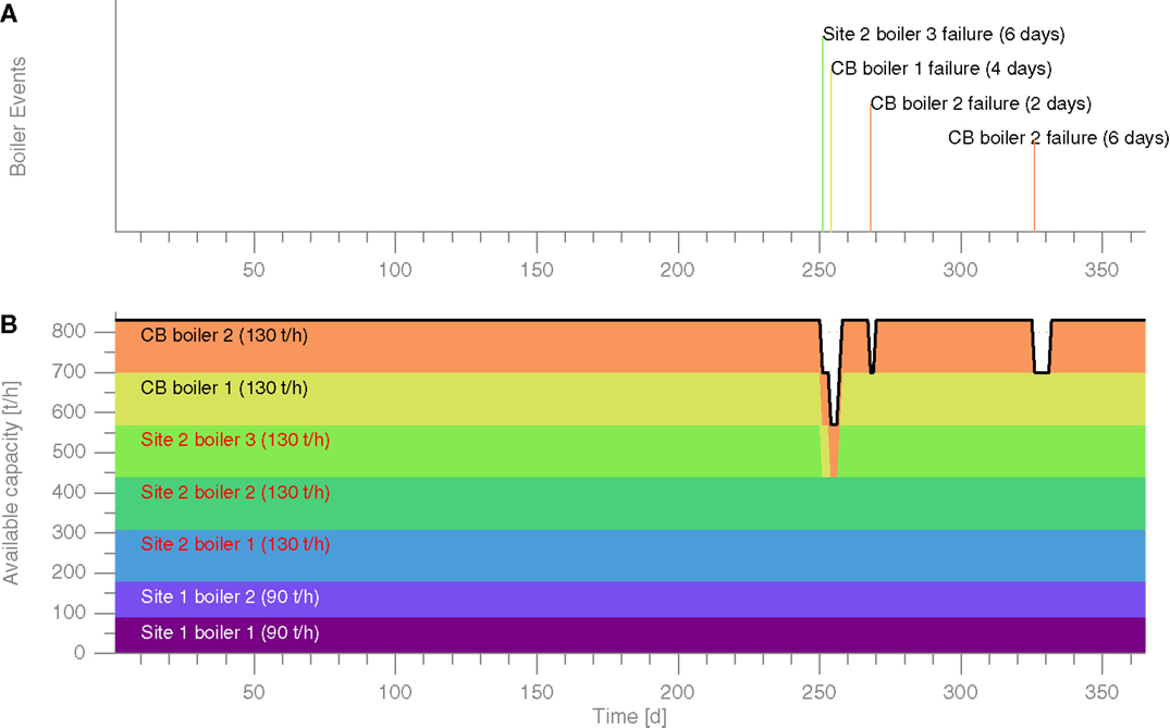
Figure 1. Simulated boiler failures. Random boiler trips (A) and resulting available steam generation capacity (B).

An algorithm is proposed to evaluate the resilience of a proposed investment as described below, illustrated step-by-step in Figure 2. It can be repeated for multiple investment proposals in order to compare them. Investments can be selected manually, or the proposed methodology for optimizing investment sizing can be used.

1. The network architecture, proposed investments, and data are input into the model.

2. Optimization of operations for a proposed investment: investments and operations are evaluated in design conditions using the operations optimization including load shedding to calculate design costs. No boiler failures are considered in this step.

3. Simulation of operations: a simulation is carried out by running m individual optimizations of the steam network.

(a) In each iteration Monte-Carlo sampling is used to randomly shutoff the boilers as described in equations (11) and (12) based on the mean failure rate (λ_b) and maximum failure duration (δ_b) of each boiler.

(b) The investment, operational and penalty costs as defined in equation (10) can be recorded for each iteration (Obj_m) as well as the investment configurations obtained and performance indicators.

(c) The simulation reaches convergence when both conditions in equation (13) are met, with σ_Obj the normalized SD of Obj_m (Ross, 2012).

4. Results are analyzed and key performance indicators are evaluated to establish the resilience and operability of the network.

FIGURE 2

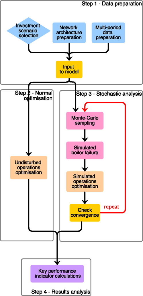
Figure 2. Simulated boiler failure algorithm.

Figure 1 was generated using the formulations in equations (11) and (12). A value x_b,t is randomly generated between 0 and 1 for each boiler and each time.

$\begin{array}{lll}\hfill \begin{array}{rl}& {\mathbf{\text{x}}}_{\mathbf{\text{b}},\mathbf{\text{t}}}=U\left(0,1\right)\forall b,t\\ & {\mathrm{\delta }}_{\mathbf{\text{b}},\mathbf{\text{t}}}=U\left(0,{\mathrm{\delta }}_b\right)\forall b,t\\ \end{array}& & \hfill \text{(11)}\end{array}$

If the value of the random number x_b,t is smaller than the boiler’s failure probability λ_b, its minimum and maximum flow rate are set to zero for a duration of time δ_b,t. This prevents boiler b from producing steam. δ_b,t is randomly chosen between 0 and δ_b, the maximum failure duration of boiler b.

$\text{if}{x}_{b,t}<{\mathrm{\lambda }}_b\left\{\begin{array}{cc}{\mathbf{\text{F}}}_{\mathbf{\text{max}},\mathbf{\text{b}},\mathbf{\text{t}}},\dots ,{\mathbf{\text{F}}}_{\mathbf{\text{max}},\mathbf{\text{b}},\mathbf{\text{t}}+\mathrm{\delta }}=0\hfill & \forall b,t\hfill \\ {\mathbf{\text{F}}}_{\mathbf{\text{min}},\mathbf{\text{b}},\mathbf{\text{t}}},\dots ,{\mathbf{\text{F}}}_{\mathbf{\text{min}},\mathbf{\text{b}},\mathbf{\text{t}}+\mathrm{\delta }}=0\hfill & \forall b,t\hfill \end{array}\right.$ (12)

$\text{Convergence\hspace{0.17em}when\hspace{0.17em}}\left\{\begin{array}{c}m>100\hfill \\ \frac{{\mathrm{\sigma }}_{\mathit{Obj}}}{\sqrt{m}}<\mathrm{\epsilon }\hfill \end{array}\right.$ (13)

Constant failure rates do not exist in reality, as failures depend upon the age of the equipment, the duration of time since the last failure, and a number of environmental parameters leading to increasing failure rates over time (Proschan, 1963). In our approach, the failure rate is calculated using equation (14) with the MBTF_b (Mean Time Between Failure of boiler b), obtained through observations of the case study boilers.

${\mathrm{\lambda }}_b=1∕\mathit{MBT}{F}_b$ (14)

Using variable failure, rates would imply knowing much more about the equipments under study and would add another dimension to the work. Similarly, we choose the failure duration randomly between 0 and the maximum failure duration of each boiler in equation (11). In reality, failures will last a certain amount of time based on the reason for failure.

2.5. Key Performance Indicators

As resilience is not a rigorous term, in this paper, it is quantified by studying economic- and operability-related indicators. Investment, operational, and penalty costs, and their simulated values reflect the expected economics of the network. Operability of the network is, however, a more novel concept; indicators are therefore introduced to quantify it.

2.5.1. Expected Costs

While the investment costs are constant for a given investment proposition, the operational and penalty costs may vary significantly depending on the disturbances. A statistical analysis on the total costs can therefore reveal important information. Box plots offer a way to visualize such information, with the mean, median, SD values, and outliers of the simulation results.

2.5.2. Operability

The term resilience is a general one. For this reason, the notion of operability is introduced as a measure of the expected frequency of shedding. The total number of recorded shedding events within a given optimization N_s is divided by the total number of binary decisions made about shedable units N_y and subtracted from one, equation (15).

For example, the case study is made up of 16 shedable units and utilities defined by 35 steam consumptions or productions (various pressure levels considered), with 365 time steps. The total number of binary decisions for shedable units is therefore N_y = 35 × 365 = 12,775. If 100 shedding events took place in a run, the operability would be 99.2%. An operability of 99.9% implies <13 shedding events in the entire cluster over a year.

$N=100\times \left(1-\frac{N_s}{N_y}\right)\left[-\right]$ (15)

The operability N of each iteration of the simulation can be calculated and generalizations can be made, namely,

• The expected operability $\overline{N}$ defined as the mean operability of each run.

• The operability interval: X_N the fraction of runs X which have an operability higher than Y. For example, if 95% of runs have an operability higher than 99.9 we have X_99.9 = 95%.

3. Case Study Description

For the case study, two adjoining industrial sites forming a cluster are considered. Site 1 is a refinery converting crude oil into fuels and feedstock for the petrochemical industry, whereas Site 2 is a petrochemical site producing a number of chemicals. All data and descriptions can be obtained from Bungener (2015). These data are for 365 days, using 24 h averages.

Both sites own and operate steam boilers to supply their process units and utilities (secondary operations, such as storage tank tracing and transport of fluids across the sites). Some process units also produce steam at various pressure levels. A third party owns two additional boilers connected to the high pressure steam headers of Sites 1 and 2. These will be referred to as the CB boilers (Central Boiler-house boilers).

Figure 3 illustrates the steam networks that are detailed below. Figure 4 shows the steam demand of both the sites using daily means over a year. Steam demand is equal to the difference between steam consumption and process unit steam production. To reach a high quality of data, an extensive work on data reconciliation is first carried out (Bungener et al., 2014), allowing for mass and energy balances to be closed (including unavoidable steam losses).

FIGURE 3

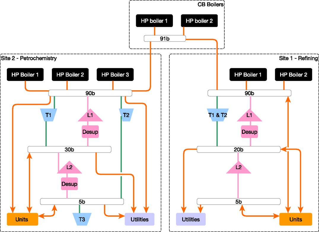
Figure 3. Architecture of steam networks of the industrial cluster.

FIGURE 4

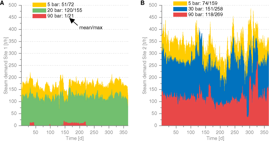
Figure 4. Steam demand of Site 1 (A) and Site 2 (B).

The shedding priorities and penalties of the sites’ units are included in the Table 1. The load shedding order corresponds to the order in which units can be shut off to deal with undercapacity. The penalty is the financial tax applied to the cost function when a unit is shed. Important units can be left as process units and not be allowed to shed at all given their critical nature.

TABLE 1

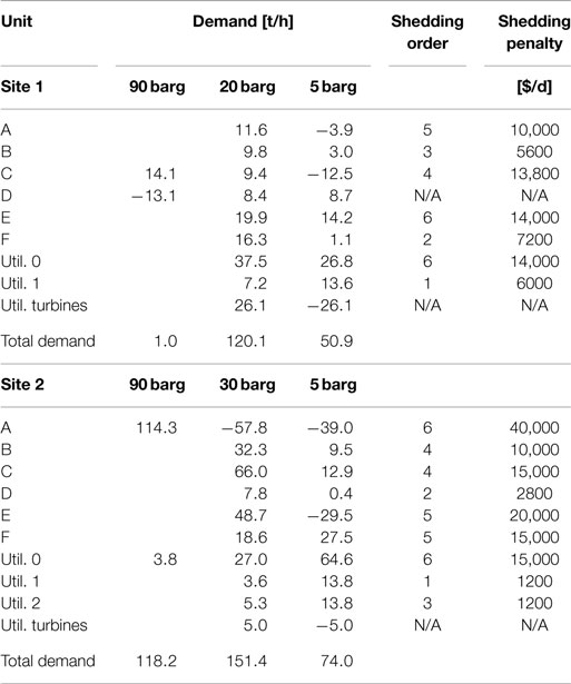
Table 1. Mean steam demand of Site 1 process units.

The terms F_min,n and F_max,n in Table 2, respectively, refer to the minimum and maximum flow rates of the steam producing equipments. The expected failure rate of a boiler p is the probability that it will shut down due to a failure, for a maximum duration d.

TABLE 2

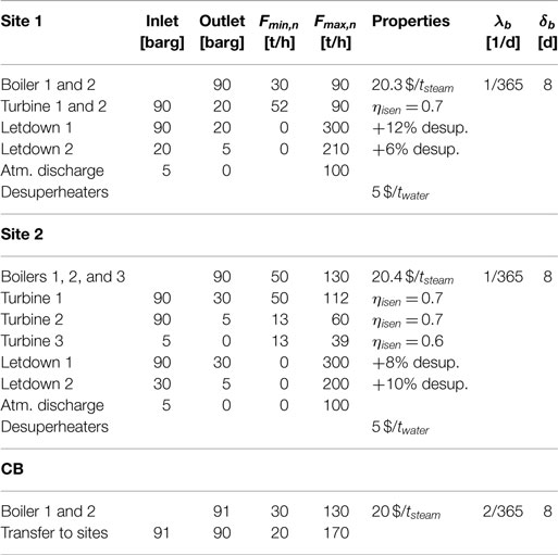
Table 2. Properties of site 1 boilers and steam network.

3.1. Site 1

The steam network of Site 1 is defined by its three pressure levels (90, 20, and 5 barg). Most of the steam demand takes place in the form of 20 barg steam. Two boilers produce 90 barg steam, which can then be distributed through two identical turbines from 90 to 20 barg or through a letdown coupled to a desuperheater. To transport steam from 20 to 5 barg, a letdown and a utility turbine exist. The utility turbine is set a process requirement given its critical nature.

Figure 4A shows the demand for steam throughout the year under study. The total steam demand has a mean of 172 t/h with a peak at 223 t/h. The peak 20 barg demand is 154.8 t/h compared to its mean 120.1 t/h. Globally, the steam demand for Site 1 is quite stable. Site 1’s demand surpasses 180 t/h (its installed boiler capacity) 33% of time. The peak demand takes place as a consequence of an extreme weather event.

3.2. Site 2

Site 2 has three pressure levels (90, 30, and 5 barg). Mean 90 barg steam demand is high at a mean 118.2 t/h. About 30 barg steam demand is also high with a mean of 151.4 t/h. Three boilers produce 90 barg steam, which can then be distributed through turbines to 30 or 5 barg. Letdowns coupled to desuperheaters can also expand the steam. The utility turbine can be considered as a process requirement.

Figure 4B shows the demand for steam throughout the year under study. The total steam demand has a mean value of 343 t/h with a peak at 487 t/h. The peak demand takes place as a consequence of combined high demand by several process units. The peak 90 barg demand is 269.2 t/h compared to its mean 118.2 t/h, caused by the startup of Unit A. The overall steam demand varies significantly during the year, surpassing its installed capacity (390 t/h) 13% of time.

3.3. CB Boilers

Two high pressure boilers make up the CB boilers, shown in Figure 3 and Table 2. Their steam can be sent to either sites through transfer lines. It should be noticed that the steam produced in the CB boilers is more costly as they are owned and operated by a third party. These boilers are considered to be old and nearing the end of their lifetime and are therefore subject to replacement in the case study.

3.4. Overall Demand

Figure 5B shows the load duration curves for the cluster (Sites 1 and 2 combined), corresponding to the demand curve ordered decreasingly with respect to the total demand. Figure 5A shows the installed steam production capacity of the cluster.

FIGURE 5

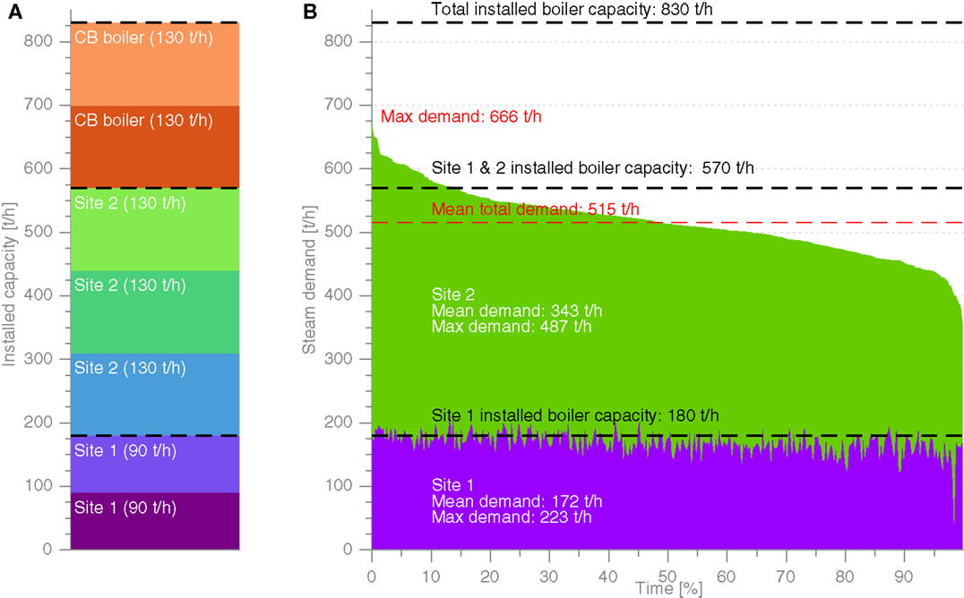
Figure 5. Cluster installed capacity (A) and load duration curve (B).

The load duration curves give indications as to the oversizing requirements of the cluster’s steam production capacity while also indicating important factors such as the peak and mean demands. These results also show the interest in industrial symbiosis by permitting sites to profit from each others’ operating reserves and the dependence of both sites on the CB boilers.

3.5. Proposed Investments

In the case study, considerations are made for the replacement of the CB boilers, which are at the end of their expected lifetime. Several investment options are considered, quantified by fixed I_fix and variable I_var investment costs. Table 3 summarizes the proposed investments and their annualized costs over 25 years.

TABLE 3

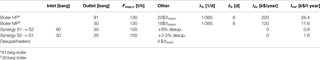
Table 3. Proposed investments to replace CB boilers.

Table 1 and Figure 4 show that most of the steam demand does not take place at 90 barg. For this reason, a 30 barg boiler (Boiler MP) is proposed for investment as well as a more expensive 90 barg boiler (Boiler HP). Up to three boilers of each type can be installed. No minimum flow rate F_min,n is defined for the proposed boilers.

Two synergy lines are also proposed in order to interconnect Site 1 (S1) and Site 2 (S2). These synergy lines offer the possibility to make use of the neighboring site’s excess steam at much cheaper cost than boilers. Both these lines are coupled to desuperheaters and a high shedding order (#1) to prevent steam sharing when operating reserves are low.

4. Case Study Optimization

First, the case study identifies the optimal operation of the steam network based on the existing configuration. Second, the old CB boilers are then removed from the optimization to demonstrate how to operate the network when facing undercapacity. Third, several investments propositions are made to replace the CB boilers. The network’s operations are then simulated using the proposed investments to compare them and conclude on their expected costs and resilience.

4.1. Optimized Operations with Current Configuration

Here, the optimal operations of the steam network are calculated. The total operational costs of the system are 79.5 × 10⁶$/year, the breakdown is shown in Figure 6. Electricity produced through cogeneration turbines is shown as negative costs. Desup refers to the cost of demineralized water when desuperheating is activated. Import refers to steam purchased from the CB boilers. These two generally activate at the same time.

FIGURE 6

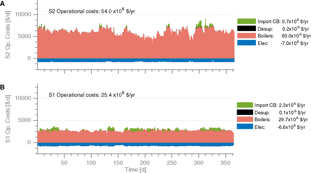
Figure 6. Economic results of steam network optimization under nominal operating conditions for Site 1 (A) and Site 2 (B).

Figure 7 summarizes the distribution of steam from the consumers to the producers. Import from the central boilers takes place only occasionally, when the demand is very high, with a peak of 96 t/h and a mean flow rate of 14 t/h. On the consumption side, Discharge corresponds to atmospheric venting, while the term Condensates refers to the activation of the condensing turbine in Site 2. These two tend to activate simultaneously signifying that Site 2 must be in excess of steam on several occasions.

FIGURE 7

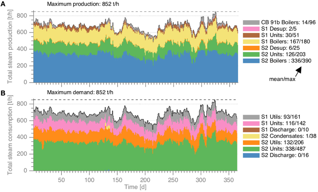
Figure 7. Steam distribution under nominal operating conditions for Site 1 (A) and Site 2 (B).

4.2. Load Shedding due to Offline CB Boilers

To demonstrate the effects of undercapacity as well as the way to deal with it, the CB boilers are removed from the steam network. The results are shown in Figure 8A, which shows the steam production and its inability to supply the total demand (red line), while Figure 8B shows which units are shed.

FIGURE 8

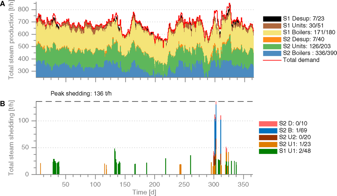
Figure 8. Overall cluster distribution of steam (A) and load shedding due to undercapacity (B).

The total costs are 86.9 × 10⁶$/year of which 7.1 × 10⁶$/year are penalties from process units being shut off. Given the inability to supply steam, the turbines are often shut off in favor of the letdowns and desuperheaters. This leads to increased operational costs (cost of demineralized water and loss of profit from electricity production).

In the worst case, process units are shed in both sites, totaling 136 t/h. A total of 72 shedding events take place, corresponding to an operability of N = 99.44%.

4.3. Investment Propositions

Here, the replacement solutions to the CB boilers are analyzed. Multiple options are considered so as to be able to compare investments.

1. Configuration 1: replacement of old CB boilers with two identical ones at the same pressure (130 t/h 91 barg boilers).

2. Configuration 2: minimum investment to permit operations under nominal operating conditions (no maintenance considered). This corresponds to investing in new common boilers for Sites 1 and 2 using the optimal investment formulation.

3. Configuration 3: minimum investment to permit operations with one boiler maintenance. The investment optimization is run considering a boiler offline in each site individually. The results are combined using the maximum-sized investment for each solution.

4. Configuration 4: minimum investment to permit simultaneous maintenance of two boilers, all year round. The investment optimization is run considering boilers offline at both sites simultaneously.

Configuration 1 is a simple replacement of the previous boilers. For Configurations 2–4, the formulation for optimal investment is used to determine the optimal size of boilers to be added.

The proposed equipments to invest in are described in Table 4. This corresponds to Step (2) of the algorithm illustrated in Figure 2.

TABLE 4

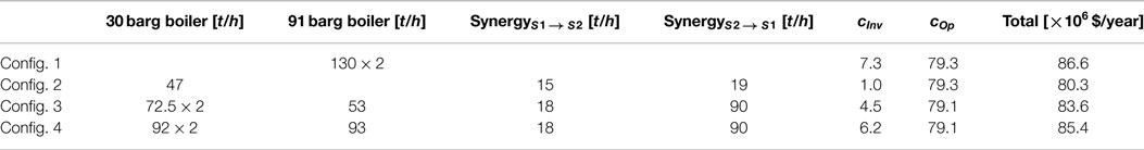
Table 4. Proposed investments to replace old CB boilers.

TABLE 5

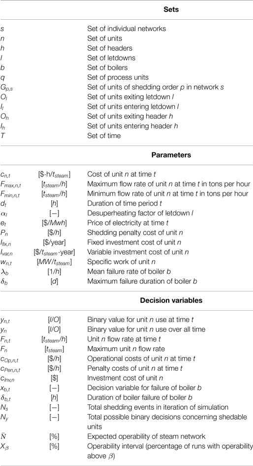
Table 5. Notations of sets, parameters, and variables.

Configuration 2 leads to the lowest investment costs. Configuration 1 leads to the highest investment costs. The lowest operational costs occur in Configurations 3 and 4, as the use of the synergy lines allows the sites to make use of each others cheaper steam rather than the more expensive steam from the new boilers.

4.4. Simulation of Operations for Proposed Investments

Using the identified investment configurations in Table 4, the steam network operations are simulated using the developed methodology [Step (3) of the algorithm]. The simulation is run for each configuration with ε = 3 × 10⁻³ as described in equation (13).

Figure 9 illustrates the results from the simulation of Configuration 3. In Figure 9A, we can see that the operational costs are very regular, though slight penalties can be applied from time to time. Figure 9B shows the peak shedding in each site, most of which comes from Site 2. Its key performance indicators are as follows [Step (4) of algorithm]:

• Mean simulated costs: 83.8 × 10⁶ $/year, slightly above the 83.6 × 10⁶ $/year design value.

• SD of costs: 0.3 × 10⁶ $/year SD can be attributed to load shedding and sub-optimal operations.

• Expected operability: $\overline{N}$ = 99.99%, equivalent to 1 shedding event per run on average.

• Operability interval: X_99.9 = 97.60% meaning that 97.6% of runs have an operability higher than 99.9%.

FIGURE 9

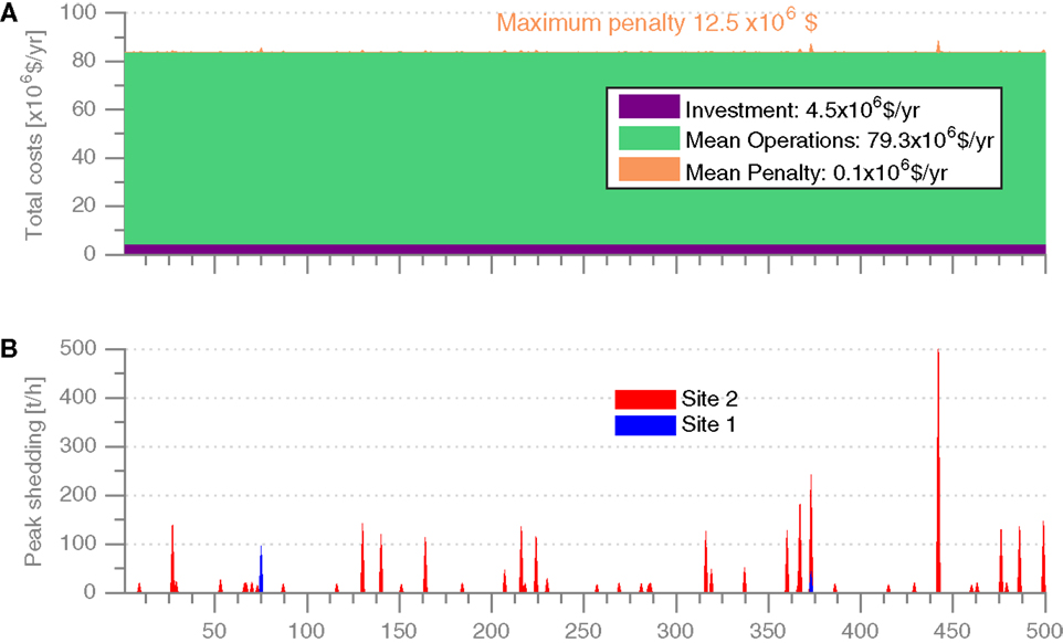
Figure 9. Simulation results for Configuration 2. Total costs (A) and peak load shedding (B).

The above analysis is repeated for each proposed investment in order to compare them. Figure 10 shows a comparative of the important results of the 4 simulations, sorted according to the mean simulated total costs. Figure 10A shows the mean economic results, while Figure 10B shows box plots to better understand the variability of each solution.

FIGURE 10

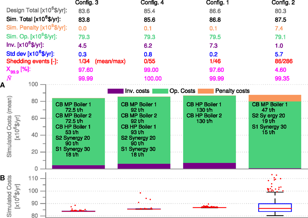
Figure 10. Comparison simulation results for each configuration. Expected costs (A) and variation analysis (B).

The results indicate that Configuration 2 provides the least resilient results as expected. Due to undersizing, a mean 86 shedding events take place per run, with a mean 7.4 × 10⁶ $/year in penalty costs. The box plot indicates that this configuration suffers from very high variability in costs with as much as 35 × 10⁶ $/year in costs overruns in worst case.

The operational costs of Configurations 1, 3, and 4 are similar and penalty costs are in general very small. These configurations are especially differentiated by their investment costs. The operability interval for Configuration 1 is lower than for Configurations 3 and 4. This result illustrates the advantage of installing the synergy lines between Sites 1 and 2 in order to give them access to each other’s steam.

The results indicate that Configuration 3 is the cheapest investment option while being highly resilient. The combination of small medium pressure boilers, high pressure boilers, and synergy lines leads to the lowest simulated overall costs and a small SD. The operability of the network remains very high despite boiler failures.

Configuration 3 may be the most attractive but is not necessarily the most resilient. From these results, we may only conclude that if no boiler maintenance is taking place, Configuration 3 is the most interesting. A sensitivity analysis on boiler maintenance would allow to better understand the risk and consequences associated with boiler failure.

The simulations of Configurations 1, 3, and 4 reached convergence criteria quickly, while Configuration 2 required 455 iterations. This can be explained by the spread of penalty costs obtained in Configuration 2, as seen in the box plots of Figure 10.

5. Discussion

The results have shown that a moderate investment including synergy lines between two industrial sites produced highly resilient results and the lowest expected costs. The cheapest investment configuration (no overcapacity) was much less resilient, leading to very high penalty costs. The high investment costs of the oversized solutions led to prohibitive total costs without necessarily offering increased operability.

Only 1 year of data was used in order to size the future system as it was assumed that enough variability was present within it to model any expected variability over the coming 25 years. While this assumption may be false, using more data would have been computationally challenging.

The use of variable failure rates would have brought more realism into the model and case study, though it would have difficult to implement given that only 1 year of data was used. To include variable failure rates, multiple data sets could be considered in an enlarged problem, with the failure rates increasing with time and resetting after a failure. This problem would, however, be very computationally heavy.

A sensitivity analysis on the parameters of the case study could provide important information about the potential drawbacks and benefits of certain solutions. However, given the scale of the problem, adding several more dimensions to it would have brought on significant computational and results analysis challenges, which may best be kept for future work.

Linear investment costs remain a weakness of this work, though through an iterative process, gross solutions can be fine-tuned with more appropriate costs until realistic investment results are reached.

The principal weakness of this method comes from the selection of the investment scenarios. To find optimally resilient investment solutions, a method is needed to generate configurations of equipments to invest in, to determine how much oversizing is necessary as well as the number of equipments to invest for the right amount of redundancy. A space exploration method such as Monte-Carlo sampling is unlikely to be efficient as the overall simulation time would become too long. The use of search heuristics such as an evolutionary algorithm could help find better solutions, especially since only one objective needs to be considered in the simulation.

6. Conclusion

This paper has built upon existing work on steam network optimization to include a load shedding formulation, which has in turn allowed for optimal operations to be established when facing undercapacity. Including load shedding into the investment formulation leads to the design of steam networks with the choice to invest for peak demand events, or to avoid high investments and apply load shedding to minimize costs.

A simulation of operations when facing unplanned boiler failures has allowed for calculations to be made on the resilience of the proposed investments, avoiding complex probabilistic studies to determine extreme events leading to undercapacity. Several key performance indicators were defined to judge the resilience of the investments.

A case study based on industrial data [made available online (Bungener, 2015)] has demonstrated the proposed methods and highlight the interest of oversizing systems and rethinking of existing solutions. Four investment scenarios were proposed to replace two boilers. The first scenario simply repeated a previous design of the system, while the other three used the optimized investment formulation to identify investment configurations while considering boiler maintenance simultaneously. Results showed the benefits of industrial symbiosis to maximize the use of existing equipments rather than investing in new ones.

The proposed methodology provides tools to optimize operations and determine the benefits of investment in boilers, cogeneration devices, or industrial symbiosis solutions. This method can also be applied at a smaller scale, for example, to determine the optimal operations of the steam network of a plant, and determine the interest in investments in its utility supply or even heat exchangers.

The development of a methodology to select optimally resilient investment configurations would significantly strengthen this work, though it remains an open research topic.

Author Contributions

SB: author; GE: co-director; and FM: director.

Conflict of Interest Statement

The authors declare that the research was conducted in the absence of any commercial or financial relationships that could be construed as a potential conflict of interest.

References

Abramson, M., and Moser, W. O. J. (1970). More Birthday Surprises, Vol. 77. Washington, DC: The American Mathematical Monthly, 856–858.

Google Scholar

Bruno, J. C., Fernandez, F., Castells, F., and Grossmann, I. E. (1998). A rigorous MINLP model for the optimal synthesis and operation of utility plants. Chem. Eng. Res. Des. 76, 246–258. doi: 10.1205/026387698524901

CrossRef Full Text | Google Scholar

Bungener, S. L. (2015). Data for Virtual Cluster. Available at: http://infoscience.epfl.ch/record/210192

Google Scholar

Bungener, S. L., Maréchal, F., and Van Eetvelde, G. (2014). “Modelling of a steam network using data reconciliation as a management tool,” in Energy Systems Conference (ENER) (London). Available at: http://infoscience.epfl.ch/record/209953

Google Scholar

Bungener, S. L., Maréchal, F., and Van Eetvelde, G. (2015a). Optimisation of Unit Investment and Load Shedding in a Steam Network Facing Undercapacity. 51329. Available at: www.sciencesconf.org

Google Scholar

Bungener, S. L., Descales, B., Van Eetvelde, G., and Maréchal, F. (2015b). Resilient decision making in steam network investments. Chem. Eng. Trans. 45, 73–78. doi:10.3303/CET1545013

CrossRef Full Text | Google Scholar

Chen, C.-L., and Lin, C.-Y. (2011). Design and optimization of steam distribution systems for steam power plants. Ind. Eng. Chem. Res. 50, 8097–8109. doi:10.1021/ie102059n

CrossRef Full Text | Google Scholar

Iyer, R. R., and Grossmann, I. E. (1997). Optimal multiperiod operational planning for utility systems. Comput. Chem. Eng. 21, 787–800. doi:10.1016/S0098-1354(96)00317-1

CrossRef Full Text | Google Scholar

Laghari, J. A., Mokhlis, H., Bakar, A. H. A., and Mohamad, H. (2013). Application of computational intelligence techniques for load shedding in power systems: a review. Energy Convers. Manag. 75, 130–140. doi:10.1016/j.enconman.2013.06.010

CrossRef Full Text | Google Scholar

Mcintyre, K. B. (2002). A review of the common causes of boiler failure in the sugar industry. Proc. S. Afr. Sug. Technol. Ass. 76, 355–364.

Google Scholar

Papoulias, S., and Grossmann, I. E. (1983). A structural optimization approach in process synthesis-II. Comput. Chem. Eng. 7, 707–721. doi:10.1016/0098-1354(83)85022-4

CrossRef Full Text | Google Scholar

Proschan, F. (1963). Theoretical explanation of observed decreasing failure rate. Technometrics 5, 375–383. doi:10.1080/00401706.1963.10490105

CrossRef Full Text | Google Scholar

Ross, S. M. (2012). Simulation. 5th Edn (Elsevier Science).

Google Scholar

Schenk, K. F., Misra, R. B., Vassos, S., and Wen, W. (1984). A new method for the evaluation of expected energy generation and loss of load probability. IEEE Trans. Power Appar. Syst. 103, 294–303. doi:10.1109/TPAS.1984.318228

CrossRef Full Text | Google Scholar

Varbanov, P. S., Doyle, S., and Smith, R. (2004). Modelling and optimization of utility systems. Chem. Eng. Res. Des. 82, 561–578. doi:10.1205/026387604323142603

CrossRef Full Text | Google Scholar

Voll, P., Klaffke, C., Hennen, M., and Bardow, A. (2013). Automated superstructure-based synthesis and optimization of distributed energy supply systems. Energy 50, 374–388. doi:10.1016/j.energy.2012.10.045

CrossRef Full Text | Google Scholar