Physics of the soil medium organization part 1: thermodynamic formulation of the pedostructure water retention and shrinkage curves

Introduction

The soil system, as it is actually considered in agro-environmental sciences, is represented as a vertical succession of horizontal layers defined as Representative Elementary Volumes (REVs) of the soil medium. This representation resulted in having similar and averaged hydrostructural properties of the soil medium. In this approach, all descriptive variables of the soil medium are average variables referenced to a volume (the REV) of which the internal organization, as well as its own delimitation, is ignored. It is obvious that no physical equation of these hydrostructural properties of the soil medium can be found if one ignores its internal organization; therefore, it is still a difficult task to define and describe any physical interaction between the water molecules and the solid particles making the structure (infrastructure) of this organization.

The use of the REV concept produced several empirical equations that are used in soil physics to characterize the hydro-physical properties of the soil medium, which imposes limitations upon the coupling of the soil physics with other agro-environmental disciplines (Ahuja et al., 2006). For example, the soil water retention curve [h(θ)] which links the volumetric water content (θ) [m³m⁻³ of soil] to the soil matrix pressure head (h) is still not physically determined and still represented by different parametric equations (El Kadi, 1985; Leij et al., 1997), showing that it is not coming from a unique theory of the soil medium organization. The case is the same with the other curves such as the hydraulic conductivity curve (Leij et al., 1997) and the soil shrinkage curve (Cornelis et al., 2006; Chertkov, 2012).

Braudeau and Mohtar (2009) proposed a new approach for characterizing and modeling the structured soil medium organization and its physical interaction with water. In this new approach, the basic concept of REV was replaced by the concept of Structural Representative Elementary Volume (SREV). This replacement was compulsory for defining a closed hydro-thermo-dynamic systems on the soil structure. Thus, in contrary to the REV, the SREV concept takes into account the soil structure and its hierarchy (Figure 1). Another complementary concept was used in the new approach, the pedostructure concept, which was proposed by Braudeau et al. (2004). Pedostructure concept defined and described the soil structure of a soil medium at its first level of organization as an assembly of primary peds and eventually inert mineral grains (sand). All the components present in a certain volume of the pedostructure are referred to the mass of the solid phase contained in this volume instead of being referred to the volume itself like in the REV concept (Figure 1). The change of REV to SREV leads to a completely different system of descriptive variables for the pedon and its internal organization like the horizons and pedostructures as mentioned in Table 1. Using this new system of variables the description of the pedostructure as an assembly of primary peds put in light the two complementary pore systems, said micro (intra primary peds) and macro (inter primary peds), of which the different hydrostructural behaviors are at the basis of all the soil water properties.

FIGURE 1

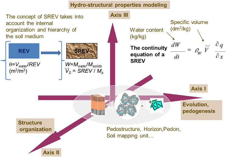
Figure 1. Fundamental difference between REV and SREV concepts after Braudeau and Mohtar (2009).

TABLE 1

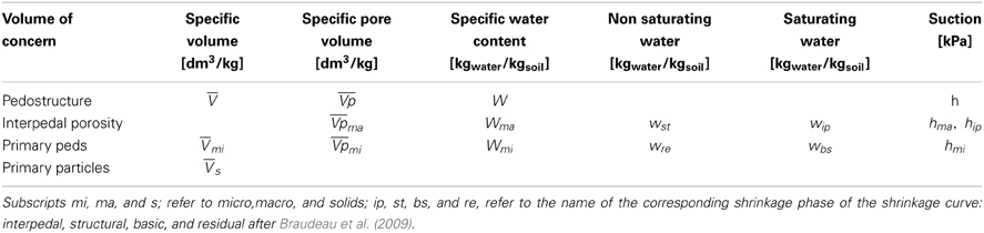
Table 1. Pedostructure state variables.

These two concepts, pedostructure and SREV, are at the basis of the new paradigm of hydrostructural pedology defining variables and physical units (Table 1) related to the pedon and its internal organization represented in Figure 2.

FIGURE 2

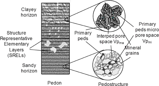
Figure 2. Representation of the internal organization of the pedon, hierarchized into its hydro-functional levels of organization: horizons, pedostructure, primary peds after Braudeau et al. (2009).

The computer model, Kamel^® (Braudeau et al., 2009) can be considered as representative of the generated new discipline, highlighting the following two key points:

  • The SREV concept and its system of specific variables, extensive and intensive, replaced the REV concept and its system of normalized volumetric variables (densities, water contents in m³/m³). Then, it was used for the description and simulation of all dynamic processes inside the pedon.

  • The distinction of the pedostructure water content (W) into W_mi and W_ma, as micro and macro water contents of the pedostructure, located respectively inside and outside of the plasmic porosity of primary peds.

In this article, and continuing to build on the two key points above, the authors wanted to apply the SREV concept to the thermodynamic theory of soil water written by Sposito (1981) based on the REV concept (hypothesis of homogeneous mixture of a tri-phasic “solids, water, air” soil medium). Therefore, this paper presents a new formulation of the thermodynamic functions and state equations of the soil medium, represented by its pedostructure. In particular, the thermodynamic formulation of the micro and macro pedostructure water contents at equilibrium [W^eq_ma(W) and W^eq_mi(W)], i.e., at equality of water potentials inside and outside of the primary peds at each equilibrium step of water removal from the pedostructure. The theory is presented hereafter establishing the generalized equations for the soil water retention curve h(W) and the shrinkage curve V(W). These equations will be validated in laboratory and compared with the previous equations proposed by Braudeau and Mohtar (2004, 2009), according to the pedostructure concept but without the notions of thermodynamic equilibrium of the soil medium.

Theory

Highlighting the Two Types of Water, Intra and Inter Primary Peds, in the Soil Medium

The distinction between internal and external water of the micro particles of a soil sample (W_mi and W_ma) was first quantitatively established by Braudeau (1988) from the interpretation of the soil shrinkage curve. In such testing, the shrinkage curve was continuously measured on soil samples of approximately 100 cm³ using very sensitive displacement sensors. This distinction of the water content (W) into both deformable micro- and macro-pore systems was quantitatively formulated assuming that the air entry point in the micropore system (primary peds) of the soil, separating de facto both nested micro and macro systems, can be accurately read from the measured shrinkage curve at the end of the basic shrinkage phase corresponding to the point B on the curve (Figure 3). This was confirmed by mercury porosimetry measurements (Braudeau and Bruand, 1993). In fact, this air entry point delineates conceptually and quantitatively the two nested pore systems: the micro pore system, that of the plasma composing primary peds, and the interpedal macro pore system at the surface outside of the primary peds and complementary to them in the pedostructure system volume (Figure 3, Table 1).

FIGURE 3

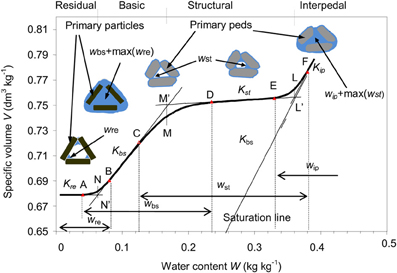
Figure 3. Various configurations of air and water partitioning into the two pore systems, inter and intra primary peds, related to the shrinkage phases of a standard Shrinkage Curve [water content vs. specific volume]. The various water pools [wre, wbs, wst, and wip] are represented with their domain of variations. The linear and curvilinear shrinkage phases are delimited by the transition points (A–F). Points N', M', and L' are the intersection points of the tangents at those linear phases of the Shrinkage Curve. Adapted from Braudeau et al. (2004).

Two formulations have been given to these types of water at equilibrium in terms of water content (W): an empirical formulation that resulted in an excellent fit with observed shrinkage curves [V(W)] (Braudeau, 1988; Braudeau and Bruand, 1993; Braudeau et al., 1999; Boivin et al., 2004; Boivin, 2007). Then, a physical formulation that based on a probabilistic reasoning by simultaneously removing those two types of water from both systems of the pedostructure during evaporation (Braudeau et al., 2004), such that:

$\begin{array}{cc}\begin{array}{l}{W}_{ma}=-\left(1/k_M\right)\text{Ln}\text{}\left(1+\exp \text{}\left(\text{-}{k}_M\text{}\left(W-W_M\right)\right)\right)\\ \text{with}{k}_M<0;\end{array}& (1\text{a})\end{array}$

and

$\begin{array}{cc}\begin{array}{l}{W}_{mi}=W-W_{ma}\\ =W+\left(1/k_M\right)\text{Ln}\text{}\left(1+\exp \text{}\left(-k_M\text{}\left(W-W_M\right)\right)\right)\end{array}& (1\text{b})\end{array}$

In these equations: W_mi and W_ma are considered complementary in the pedostructure specific pore volume Vp. While, the pedostructure parameters: k_M and W_M are characteristics of the hydro-structural behavior of the soil medium within the range of the shrinkage curve between the structural and the basic shrinkage phases, of slope K_st and K_ip, respectively (Figure 3). Hence, according to (1a) and (1b), W_M is equal in value to the maximum value of W_mi, i.e., W_miSat, and k_M is such that k_M = −Ln(2)/W_maM; they are parameters related to the sense and extension of the curvature near point M of the shrinkage curve on Figure 3. These parameters can be determined by fitting Equation (1) on the corresponding shrinkage range of the shrinkage curve which, on the other hand, should be continuously measured on soil samples according the methodology of Braudeau et al. (1999).

Then, in the study the soil water retention curve, h(W), associated to the shrinkage curve, V(W), of a soil sample using the device shown on Figure 4; Braudeau and Mohtar (2004) assumed that h(W) was directly linked to the macropore water content and is, in fact, governed by W_ma instead of W. They rewrote different equations of h(W) proposed in the literature, but in terms of W_ma rather than W according to the pedostructure concept. The equations tested were physically established by their authors (Berezin et al., 1983; Low, 1987; Rieu and Sposito, 1991) on the basis of different hypotheses made about the hydro-structural properties of the soil medium (fractal and thermodynamic) compatible to the pedostructure terminology (variables and parameters). Among them, the thermodynamic equation of Berezin et al. (1983), was modified into:

$\begin{array}{cc}{h}_{ma}={\rho }_w{\overline{E}}_{ma}\left(1/\left(W_{ma}+\sigma \right)-1/\left(W_{maSat}+\sigma \right)\right)& (2\text{a})\end{array}$

$\begin{array}{cc}{h}_{mi}={\rho }_w{\overline{E}}_{mi}\left(1/\left(W_{mi}-w_{re}\right)-1/\left(W_{miSat}-W_N\right)\right)& (2\text{b})\end{array}$

where h_mi and h_ma are positive and expressed in (kPa); E_mi and E_ma were defined as the potential energies of the solid phase resulting from the external surface charge of clay particles, inside and outside the primary peds, in (Jkg⁻¹ of solids); σ was defined as a part of the micropore water at interface with interpedal water in (kg water kg⁻¹ soil); w_re is the residual water content in (kg water kg⁻¹ soil), complementary of the basic water content w_bs in W_mi (Table 1) and defined by the interpretation of the shrinkage curve as shown in Braudeau et al. (2004). The terms: σ, w_re and W_N = w_reSat in Equation (2b) are pools of water added by Braudeau and Mohtar (2004) to take into account the air entry in the plasmic medium of primary peds.

FIGURE 4

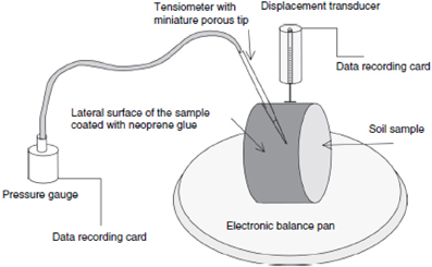
Figure 4. Device used by Braudeau and Mohtar (2004) for the simultaneous measurement of the soil water retention and soil shrinkage curves of a cylindrical soil sample.

The fitting results of observed shrinkage and water retention curves as measured in Braudeau and Mohtar (2004) using the device shown on Figure 4 and the calculated ones based on Equations (1) and (2) were good enough to confirm that W_ma is a control variable for these curves, including the shrinkage curve.

However, it was impossible at that time to give any information about h_mi(W_mi), the equilibrium relationship between h_mi and h_ma, as well as the validity of Equation (2) out of the tensiometer validity range, and other related questions like: the nature of the micro air entry point, the impact on the formulation of the curve, the need or not of parameters σ, and W_N in Equations (2a) and (2b). All these questions will be clarified in the present article. In fact, the challenge is now to introduce the thermodynamic theory, through the SREV concept, into the soil water physics already placed in the frame of the hydrostructural pedology.

Thermodynamic Formulation of W_ma and W_mi at Equilibrium State of the Pedostructure

Definition of the hydro-thermodynamic system of the soil medium

Applying the thermodynamic principles to the soil medium such that it can be considered as a physical and organized thermodynamic system exchanging material, liquid, gas, heat, and space with all other systems in contact with it, requires first the acknowledgment of the pedostructure as a thermodynamic system. The SREV concept defined by Braudeau and Mohtar (2009) transforms the virtual delimitation of any representative volume (REV) of the soil medium organization into a hydrostructural functional delimitation of this REV. Then, a SREV can be considered as a thermodynamic system closed on the mass of the solid phase of the structure (structural mass) contained in the delimited volume and cut by the delimitation bearing on the external parts of the structure enclosed. Accordingly, the structural mass of a SREV stays constant and can be taken as a reference, instead of the volume, for defining all the extensive variables describing its internal organization.

Thermodynamics variables of the soil medium organization

The definitive change brought by the SREV approach is that the descriptive variables of the internal organization of the soil can all be defined according to the hydro-structural and thermodynamics point of view. Table 1 lists the thermodynamic variables that describe the hydrostructural state of the soil organization at the pedostructure level of organization while Figure 2 shows the different hydro-functional levels of organization of the pedon, namely, the horizon, pedostructure SREV, primary peds and primary particles. There are two kinds of variables: intensive variables (temperature, pressure and water potential) and specific extensive variables (specific entropy, specific volumes, water and air gravimetric contents) which are extensive variables of the SREV reported to the same mass of reference, M_s: the structural mass of the considered SREV. Thus, all extensive variables of the pedostructure system are referenced to the mass of the solids (M_s) that compose the structure (the oven-dry mass of the pedostructure sample), such that V = V/M_s, A = A/M_s, etc. (Table 1). We will use the term of pedostructural instead of specific to qualify these variables reported to the mass of the pedostructure SREV. These definitions lead to the following relationships between the extensive variables:

$\begin{array}{cc}\overline{V}=\overline{Vp}+{\overline{V}}_S=W/{\rho }_w+\overline{A}/{\rho }_a+{\overline{V}}_s& (3\text{a})\end{array}$

$\begin{array}{cc}\begin{array}{l}W=W_{mi}+W_{ma},\overline{A}={\overline{A}}_{mi}+{\overline{A}}_{ma},\text{and}\\ \overline{Vp}={\overline{Vp}}_{mi}+{\overline{Vp}}_{ma}\end{array}& (3\text{b})\end{array}$

$\begin{array}{cc}{\overline{Vp}}_{mi}=\left(W_{mi}+{\overline{A}}_{mi}\right)/{\rho }_w\text{and}{\overline{Vp}}_{ma}=\left(W_{ma}+{\overline{A}}_{ma}\right)/{\rho }_w& (3\text{c})\end{array}$

where V, Vp, W, and A, are, respectively, the apparent pedostructural volume (dm³kg⁻¹) of soil, its total poral volume (dm³kg⁻¹), water mass content (kg_water kg⁻¹_solids), and air mass content (kg_air kg⁻¹_solids); V_s is the pedostructural volume of solid particles of soil (V_s = 1/ρ_s = V_s/M_s); ρ_s, ρ_w, and ρ_a being the densities of the structural solid particles, the water and air phases of the pedostructure in (kg dm⁻³), respectively. Subscripts mi, ma, w, and s refer to as micro, macro, water, and solids making the soil structure.

Practically, the classic undisturbed soil sample brought to the laboratory for physical analysis (in general a cylinder of about 5 cm diameter, 5 cm high sampled in a soil horizon) can be considered as a SREV of the soil medium of the soil horizon where it was sampled. The hydrostructural characteristics that will be measured on this sample in the laboratory are theoretically those of the soil medium in situ, in the corresponding horizon in the field. This makes it possible now to apply the thermodynamic principles to the physical description of the internal organization of the pedon in situ.

Thermodynamics of the pedostructure, basic concepts, and terminologies

To apply the pedostructure and SREV concepts to the “thermodynamic theory of water in soil” presented by Sposito (1981) according to the REV concept, we rewrote equations of the thermodynamic potentials U and G, the internal energy and the Gibbs energy, and their differential formulation, in such manner that: (i) the extensive variables (including the thermodynamic potentials themselves) are all reported to (divided by) the structural mass, M_s, of the pedostructure considered (a SREV of the soil medium organization); (ii) the two types of water W_mi and W_ma have been considered as two different components of the liquid water phase (W = W_ma + W_mi); (iii) the pedostructure at water saturation is the moisture state of reference for the soil water retention h (or soil water pressure) which is written h = −ρ_w(μ_w − μ_wSat), in kPa, with the water density ρ_w in kg/dm³; and iv) the chemical potentials: μ_w and μ_air of the water and air components, in Jkg⁻¹, are accounted negatively by convention. Then, the total differential of the specific internal energy U of a pedostructure SREV can be written such as:

$\begin{array}{cc}d\overline{U}=Td\overline{S}-Pd\overline{V}+{\mu }_{wma}d{W}_{ma}+{\mu }_{wmi}d{W}_{mi}+{\mu }_{air}d{\overline{A}}_{air}& (4)\end{array}$

where U is the specific internal energy (Jkg⁻¹_soil), S the specific entropy (JK⁻¹ kg⁻¹_soil), which are, like the other extensive variables of the SREV (Table 1), reported to the same structural mass M_s (the mass of solids making the structure of the considered SREV). As for the intensive variables, T is the absolute temperature (K), P is the external pressure (kPa), μ_wma and μ_wmi are the chemical potentials of the water inside and outside of primary peds (Jkg⁻¹_water) in the pedostructure.

In the usual terminology, the internal energy of a soil is a thermodynamic potential function U of which the independent variables are S, V, and {m_iα} which is a set of component masses, i indexing a component and α a phase in the soil medium (Sposito, 1981). As the other thermodynamic potentials obtained by performing the partial Legendre transformation on the internal energy U = U (S, V, {m_iα}), one can consider G as an extensive quantity that is equivalent in all respects to the internal energy U but controlled by the independent variables of state: T, P, and {m_iα}. “A knowledge of a thermodynamic potential is the same as a complete thermodynamic description of a soil” thus we can use U or G according to the set of controlled variables. Note that according to Sposito (1981): U = U/M_s = U (S, V, {m_iα/M_s}) or G = G/M_s = G (T, P, {m_iα/M_s}) are equivalent to U or G in terms of thermodynamic potential; however, the advantage of using the specific thermodynamic potentials U and G, expressed in units of joule by kg of soil structure, instead of U and G is to allow taking M_s, the mass of solids composing the structure of the SREV, as a reference for all organizational variables of this volume, including the pedostructural volume V. Thus, considering G as a positive extensive variable, the total differential of the specific free energy G of the pedostructure corresponding to dU should be written such as:

$\begin{array}{cc}d\overline{G}=\overline{S}dT-\overline{V}dP-{\mu }_{wma}d{W}_{ma}-{\mu }_{wmi}d{W}_{mi}-{\mu }_{air}d{\overline{A}}_{air}& (5)\end{array}$

and we can say that the hydrostructural and thermodynamic equilibrium of the soil medium is determined at U or G minimum, i.e., dU or dG = 0.

On the other hand, the Euler equation for G as an extensive variable is, according to Sposito (1981) (except for the sign):

$\begin{array}{cc}\overline{G}=-\left[{\displaystyle \sum _{\alpha }{\displaystyle \sum _i\left({\mu }_{i\alpha }-{\mu }_{i\alpha }^o\right)m_{i\alpha }}}\right]/M_S& (6)\end{array}$

where α represents the phase (solid, liquid, gaz), i the components in the considered phase, and μ^o_iα chemical potential of the chemical element under Standard State conditions. Subscripts str, wl, air in the following equations refer to as the solid, liquid and gaz phases in the pedostructure.

In the case of the pedostructure system (SREV), Equation (6) becomes:

$\begin{array}{cc}\overline{G}={\overline{G}}_{str}+{\overline{G}}_{wl}+{\overline{G}}_{air}& (7)\end{array}$

where

$\begin{array}{cc}{\overline{G}}_{str}=-{\displaystyle \sum _i\left({\mu }_{ist}-{\mu }_{ist}^o\right)}{m}_{ist}/{\displaystyle \sum _i{m}_{ist}}& (7\text{a})\end{array}$

$\begin{array}{cc}\begin{array}{l}{\overline{G}}_{wl}=-\left({\mu }_{wmi}-{\mu }_w^o\right)W_{mi}-\left({\mu }_{wma}-{\mu }_w^o\right)W_{ma}\\ ={\overline{G}}_{wmi}+{\overline{G}}_{wma}\end{array}& (7\text{b})\end{array}$

$\begin{array}{cc}{\overline{G}}_{air}=\left({\mu }_{air}-{\mu }_{air}^o\right)\overline{A}& (7\text{c})\end{array}$

The second law of the thermodynamics says that at equilibrium G is minimum and dG_α = 0 for all phases. Hence, for liquid phase in particular, one can write the following relations:

$\begin{array}{cc}d{\overline{G}}_{wl}=d{\overline{G}}_{wmi}+d{\overline{G}}_{wma}=0& (8)\end{array}$

$\begin{array}{cc}\begin{array}{l}d{\overline{G}}_{wl}=-d\text{}\left[W_{mi}\text{}\left({\mu }_{wmi}-{\mu }_w^o\right)\right]\\ -d\text{}\left[W_{ma}\text{}\left({\mu }_{wma}\text{-}{\mu }_w^o\right)\right]=0\end{array}& (9)\end{array}$

$\begin{array}{cc}\begin{array}{l}d{\overline{G}}_{wl}=-W_{mi}d{\mu }_{mi}-W_{ma}d{\mu }_{ma}-\left({\mu }_{wmi}-{\mu }_w^o\right)\text{}d{W}_{mi}\\ -\left({\mu }_{wma}-{\mu }_w^o\right)d{W}_{ma}=0\end{array}& (10)\end{array}$

The immediate solution of these Equations (8)–(10) is to consider G_wmi and G_wma as constant in Equation (8) during the slow decrease in water content (W) by evaporation, which leads to:

$\begin{array}{cc}\begin{array}{l}\left({\mu }_{wmi}-{\mu }_{wmi}^o\right)=-{\overline{G}}_{wmi}/W_{mi}\text{and }\left({\mu }_{\text{wma}}-{\mu }_{\text{wma}}^{\text{o}}\right)\\ \text{ =}-{\overline{G}}_{\text{wma}}{\text{/W}}_{\text{ma}}\end{array}& (11)\end{array}$

Let us now write the water retention (or suction pressure) in each compartment micro and macro of the pedostructure, h_mi and h_ma, respectively. They are written by definition such as:

$\begin{array}{cc}{h}_{mi}=-{\rho }_w\text{}\left({\mu }_{wmi}-{\mu }_{wmiSat}\right)\text{and}{h}_{ma}=-{\rho }_w\text{}\left({\mu }_{wma}-{\mu }_{wmaSat}\right)& (12)\end{array}$

where ρ_w is the water bulk density and μ_wmiSat and μ_wmaSat are the micro and macro water potential at saturation of the pedostructure sample. At every water content W, there is no transfer of water between both compartments if h_mi = h_ma. Replacing the potentials in Equation (12) by their expression in terms of the water contents W_mi and W_ma according to Equation (11) gives:

$\begin{array}{cc}\begin{array}{l}{h}_{mi}={\rho }_w\text{}\left({\overline{G}}_{wmi}/W_{mi}-{\overline{G}}_{wmi}/W_{miSat}\right)=h_{ma}\\ ={\rho }_w\text{}\left({\overline{G}}_{wma}/W_{ma}-{\overline{G}}_{wma}/W_{maSat}\right)\end{array}& (13)\end{array}$

At each infinitesimal departure of water (dW) under constant T and P, there is first a non-equilibrium between h_mi and h_ma followed by an internal transfer of water between the two pore systems (of poral volume Vp_mi and Vp_ma) to restore the equilibrium of potentials. This return to equilibrium is in fact controlled by the rate of reorganization (due to swelling or shrinking) of clay particles inside the primary peds, in such a manner that the equality of both water pressures, inside and outside of primary peds, is respected according to Equation (13).

Thus, the important hypothesis that we will have to validate in this article is that a change in water content of the soil sample by evaporation under constant P and T induces (i) a suit of hydrostructural equilibrium states defined by the equality of water retentions inside and outside of primary peds (h_mi = h_ma) for each water content (W) and; and (ii) a particular distribution of W_mi and W_ma responding to Equations (8)–(13) where G_wmi and G_wma are supposed to be constant during this change in water content.

State Equations of the Pedostructure in Terms of W

Equilibrium distribution of W_ma and W_mi according to W

Let us suppose that G_wmi and G_wma are energies developed in the water phase by the surface charges of the particles constituting the structure of the considered SREV of the pedostructure. Its organization into an assembly of primary peds imposes a breakdown of surface charges of the structure into the two pore systems: those that are positioned inside of the primary peds, in contact with the microporal water; and the others that are positioned on the outer surface of primary peds, in contact with macro poral water. Since the pedostructure organization remains unchanged with the change of water content, these specific energies G_wmi and G_wma (reported to M_s) can be identified to E_mi and E_ma (Joule by kg of solids [Jkg⁻¹]), the specific potential energies of the solid phase resulting from the surface charge of clay particles inside and outside of primary peds, as defined by Braudeau and Mohtar (2004). According to Voronin (1980), E = Q_sRT, where Q_s is the effective electric charge of the surface or effective exchange capacity in moles/kg of solids; R is the molar gas constant in JmolP⁻¹KP⁻¹ and T the absolute temperature. Equation (13) can now be written and used under the following forms:

$\begin{array}{cc}{h}_{mi}={\rho }_w\text{}\left({\overline{E}}_{mi}/W_{mi}-{\overline{E}}_{mi}/W_{miSat}\right)& (14\text{a})\end{array}$

$\begin{array}{cc}{h}_{ma}={\rho }_w\text{}\left({\overline{E}}_{ma}/W_{ma}-{\overline{E}}_{ma}/W_{maSat}\right)& (14\text{b})\end{array}$

$\begin{array}{cc}{\overline{E}}_{ma}/W_{ma}-{\overline{E}}_{ma}/W_{maSat}={\overline{E}}_{mi}/W_{mi}-{\overline{E}}_{mi}/W_{miSat}& (15)\end{array}$

The question is now: what are the values of W_ma and W_mi that ensure the equality of h_mi and h_ma reflected by Equation (15) for any value of pedostructure water content? To answer such a question, let's define:

$\begin{array}{cc}\overline{E}={\overline{E}}_{mi}+{\overline{E}}_{ma}& (16\text{a})\end{array}$

and the constant

$\begin{array}{cc}A={\overline{E}}_{ma}/W_{maSat}-{\overline{E}}_{mi}/W_{miSat}& (16\text{b})\end{array}$

Then, Equation (15) can be rewritten such as:

$\begin{array}{cc}{\overline{E}}_{mi}/W_{mi}=\left({\overline{E}}_{ma}-A{W}_{ma}\right)/W_{ma}=\left(\overline{E}-A{W}_{ma}\right)/W& (17)\end{array}$

where each member of the three fraction is the sum of the corresponding members of the two first fractions of the equality. Rearranging Equation (17) leads to a quadratic equation as a function of W_ma (or W_mi):

$\begin{array}{cc}{W}_{ma}{}^2-\left(W+\overline{E}/A\right)\text{}{W}_{ma}+\left({\overline{E}}_{ma}/A\right)\text{}W=0& (18)\end{array}$

of which(W_ma − E/A) and (W_mi + E/A) are the two solutions; giving:

$\begin{array}{cc}{W}_{ma}^{eq}=\left(1/2\right)\left(W+E/A\right)+\left(1/2\right)\sqrt{{\left(W+\overline{E}/A\right)}^2-4\left({\overline{E}}_{ma}/A\right)W}& (19)\end{array}$

and,

$\begin{array}{cc}\begin{array}{l}{W}_{mi}^{eq}=W-W_{ma}^{eq}=\left(1/2\right)\left(W-E/A\right)\\ -\left(1/2\right)\sqrt{{\left(W+\overline{E}/A\right)}^2-4\left({\overline{E}}_{ma}/A\right)W}\end{array}& (20)\end{array}$

The equilibrium conditions imposed by Equation (15) for any value of W, at constant T and P, are satisfied for the values of W_ma and W_mi given by Equations (19) and (20) leading to a strict equality of micro and macro soil water pressures within the pedostructure organization, such that:

$\begin{array}{cc}{h}^{eq}\left(W\right)=h_{mi}\text{}\left(W_{mi}^{eq}\right)=h_{ma}\text{}\left(W_{ma}^{eq}\right)& (21)\end{array}$

The pedostructure shrinkage curve

The equations of soil shrinkage curve based only on the pedostructure concept. The original equations of W_ma and W_mi, (1a) and (1b) used by Braudeau et al. (2004) for modeling the shrinkage curve, were established based only on the pedostructure concept and hence were not thermodynamically based. However, they give the same shapes of curve than the thermodynamically based equations derived in the previous section, namely: Equations (19) and (20), as this will be shown in the results section. They have the same number of parameters: (k_M and W_M) and (E_ma/A and E/A), and hence, the parameters of one curve can be calculated from the others by fitting the corresponding equations. Therefore, the measured soil shrinkage curves, that can be considered also as successions of equilibrium states between the micro and macro poral waters during the slow drying by evaporation, could be written in terms of W^eq_ma and W^eq_mi using the soil shrinkage curve equation of Braudeau et al. (2004):

$\begin{array}{cc}\overline{V}={\overline{V}}_0+K_{re}{w}_{re}+K_{bs}{w}_{bs}+K_{st}{w}_{st}+K_{ip}{w}_{ip}& (22)\end{array}$

where K_re, K_bs, K_st, and K_ip are the slopes at inflection points of the measured soil shrinkage curve when they exist, namely, residual, basic, structural and interpedal, respectively (Figure 3). The water contents (w_re, w_bs and w_st, w_ip) are pairs of water contents of both micro and macro pore systems (of poral volumes Vp_mi and Vp_ma). By definition, w_re and w_st are the water contents responsible for the linear shrinkage phase of slope K_re and K_st respectively, that withdraw from their respective pore systems, while being partially replaced by the air; whereas their complementary water pools w_bs and w_ip, responsible for shrinkage phases of slopes K_bs and K_ip, are removed without air entry at their place. They contribute at varying rates to the water loss during the evaporation of water, starting from the saturated state to the air dry state, depending on their retention in the soil. In their work, Braudeau et al. (2004) established their physical equations based on a probabilistic reasoning such as the Equations (1a) and (1b) for W_ma = w_st + w_ip and W_mi = w_re + w_bs; and the following equations for w_ip and w_re:

$\begin{array}{cc}{w}_{ip}=\left(1/k_L\right)\ln \left[1+\exp \text{}\left(k_L\text{}\left(W-W_L\right)\right)\right]& (23)\end{array}$

$\begin{array}{cc}{w}_{re}=W-\left(1/k_N\right)\ln \left[1+\exp \text{}\left(k_N\text{}\left(W-W_N\right)\right)\right]& (24)\end{array}$

Parameters of these equations: k_N, W_N, k_M, W_M, k_L, and W_L, are characteristics of the soil structure and can be obtained from the shrinkage curve at the particular points N, M, and L (Figure 3).

Introducing W^eq_mi and W^eq_ma in the shrinkage curve equation. To be consistent with the definition of W^eq_mi and W^eq_ma as a couple of pedostructural waters regulated by the equilibrium Equations (19) and (20), we must distinguish this couple (W_mi/W_ma) from the interpedal water w_ip which, when it exists (K_ip ≠ 0), is a water in excess of W_ma in the interpedal pore space in the sense that it occupies a new interpedal space acquired by spacing of aggregates.

So we have to consider now the three pedostructural water contents: W_mi, W_ma and W_ip, such that:

$\begin{array}{cc}W=W_{mi}+W_{ma}+W_{ip}\text{and}{W}^{\prime }=W_{mi}+W_{ma}=W-W_{ip}& (25)\end{array}$

W' being the pedostructural water content excluding the saturating interpedal water W_ip(≡ w_ip). This implies that Equations (9) and (10) of the micro and macro water contents of the pedostructure will be now calculated according to W' instead of W, such as:

$\begin{array}{cc}\begin{array}{l}{W}_{ma}^{eq}=\frac{1}{2}\left(W^{\prime }+\overline{E}/A\right)\\ +\frac{1}{2}\sqrt[2]{{\left(W^{\prime }+\overline{E}/A\right)}^2-4W^{\prime }{\overline{E}}_{ma}/A}\end{array}& (26\text{a})\end{array}$

$\begin{array}{cc}\begin{array}{l}{W}_{mi}^{eq}=\frac{1}{2}\left(W^{\prime }-\overline{E}/A\right)\\ -\frac{1}{2}\sqrt[2]{{\left(W^{\prime }+\overline{E}/A\right)}^2-4W^{\prime }{\overline{E}}_{ma}/A}\end{array}& (26\text{b})\end{array}$

Finally, the new equation of the shrinkage curve (16) is written as, neglecting K_re,

$\begin{array}{cc}\overline{V}={\overline{V}}_o+K_{bs}{w}_{bs}^{eq}+K_{st}{w}_{st}^{eq}+K_{ip}{w}_{ip}& (27)\end{array}$

where w_ip ≡ W_ip calculated by Equation (23), w^eq_st ≡ W^eq_ma = W′ − W^eq_mi, and

$\begin{array}{cc}{w}_{bs}^{eq}=W_{mi}^{eq}-w_{re}=\left(1/k_N\right)\ln \left[1+\exp \text{}\left(k_N\left(W_{mi}^{eq}-W_{miN}^{eq}\right)\right)\right]& (28)\end{array}$

where w_re has been replaced by its Equation (24) applied to the microporal water W^eq_mi instead of W.

Air entry point and residual shrinkage phase, interpretation. In Equation (27), K_bs appears like a structural coefficient linking the two scales of organization: the primary peds whose volume is V_mi(= Vp_mi + V_s) (Table 1) and their assembly constituting the pedostructure of volume V, such that ρ_wK_bs = dV/dV_mi = ρ_wdV/dw^′eq_bs at least until the air entry point B. We assume in Equation (27) that, if the pedostructure is stable, K_bs stays constant all along the water evaporation and that Vp_mi decreases while remaining water-saturated from W_sat to the supposed air entry point W_B at the end of the basic shrinkage phase of the shrinkage curve (see Figure 3), such that: Vp_mi = W^eq_mi = w_bs + max(w_re) for W ≥ W_B. The point B on the soil shrinkage curve marking the deviation from the basic phase of slope K_bs, has been usually interpreted as an air entry into the micropore system (Sposito and Giraldez, 1976; Braudeau et al., 2004). However, instead of assuming an external air entry in the micro pore system, one can hypotheses that some water vapor bubbles are created in a saturated site occupied by w_bs which cannot shrink anymore because of the steric hindrance of clay particles that necessarily intervenes at a certain time of their re-organization during the shrinkage process. So, for W < W_B in the residual phase, at the same time as a w_bs site disappears, a new site of w_re is created. Thus, w_bs is disappearing progressively because of such steric hindrance between particles and the bubbles of water vapor which are taking place in Vp_mi, at equilibrium with W_mi residual. Since the primary peds medium is homogeneous, one can assume that any shrinkage of Vp_mi is equal in volume to the loss in w_bs, regardless the apparition of bubbles in the microporal medium and until it is totally occupied by w_re and the water vapor. This process, disappearance of w_bs sites in favor of new sites of w_re can be described and modeled according to Equation (28), noticing that the relation max(w_re) = W^eq_miN ≅ W_N remains valid since W^eq_ma is near to 0 in this part of the curve (residual shrinkage).

The pedostructure water retention curve

Case of pedostructural water free of W_ip. The important result of the demonstration above is that the thermodynamically based equation of what is traditionally called “the soil moisture characteristic curve” or “the soil water retention curve,” h(W), corresponds in fact to the pedostructure water retention curve at equilibrium of the water tensions (or pressure) inside and outside of the primary peds in the pedostructure Equation (21).

Hence, the water retention curve of the pedostructure Equation (14) which is a suit of equilibrium states between the micro and macropore systems, can be written such as:

$\begin{array}{cc}{h}^{eq}\left(W\right)=h_{ma}\text{}\left(W_{ma}^{eq}\right)={\rho }_w{\overline{E}}_{ma}\text{}\left(1/W_{ma}^{eq}-1/W_{maSat}\right)& (29\text{a})\end{array}$

or

$\begin{array}{cc}{h}^{eq}\left(W\right)=h_{mi}\text{}\left(W_{mi}^{eq}\right)={\rho }_w{\overline{E}}_{mi}\text{}\left(1/W_{mi}^{eq}-1/W_{miSat}\right)& (29\text{b})\end{array}$

where W^eq_ma and W^eq_mi are given by Equations (19) and (20). We have to note that these latter remain valid as long as parameters E/A and E_ma/A do not change with the air entry in the micro pore volume. Equations (29a) and (29b) give strictly the same values of matric water pressure h^eq_mi/ma for a given value of the pedostructure water content. Thus, the characteristic parameters of the pedostructure water retention curve are only: (i) the specific potentials E_mi and E_ma in Joules by kg of the structural mass M_s, and (ii) the water contents at saturation W_miSat and W_maSat.

A singular case occurs when A = 0 Equation (16b). It is corresponding to a pedostructure with the characteristics such that: E_ma/W_maSat = E_mi/W_miSat. This value of A is not allowed in Equations (19) and (20) of W^eq_ma and W^eq_mi but, according to Equation (16b), the equality of potentials h_mi = h_ma is obtained for values of W_mi and W_ma proportional to W, such that:

$\begin{array}{cc}{W}_{ma}^{eq}/{\overline{E}}_{ma}=W_{mi}^{eq}/{\overline{E}}_{mi}=W/\overline{E}& (30)\end{array}$

However, Equation (20) manifests the only case where the soil water potential can be written directly as:

$\begin{array}{cc}{h}^{eq}={\rho }_w\overline{E}\left(1/W-1/W_{sat}\right)& (31)\end{array}$

It seems, in this case, like there are no aggregates in the considered medium which then would be totally homogeneous without any organization of the porous medium distinguishing rigid unsaturated zones (indexed ma) surrounding deformable saturated zones (indexed mi).

Case of pedostructural water containing W_ip. This shrinkage phase is the shrinkage of Vp_ma due to the W_ip removal without any air entry in the system. W_ip belongs to only the homogeneous interpedal space under influence of E_ma, the same surface charges environment than W_ma, the macroporal water content of the couple (W_ma/W_m); thus developing a water pressure h_ip that should be written according to Equation (31), such that:

$\begin{array}{cc}{h}_{ip}={\rho }_w{\overline{E}}_{ma}\text{}\left(1/\left(W_{ip}^0+W_{ip}\right)-1/\left(W_{ip}^0+W_{ipSat}\right)\right)& (32)\end{array}$

where W⁰_ip is a constant corresponding to the air entry pressure head h^◦ in the pedostructure, such as:

$\begin{array}{cc}{h}^0={\rho }_w{\overline{E}}_{ma}/\left(W_{ip}^0/W_{ipSat}+1\right)& (33)\end{array}$

Therefore, according to our hypotheses, one can recognize that the pedostructural water [W] is composed of three types of water: W^eq_mi; W^eq_ma and W_ip; among which the first two types are associated to the equilibrium water pressure h^eq_mi/ma and the third one is associated to the swelling interpedal water pressure:h_ip. Accordingly, the water retention in the pedostructure is:

$\begin{array}{cc}{h}^{eq}=h_{mi/ma}^{eq}+h_{ip}& (34)\end{array}$

where h^eq_mi/ma is calculated using Equations (29a) or (29b), h_ip using Equation (32), and W^eq_ma and W^eq_mi are calculated using Equations (26a) and (26b) in terms of W^' = (W − W_ip).

Table 2 hereafter recapitulates the equations and parameters of the two characteristic curves in the all range of water content.

TABLE 2

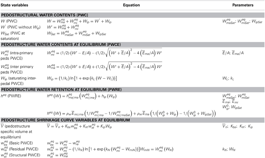
Table 2. The state variables, equations, and parameters of the Pedostructure soil moisture characteristic curves.

Materials and Methods

Soil Samples used for Validation of the Theory

We want to validate the equations established in the theory presented above. For that, we need examples of shrinkage curves and water retention curves that were continuously and simultaneously measured on disturbed or undisturbed soil samples representing the pedostructure of soil medium. Three kinds of shrinkage curves found in the literature have been distinguished according to their shape as shown in Figure 5:

- The shape of the shrinkage curve is clearly sigmoidal (Figure 5A) and there is no saturating interpedal phase due to W_ip at the beginning of the curve near saturation. The three parameters K_bs, K_st, and K_ip of the shrinkage curve Equation (27) are such that: K_bs > 0.3; K_st < 0.1 and K_ip is equal to zero. This case is the most known and studied (Boivin et al., 2004; Braudeau et al., 2004, 2005; Cornelis et al., 2006; Chertkov, 2012).

- The shape is also sigmoidal but the shrinkage curve begins with a clear linear shrinkage phase parallel to the saturation line, due to the departure of the saturating interpedal water W_ip (Figure 5B). This case is typically that of reconstituted pedostructure samples from 2 mm sieved aggregates (Braudeau et al., 1999; Betsogo Atoua, 2010).

- There is no sigmoidal part visible on the shrinkage curve and the different shrinkage phases cannot be distinguished (Figure 5C). In this case, K_st is greater than K_bs and can reach values near 1 while K_ip is taken equal to zero in the shrinkage curve Equation (27). This kind of shrinkage curve is generally observed on silty loam soils of which the aggregated structure is not well developed (Taboada et al., 2008; Salahat et al., 2012).

FIGURE 5

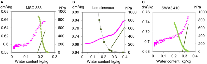
Figure 5. Three types of shrinkage curves (A) sigmoidal; (B) sigmoidal with a saturating interpedal shrinkage phase; and (C) curvilinear structural shrinkage from Betsogo Atoua (2010), Salahat et al. (2012).

Among these three groups, only the first one has examples of simultaneously measured shrinkage and retention curves that had been published (Braudeau and Mohtar, 2004). The device used for these measurements is shown on Figure 4. Two of these examples will be used in the present study. The two other groups will be represented in this study by selected soil samples of which the two characteristic curves were measured simultaneously and with a great accuracy using a new device named TypoSoil™ whose usage methodology is described in the second part of this article. It has been recently designed and built as the successor of the retractometer (Braudeau et al., 1999) to which has been added a device for measuring at the same time the shrinkage and the suction pressure of each of the measured samples (Figure 6). Thus, the soil samples that have been chosen in this study come from two sources differentiated by the device used for the simultaneous measurement of the two curves. A general description of these soil samples is given below and summarized in Table 3.

FIGURE 6

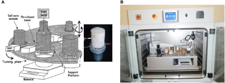
Figure 6. The apparatus TypoSoil™. (A) Schematic drawing for the main components of the apparatus from Braudeau et al. (1999), and (B) Picture of the apparatus while working, one can notice that the apparatus can hold up to eight soil samples where the soil sample's height, diameter, weight, and water succion are taken at 10 min intervals and under the same conditions.

TABLE 3

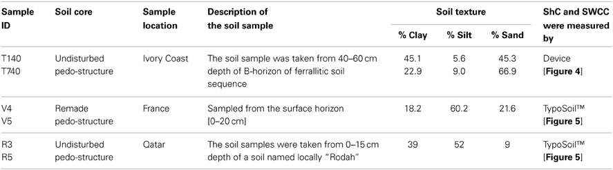
Table 3. General description of the soil samples used in this study.

Source I: Examples of data set measured using the device Figure 4. They are available from the studies of Braudeau and Mohtar (2004) and Braudeau et al. (2005). In these studies the authors made continuous and simultaneous measurement of the soil shrinkage curve and the soil water potential curve on undisturbed cylindrical soil samples (100 cm³). The device (Figure 4) measured at the same time: the weight of the soil sample, its vertical diameter (as shrinkage of the sample was determined from the vertical change in the soil diameter due to the orientation of the soil core in the apparatus), and its water potential. In general, about 400 sets of measurements of the soil sample weight, diameter, and water potential were recorded for each sample.

Source II: The two characteristic curves were measured simultaneously on soil samples selected in this study using the device represented in Figure 6. Two different soil samples have been chosen to represent the two last types of shrinkage curves mentioned above: a soil sample of “Versailles soil” from France, and a soil sample of “Rodah” soil from Qatar.

Two pedostructure samples (prepared in cylinders of 5 cm diameter and height) from a same soil material sieved at 2 mm, known as “Sols du Closeaux à l'INRA de Versailles” (Rousseau, 2003) were reconstituted into the cylinders with a mixture of two different sizes of aggregates: [2–0.2 mm] and [<0.2 mm]. For preparing the soil samples, one kilogram of a disturbed soil was gathered, air dried, and 2 mm-sieved according to the protocol generally used in soil labs to obtain fine ground samples (aggregated soil material <2 mm) ready to analysis. Then, two soil samples labeled V4 and V5 were reconstituted by mixing two different sizes of aggregates according to [54% (coarse) – 42% (fine)] and [72 – 28%], respectively (Betsogo Atoua, 2010).

Two undisturbed soil samples were taken from a “Rodah” soil. Rodah soil is potentially the most suitable soil for cultivation in the State of Qatar (Scheibert et al., 2005). It will be more specifically studied in the second part “application” of this article. The soil samples used in this study have a silty clay loam texture and were given the codes RR3 and RR5 as shown in Table 2.

Fitting Optimization and Estimation of Characteristic Parameters

In order to test and validate the theory and the resulting equations of state of the pedostructure: V (W), h(W), W^eq_ma (W) and W^eq_mi (W), we will use the measured data of the shrinkage and water retention curves of soil samples presented above to optimize the adjustment of the modeled curves which are represented by their characteristic parameters which actually are parameters of their physical equation.

The procedure used for the fittings and for determining the characteristic parameters of the curves was similar to the one used in Braudeau et al. (2004) for the shrinkage curve and in Salahat et al. (2012) for the water potential curve using the Microsoft Excel solver, but with considering the new equations established here for both curves. The sum of square of deviation between the measured and calculated curves was the target to minimalize using the Excel solver within a selected range of water content and according to the selected characteristic parameters put as variable parameters in the solver.

Results and Discussion

Different Kinds of Soil Shrinkage and Water Potential Curves

Figure 7 presents the measured pedostructural shrinkage and water retention curves of each of the soil samples selected for the study. The fitting of these curves using their theoretical equations established above will be presented and discussed in the following section.

FIGURE 7

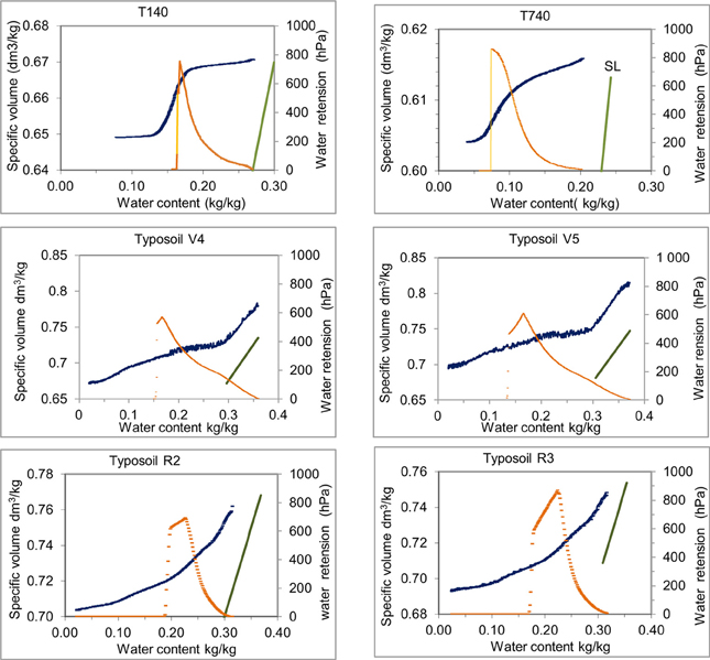
Figure 7. The measured soil shrinkage (blue) and water retention (orange) curves of the soil samples used as examples in this study. The two first samples T140 and T740 were measured in Braudeau and Mohtar (2004) using the device on Figure 4, the others were measured in this study using TypoSoil™.

The following comments can be made:

  (1) The first soil example (the tropical soil, T140, T340) presents the classical sigmoidal shape of shrinkage curve most known in the literature and characterizing well-structured soil mediums (Lauritzen, 1948). The different shrinkage phases: residual, basic, and structural are easily recognizable and the saturating interpedal shrinkage phase due to W_ip is absent or weakly represented. This is an indication of the good cohesion between aggregates of the pedostructure for these soils (Braudeau et al., 2005) and the pedostructural water is exclusively constituted of W_mi and W_ma, such that: W = W^' = W^eq_mi + W^eq_ma in the Equations (26) and (29) of h^eq = h^eq_mi/ma for this kind of soils (oxisols, kaolinitic, structure stable, and well developed).

  (2) The other soil samples do not present this cohesion of structure indicated by the sigmoid shape of the shrinkage curve. However, we must distinguish two cases: (i) the case where a sigmoidal shape of a part of the shrinkage curve is still recognizable such that the points W_N, W_M, and W_L can be roughly positioned on the curve (i.e., Versailles soil “V4 and V5”), and (ii) the case where these points do not appear clearly on the curve as in the Rodah soil “RR3 and RR5.” These two cases can be explained such that:

     • In the first case [Versailles soil “V4 and V5”]: the soil samples present a shrinkage phase corresponding to the departure of W_ip which is clearly identifiable on the shrinkage curve: parallel to the saturated line and in contrast with the structural shrinkage phase due to water change in w_st through evaporation. In this case, W_ip cannot be unheeded such that the total pedostructural water content must be considered as W = W^eq_mi + W^eq_ma + W_ip (Equation 33) where W^eq_ma and W^eq_mi are calculated as a function of W^' = W − W_ip by Equations (26a) and (26b). Also the water retention is in this case: h^eq = h^eq_mi/ma + h_ip calculated using Equations (29) and (32).

     • In the second case: Rodah soil “RR3 and RR5” on Figure 7, the sigmoidal shape does not appear on the shrinkage curve: points N, M, L cannot be positioned. In this case, K_bs is very small compared to K_st which stays however inferior to 1. Accordingly, W_L is fixed equal to W_sat such that W_ip = 0 and W = W^' = W_mi + W_ma in Equations (26) and (29) for the calculus of the different state variables.

Fitting the Measured Curves by the Theoretical Equations

The pedostructure water retention curve h(W) and shrinkage curve V(W) have been established here like state equations corresponding to thermodynamic potential G(T, P, W) and considering T and P constant. These equations are parametric and the adjustment between measured and calculated curves depends thus on the exact value of these parameters, which are also characteristic of the soil structure and its interaction with water. The optimization of the adjustment consists of approaching the closest to the set of the exact values of parameters of the measured curve. If the theoretical equations are correct and the measures accurate, the fit should be almost perfect, validating thus the theory. The procedure of optimization of the adjustment between theoretical and measured curves becomes then a useful mean of determination of the soil characteristic parameters. This procedure of optimization, using Excel and its solver, differs slightly according to the kind of pedostructures quoted above.

Stable (cohesive) and well aggregated pedostructure

This case corresponds to the kaolinitic soils from Ivory Coast [Figures 7A,B]. There is no interpedal shrinkage phase and W_ip = 0 (W_L = W_sat). Results of the fitting of the both characteristic curves of the soil samples T140 and T740 taken as examples are presented on Figure 8. The water retention curve is adjusted first. Then, the shrinkage curve is adjusted using its own parameters.

FIGURE 8

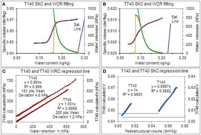
Figure 8. Adjustment of the measured characteristic curves by their theoretical parametric equations for the ferrallitic soil samples T140 and T740. (A,B) Represent for each sample the shrinkage curve (ShC), measured (blue points) and calculated (red line) with its associated water retention curves (WRC), also measured (orange points) and calculated (green line). The quality of the adjustments is illustrated in (C,D) which show the regression line between measured and calculated values for both curves.

Adjustment of the water retention curve. Parameters of the water retention curve h(W) are: W_maSat, W_miSat, E_mi, and E_ma. They are the parameters of Equations (16a) and (16b) for W^eq_ma and W^eq_mi and of Equations (29a) and (29b) for h_ma and h_mi. Figure 8A shows the fit of the water retention curve considered alone, using its parameters as variable parameters. Initialization of the parameters before to run the solver, valuable for all types of soil, is generally done as following:

  • W_miSat is represented on the curve by the point M such that W_M = W_miSat. This point is placed at h = 400 or 500 hPa on the curve as initial value of the optimization.

  • W_maSat is replaced by W_Sat = W_maSat + W_miSat as variable parameter; the initial value or fixed value of W_Sat is chosen at the beginning or at h = 0 kPa of the water retention curve.

  • E_mi is the quantity of surface charges of the clay-particles inside the primary peds and will be initialized at 40 J/kg.

  • E_ma, the charges at the external surface of primary peds, is replaced by E/E_ma as variable parameter which is generally initialized at 100.

The adjustment of the water retention curve is always excellent, as shown as example in Figures 8A,B for the sample T140. The deviation between the measured and calculated values does not exceed 10 hPa all along the range of validity of the tensiometer curve (here: 8–680 hPa). The values of parameters are given in Table 4.

TABLE 4

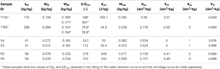
Table 4. Pedostructure thermodynamic equilibrium parameters calculated from the shrinkage curve and the water tension curve of the soil (pedostructure) samples.

Adjustment of the shrinkage curve. For fitting the shrinkage curve, K_bs is fixed to its value read on the curve (slope at point B) and the initialization of parameters concerns k_N, W_N, W_M, E/E_ma, that are such that: k_N = 100, W_N and W_M take the values read on the shrinkage curve according to the corresponding shrinkage phases (see Figure 3) and E/E_ma = 1.0. The adjustment of the shrinkage curve considered alone is always excellent as shown on Figure 8D; however, as we can see on Table 4, the parameters W_M and E/E_ma do not correspond to those found in the water retention adjustment.

We will see further that this discrepancy between the values of W_M and E/E_ma for the two curves does not appear with the data measured using TypoSoil™. It might be caused by the approximate calculus of the volume which used only the vertical measurement of the diameter of the sample (see Figure 4) as variable in the old method, compared to the tridimensional measurement of the soil sample in the new method (Figure 6).

Weakly consistent and little aggregated pedostructure

The sigmoidal shape is recognizable along with a saturated interpedal shrinkage phase parallel to the saturation line (Figure 5). This is the case of [Versailles soil “V4 and V5”: Figures 6B,C]. For these soil samples, the two types of water: W^eq_ma (≡ w_st) and W_ip (≡ w_ip), are well distinguished on the shrinkage curve by the point L (Figure 3) such that, at saturation, W_sat = W^eq_miSat + W^eq_maSat + W_ipSat with W_ipSat = W_sat − W_L. The pedostructure water retention at equilibrium is h^eq = h^eq_mi/ma + h_ip and, in this case, we have to add three new parameters to the four parameters in the previous case: W_L and k_L, parameters of the w_ip Equation (23), and W⁰_ip which is the constant of adjustment in Equation (32). Initialization of the added parameters is as following: W_L is read approximately on the shrinkage curve, k_L is put at 80 kg/kg and W⁰_ip equal to W_maSat/2.

The adjustment of both curves is made in two times. The shrinkage curve is fitted in first using k_N, W_N, W_M, E/E_ma, k_L, and W_Las variable parameters. As for the previous case, K_bs is fixed to its value calculated from the curve. The adjustment of the shrinkage curve is made in once without any difficulty. Then, the two curves are fitted jointly minimizing the product of the sum of squares of deviation of the two curves and using the following variable parameters: W_M, E/E_ma, E_mi, W⁰_ip, k_L, and W_L; W_Sat being fixed at its value at h = 0.

Adjustments are excellent as we can see on Figure 9 for the Versailles soil samples. Figures 9A,B show the adjustment of the two curves made conjointly for the two samples V4 and V5. Results are given in Table 4. Their characteristic parameters are very similar, indicating the good replicability of the samples manufacturing from the 2 mm sieved soil material. The quality of the adjustments can be seen on Figures 9C,D that show the regression lines between measured and calculated data for the two curves and for each sample. The fits of the water retention curves are particularly impressive: they are almost perfect within the range of validity of their measure that represents about 280 points: the maximum of absolute deviation being 5 hPa and the average less than 2.2 hPa.

FIGURE 9

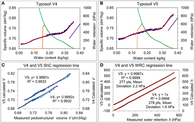
Figure 9. Adjustment of the measured characteristic curves by their theoretical parametric equations for the Versailles soil type, V4 and V5. (A,B) represent for each sample the shrinkage curve (ShC), measured (blue points) and calculated (red line) with its associated water retention curves (WRC), also measured (orange points) and calculated (green line). The quality of the adjustments is illustrated in (C,D) which show the regression line between measured and calculated values for both curves.

Consistent but non-aggregated pedostructure

No sigmoidal part of the shrinkage curve, it corresponds to the residual, basic and structural shrinkage phases, with K_st > K_bs. This case is that of the Rodah soil samples. There are no mark on curves that might indicate the position of points L and M. The samples will be treated in the fitting of curves like in the first case where the pedostructural water content is composed of only W_mi and W_ma in equilibrium of potential in the macro and micropore spaces: W = W_mi + W_ma. The difference with the first case, where K_st was considered near or equal to zero, is that the removal of the structural macropore water w_st provokes a shrinkage of the medium with a strong slope of value intermediary between K_bs and 1.

The fit of the water retention curve can be made alone and is made in first, determining the four characteristic parameters: W_M(= W_miSat), E/E_ma, E_mi and W_sat. The same excellent fits are obtained as above, providing the accurate values of these parameters, which can be seen on the Figure 10. Then, the adjustment of the shrinkage curve is done using the parameters already fund and the following variable parameters: k_N, W_N, K_bs, and K_st of the shrinkage curve only. Initialization of variables is like for the cases above.

FIGURE 10

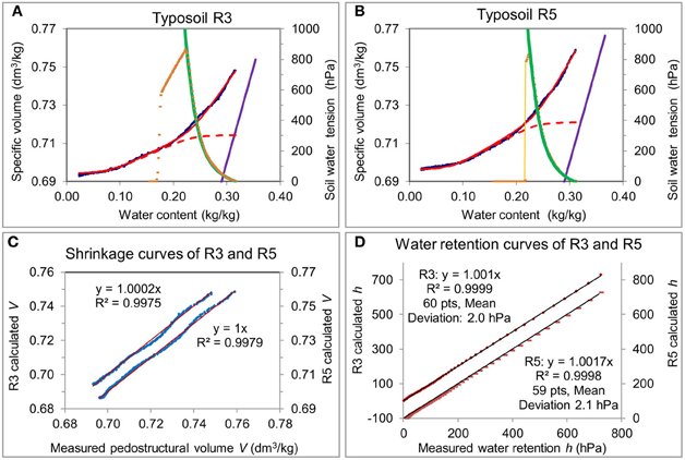
Figure 10. Adjustment of the measured characteristic curves by their theoretical parametric equations for two non-disturbed pedostructure samples of the Rodah soil, R3 and R5. (A,B) represent for each sample the shrinkage curve (ShC), measured (blue points) and calculated (red line) with its associated water retention curves (WRC), also measured (orange points) and calculated (green line). The quality of the adjustments is illustrated in (C,D) which show the regression line between measured and calculated values for both curves.

Figure 10 shows the good adjustments of the two curves of soils represented by Rodah soils; in particular the measured and modeled water retention curves are almost superimposed on the Figures 10A,B for the two samples. The excellent quality of these adjustments can be appreciated on Figures 10C,D representing linear regressions between measured and calculated data of the two curves. Moreover, the two Rodah samples that were sampled in the same location have curves of similar shapes; this is reflected by near values of their parameters in Table 4. It is an illustration, like in the previous case, of the good reproducibility of the measurement method and of the procedure of adjustment of the curves based on the use of their theoretical parametric equations.

Discussion

Comparison with the previous equations of the soil water potential curves

For each sample analyzed, the coefficient of regression between measured and calculated water retention curves was very closed to 1. This implies that the parameter σ in Equation (2) of h_ma (W_ma) proposed before by Braudeau et al. (2004) is not needed. In fact, the role of σ introduced by these authors was to allow the fit of h_ma calculated by Equation (2) on the reading of the tensiometer including the zone out of its validity where bubbles of water vapor have taken place in the tensiometer tube. Their hypothesis was that the tensiometer reading corresponded exactly to the water potential of the macropore interpedal water (W_ma), which is also our hypothesis, but they considered the relation h = h_ma without the condition of h = h_ma = h_mi. Thus, the σ term was introduced in the equation of h_ma and was ambiguously defined as transitional micro-poral water content at the interface with the macropore (interpedal) space; it was considered as one of the parameters of the water potential curve in few studies based on the pedostructure concept (Salahat et al., 2012; Singh et al., 2012). However, if we apply the constraint of (h = h_mi = h_ma) in the adjustment of the old equations of W_ma, W_mi, h_ma, and h_mi Equations (1a, 1b) and (2a, 2b) on a measured water retention curve h(W), we obtain almost the same results as if the new equations were used. Doing this, the obtained value for σ is near to zero and the calculated curves of w_st (old equation) and W_ma (new equation) are superimposed as shown on Figure 11. The surprising result is this quasi-equivalence of shape between Equations (1) and (19) for W_ma and (2) and (20) for W_mi (Figure 11). The essential difference stays in the fact that Equations (19) and (20) contain by themselves the constraint (h = h_mi = h_ma) so we can use only one of the two equations to express the water retention curve, unlike the former Equations (1) and (2) that must be used together in the fitting of the measured water potential curve. This constraint of equality of potentials was already applied in Kamel^® and KamelSoil computer models (Braudeau et al., 2009) and in the other works mentioned above referring to the pedostructure concept (Mallory et al., 2011; Salahat et al., 2012; Singh et al., 2012).

FIGURE 11

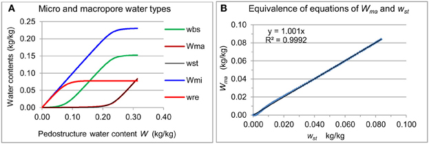
Figure 11. Hydrostructural characterization and modeling of the Rodah soil sample R3. (A) contents according to the total pedostructure water content W, of the different micro and macro-pore water types; and (B) comparison of the macropore water content W_ma calculated by the new and the old physical equation used for W_ma and w_st respectively.

Validation of the Theory

The great assumptions that were made in the thermodynamic theory of the soil water (Sposito, 1981) for deducing the two soil moisture characteristic curves, h(W) and V(W) (at T and P constant) that have been validated here, were:

(i) The soil medium organization is well described by the pedostructure concept which defines its first levels of organization and the descriptive variables of its hydro-functional components, like W_mi, W_ma, W_ip.

(ii) W_mi and W_ma are two distinct physical components of the soil water phase whose the thermodynamic potentials G_mi(T, P, W_mi) and G_ma(T, P, W_ma) are equal to, respectively, E_mi and E_ma which are the potential energy of the surface charges of the clay particles, respectively inside and at the surface of primary peds. Therefore, G_mi and G_ma stay constant during a change in water content because the pedostructure organization stays stable (and so the clay surface charges distribution) in the wetting-drying cycles.

The excellent adjustments obtained of measured and theoretical curves confirm not only the validity of equations and parameters of these curves but also the systemic and thermodynamic approach that were used for finding their formulation.

Hydro-Functional Typology of Soils

We could see that two important characteristics of the clay mineral and of their arrangement in aggregates (E = E_mi + E_ma and E/E_ma) are easily extracted from measured water potential curves, as well as the maximum of water content possible into the both intra and inter primary peds pore space of the pedostructure: W_miSat and W_maSat. In fact the four parameters [W_miSat, W_maSat, E_mi, and E_ma] characterize the hydrostructural equilibrium of this arrangement in aggregates, the pedostructure.

An important implication of this hydro-thermodynamic equilibrium modeling of the soil medium is the possibility of establishing a functional typology of soils based on the hydrostructural characterization of its pedostructures. The typology of soils is to restart since pedostructure is now precisely defined as a thermodynamic system which is therefore completely characterized by the knowledge of its equations of equilibrium state [V(W) and h(W)] represented by their hydrostructural parameters. This thermodynamic typology of pedostructures would allow the linkage between different disciplines of the soil sciences such as soil mapping with remote sensing, biophysical modeling, and especially experiments in the laboratory of such characterized soil sample for analysis of biological processes in the soil medium.

Conclusions

These initial results demonstrate conclusively that there is no physical characterization without the acknowledgement of the hydrostructural and thermodynamic equilibrium of the soil medium organized in primary aggregates made of solid particles, such as clay particles, immersed in water, arranged in layers surrounding these particles, and itself surrounded by the air. We could not find the thermodynamic equation h(W) without resting the fundamentals of the soil water thermodynamics on the soil medium organization and the acknowledge of the two components W_mi and W_ma of the pedostructural water phase.

In this article, the distinction of the soil water content into two nested fractions, located inside and outside of the clayey plasma of the pedostructure, as previously evidenced by the shrinkage curve, has been physically and mathematically justified using a systemic and thermodynamic approach of the primary soil medium organization: the pedostructure. All the equations presented are based on the concept of pedostructure as a SREV of the soil medium in a soil horizon. The excellent adjustments obtained of the thermodynamic equations on the measured curves confirm the validity of these equations and their parameters, and also the systemic and thermodynamic approach that were used for finding their formulation. Applying the SREV concept to the current thermodynamic theory of the soil water led us to reformulate the two principal characteristic curves of the soil moisture in the frame of the thermodynamics of organization of the soil medium. These findings pave the way for a thermodynamic formulation of all exchanges (heat, space, solutions, gas) between biological organisms living in the soil and the soil medium itself which offers the physical conditions for their activities and development.

Conflict of Interest Statement

(1) The apparatus used in the work presented in the article to validate the theory was recently (2013) patented conjointly by IRD and Valorhiz (of which the CEO is Hassan Boukcim); Erik Braudeau is one of the two inventors. (2) The same for the method of obtaining the pedostructural parameters: patented by IRD and Valorhiz; Erik Braudeau inventor.

References

Ahuja, L. R., Ma, L., and Timlin, D. J. (2006). Trans-disciplinary soil physics research critical to synthesis and modeling of agricultural systems. Soil Sci. Soc. Am. J. 70, 311–326. doi: 10.2136/sssaj2005.0207

CrossRef Full Text

Berezin, P. N., Voronin, A. D., and Shein, Y. V. (1983). An energetic approach to the quantitative evaluation of soil structure. Pochvovedeniye 10, 63–69.

Betsogo Atoua, A. (2010). Caractérisation hydrostructurale d'un sol limoneux appliquée à l'étude de la croissance d'un champignon filamenteux dans le sol. Mémoire de Master, Université Paris-Est Créteil/IRD, 66.

Boivin, P. (2007). Anisotropy, cracking, and shrinkage of vertisol samples. Experimental study and shrinkage modeling. Geoderma 138, 25–38. doi: 10.1016/j.geoderma.2006.10.009

CrossRef Full Text

Boivin, P., Garnier, P., and Tessier, D. (2004). Relationship between clay content, clay type, and shrinkage properties of soil samples. Soil Sci. Soc. Am. J. 68, 1145–1153. doi: 10.2136/sssaj2004.1145

CrossRef Full Text

Braudeau, E. (1988). Équation généralisée des courbes de retrait d'échantillons de sols structurés. C. R. Acad. Sci. Paris 307, 1731–1734.

Braudeau, E., and Bruand, A. (1993). Détermination de la courbe de retrait de la phase argileuse à partir de la courbe de retrait établie sur échantillon de sol non remanié. C.R. Acad. Sci. Paris 316, 685–692.

Braudeau, E., Costantini, J. M., Bellier, G., and Colleuille, H. (1999). New device and method for soil SC measurement and characterization. Soil Sci. Soc. Am. J. 63, 525–535. doi: 10.2136/sssaj1999.03615995006300030015x

CrossRef Full Text

Braudeau, E., Frangi, J. P., and Mothar, R. H. (2004). Characterizing non-rigid dual porosity structured soil medium using its shrinkage curve. Soil Sci. Soc. Am. J. 68, 359–370. doi: 10.2136/sssaj2004.3590

CrossRef Full Text

Braudeau, E., and Mohtar, R. H. (2004). Water potential in non-rigid unsaturated soil-water medium. Water Resour. Res. 40, W05108, 14. doi: 10.1029/2004WR003119

CrossRef Full Text

Braudeau, E., and Mohtar, R. H. (2009). Modeling the soil system: bridging the gap between pedology and soil-water physics. Global Planet. Change J. 67, 51–61. doi: 10.1016/j.gloplacha.2008.12.002

CrossRef Full Text

Braudeau, E., Mohtar, R. H., El Ghezal, N., Crayol, M., Salahat, M., and Martin, P. (2009). A multi-scale “soil water structure” model based on the pedostructure concept. Hydrol. Earth Syst. Sci. Discuss. 6, 1111–1163. doi: 10.5194/hessd-6-1111-2009

CrossRef Full Text

Braudeau, E., Sene, M., and Mohtar, R. H. (2005). Hydrostructural characteristics of two African tropical soils. Eur. J. of Soil Sci. 56, 375–388. doi: 10.1111/j.1365-2389.2004.00679.x

Pubmed Abstract | Pubmed Full Text | CrossRef Full Text

Chertkov, V. Y. (2012). Physical modeling of the soil swelling curve vs. the shrinkage curve. Adv. Water Res. 44, 66–84. doi: 10.1016/j.advwatres.2012.05.003

CrossRef Full Text

Cornelis, W. M., Corluy, J., Medina, H., Díaz, J., Hartmann, R., Van Meirvenne, M., et al. (2006). Measuring and modelling the soil shrinkage characteristic curve. Geoderma 137, 179–191. doi: 10.1016/j.geoderma.2006.08.022

CrossRef Full Text

El Kadi, A. I. (1985). On estimating the hydraulic properties of soil, Part 1. Comparison between forms to estimate the soil- water characteristic function. Adv. Water Resources 8, 136–147. doi: 10.1016/0309-1708(85)90054-5

CrossRef Full Text

Lauritzen, C. W. (1948). Apparent specific volume and shrinkage char- acteristics of soil materials. Soil Sci. 65, 155–179. doi: 10.1097/00010694-194802000-00003

CrossRef Full Text

Leij, F., Russell, W., and Lesch, S. M. (1997). Closed-form expressions for water retention and conductivity data. Ground Water 35, 848–858. doi: 10.1111/j.1745-6584.1997.tb00153.x

CrossRef Full Text

Low, P. F. (1987). Structural component of the swelling pressure of clays. Langmir 3, 18–25. doi: 10.1021/la00073a004

CrossRef Full Text

Mallory, J., Mohtar, R., Heathman, G., Schulze, D., and Braudeau, E. (2011). Evaluating the effect of tillage on soil structural properties using the pedostructure concept. Geoderma 163, 141–149. doi: 10.1016/j.geoderma.2011.01.018

CrossRef Full Text

Rieu, M., and Sposito, G. (1991). Relation pression capillaire-teneur en eau dans les milieux poreux fragmente's et identification du caracte 're fractal de la structure des sols. C. R. Acad. Sci. 312, 1483–1489.

Rousseau, M. (2003). Transport préférentiel de particules dans un sol non saturé:de l'expérimentation en colonne lysimetrique à l'élaboration d'un modèle à base physique. Grenoble: Thèse Institut National Polytechnique de Grenoble.

Salahat, M., Mohtar, R., Braudeau, E., Schulze, D., and Assi, A. (2012). Toward delineating hydro-functional soil mapping units using the pedostructure concept: a case study. Comput. Electron. Agr. 86, 15–25. doi: 10.1016/j.compag.2012.04.011

CrossRef Full Text

Scheibert, C., Stietiya, M., Sommer, J., Schramm, H., and Memah, M. (2005). “The atlas of soils for the State of Qatar,” in Soil Classification and Land Use Specification Project for the State of Qatar, eds Ministry of Municipal Affairs and Agriculture, General Directorate of Agricultural Research and Development, Department of Agricultural and Water Research (Doha: Ministry of Municipal Affairs and Agriculture), 19–36.

Singh, J., Mohtar, R., Braudeau, E., Heathmen, G., Jesiek, J., and Singh, D. (2012). Field evaluation of the pedostructure-based model (Kamel). Comput. Electron. Agr. 86, 4–14. doi: 10.1016/j.compag.2012.03.001

CrossRef Full Text

Sposito, G. (1981). The Thermodynamics of Soil Solutions. New York, NY: Oxford University Press, 187–208.

Sposito, G., and Giraldez, J. V. (1976). Thermodynamic stability and the law of corresponding states in swelling soils. Soil Sci. Soc. Am. J. 40, 352–358. doi: 10.2136/sssaj1976.03615995004000030016x

CrossRef Full Text

Taboada, M. A., Barbosa, O. A., and Cosentino, D. J. (2008). Null creation of air-filled structural pores by soil cracking and shrinkage in silty loamy soils. Soil Sci. 173, 130–142. doi: 10.1097/SS.0b013e31815d8e9d

CrossRef Full Text

Voronin, A. D. (1980). The structure-energy conception of the hydrophy- sical properties of soils and its practical applications. Pochvovedeniye 12, 35–46