Brackish groundwater membrane system design for sustainable irrigation: optimal configuration selection using analytic hierarchy process and multi-dimension scaling

Introduction

Reuse of brackish water, mainly for agricultural irrigation, simultaneously solves water shortage problem and allows for overcoming environmental pollution problems (Qadir et al., 2007; Ghermandi and Mesalem, 2009). It is recognized that water for irrigation should be without particles with average size larger than 50–100 micron and, have a low salt content to avoid certain ion toxicities and increase of soil salinity (Ben-Gal et al., 2008; Edelstein et al., 2009). Salt concentration is generally tested by electrical conductivity (EC) or total dissolved solids (TDS) levels (Bui, 2013). In addition, the sodium to water hardness (calcium and magnesium) ratio should be managed to keep sodium absorption ratio (SAR) at values lower than 3–4, if possible. Together with that, precipitation potential of the water should be to some extent negative in order to avoid the precipitation of calcium and magnesium on the productive system. Also, iron and manganese ions need to be managed to prevent staining harms.

Other parameters, such as boron, fluoride, and heavy metals should also be low to ease the possibility of ion toxicity. Besides, irrigation water needs to be without any disease-causing microorganisms, viruses, bacteria, fungi, nematodes, cysts, etc. (Yermiyahu et al., 2007; Bustan et al., 2013).

Hence, irrigation water has to be treated properly to get rid of all the undesirable physical, chemical, and biological contaminants that are able to: (i) reduce the choice of crops (Levy and Tai, 2013); (ii) cut down crop yield (Rasouli et al., 2013); (iii) damage crop quality (Bernstein et al., 2011); (iv) injure soil appropriateness (Liu et al., 2013); and (v) harm the irrigation tools (Connor et al., 2012).

Water treatment regarding irrigation purposes is quite new to the agricultural business. The advanced technology is based on membrane technology (Oron et al., 2008; Bick et al., 2012). Mainly, NanoFiltration (NF) and Reverse-Osmosis (RO) can usually be implemented for removal of organic matter, particles, turbidity, pathogenic micro-organisms, and selective ions without the use of disinfectants (Mrayed et al., 2011; Riera et al., 2013).

Membrane system presents several advantages: modularity, automation, low maintenance costs, and low chemicals consumption (Miller, 2006; Birnhack et al., 2010). However, there are several drawbacks: high energy consumption, permeate quality (lack of vital ions for plant growth, e.g., magnesium), high costs relative to other sources of water and in particular chemical and biological fouling of the membranes (Oren et al., 2012).

For a known feed water source, the selection between membrane and any other alternative for water treatment is usually made on technical, economical, and/or political criteria. Yet, environmental concern have demonstrated its importance to integrate sustainability factors into the judgment process by comparing the “green” impacts of the different alternatives (Vince et al., 2008; Lew et al., 2009).

Downstream supervision on desalination plants, such as brine dilution, treatment, and/or removal may diminish the ecological impacts. However, reducing the upstream sources through means of optimization may be more successfully in minimizing the environmental impacts. The actual performances of the membrane course of action outcome from model choices, which usually are designed to minimize the total water cost, taking in account technical constraints and project necessities but, with no consideration for the environmental impact (Bartels et al., 2008; Garcia et al., 2013; Wei et al., 2013). The environmental performances of the membrane system could be enhanced by revaluating these previously defined outline selections (Gur-Reznik et al., 2011; Chakrabortty et al., 2013; Zheng et al., 2013; Zhou et al., 2013). It is thus anticipated the introduction of the environmental criteria directly in the near the beginning design phases, in order to classify environmental responsible process configurations (Vince et al., 2008).

Concerning agricultural applications, NF membranes showed up to be a new opportunity for salty water desalination (Hilal et al., 2005): (i) high rejection rate for divalent ions, capability of knocking down TDS significantly and may constitute a potentially cost-effective alternative for irrigation with brackish water; (ii) higher tolerance (in general) for fouling conditions, as compared to RO (Gutman et al., 2012; Sotto et al., 2013); (iii) removal of specific pollutants, so that the concentrate stream can be used without increased membrane fouling; and (iv) operation at lower applied pressures, as compared to RO, saving energy and operating costs (Nederlof et al., 2005; Al-Amoudi and Lovitt, 2007; Zhao et al., 2012).

NF-RO configuration can be a promising solution, since (i) the NF stage can separate the agriculturally advantageous ions, such as magnesium from the non-desirable ions, such as sodium, which are finally removed from the water by the following RO stage; and (ii) the advantageous ions (in the NF brine flow) can be blended with the free sodium water produced in the RO stage (RO permeate stream) to create a nutrient-enriched, low-salt water (Mrayed et al., 2011).

The Arava Valley in Israel was used for this study, and the modeling and design of a desalination plant featuring both NF and RO membranes is discussed. The objectives of this study are: (i) to examine the designs of NF and RO membranes using typical brackish water from Hatzeva-Idan aquifer in the Arava Valley (Israel), which is characterized to some extent by saline water with a typical TDS concentration of 1200 ppm; (ii) to simulate RO and NF technologies for desalination of brackish water (using IMSDesign software, Verhuelsdonk et al., 2010; Karabelas et al., 2012); (iii) to compare the design configuration using Analytic Hierarchy Process (AHP) model (Caputo et al., 2013); and (iv) to rank the various alternatives using multi-dimension scaling (MDS) technique (Lespinats et al., 2009) in order to find the optimal design configuration for technology selection.

Materials and Method

Management Modeling and the Analytical Hierarchical Process (AHP)

The amount of data and information collected and retained by organizations and businesses is persistently growing, due to advances in data gathering, computerization of transactions, and breakthroughs in storage tools. In order to take out practical information from such large datasets, it is crucial to be able to spot patterns, trends and interactions in the data and visualize their global configuration to ease decision making. Decision making techniques used for the ranking of various options on the basis of more than one attribute are strictly dependent on the attributes setting and thus can be completely different for different settings (Saaty, 1980).

The analytical hierarchical process (AHP) is a strong and flexible decision-supporting process that helps in setting priorities and making the best decision when mutually qualitative and quantitative aspects are measured (Tzfati et al., 2011; Zhang et al., 2013). The AHP is designed for individual evaluation of a set of options based on multiple attributes, and is approved in a hierarchical building (Kayastha et al., 2013). The estimate of the options is founded on a pair-wise judgment (Bozoki et al., 2011). The pair-wise comparisons are translated from linguistic/verbal expressions in numerical values (integers 1–9) using the original Saaty's Scale (Saaty, 2003) for the comparative judgments (Table 1).

TABLE 1

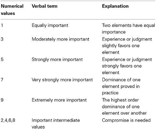
Table 1. Fundamental Saaty's Scale for pair-wise comparison (Saaty, 1980).

Multi Dimension Scaling (MDS) and CoPlot

Many research questions dealing with information require the analysis of complex multivariate data (Gomez-Silvan et al., 2013). Briefly, most multivariate approaches can be roughly classified as dependence methods (e.g., multiple regression, discriminant analysis, multivariate analysis of variance), that are usually used to assess the relationship between dependent and independent variables; or as interdependence methods (e.g., principal component analysis, factor analysis, cluster analysis), that are typically used to estimate the mutual association among all variables with no difference made among the variable types (Schilli et al., 2010). Multi dimensional scaling (MDS) is an interdependence methods that facilitates the examination of multivariate data by reducing multidimensional data into a two-dimensional structure that attempts to expose the “out of sight structure” in a data set by creating a pictorial or mapping image of the data. The MDS map graphically represents the proximities (or similarities) between objects (i.e., observations or events). Similarities between the observations in the data set are transformed into distances on a map such that observations with great similarity are closer together than less similar observations.

In this way, a single picture illustrates the relationships among all the observations. MDS, initially developed in the 1960s, has been used to evaluate the relationships among observations, to identify clusters of similar observations and to locate outliers (Bick et al., 2011). However, MDS maps have two key limitations: (i) MDS does not simultaneously map the variables and the observations; and (ii) the MDS map has no orientation, thereby limiting the map's interpretability.

CoPlot, a variant of multi-dimensional scaling, addresses both these limitations and locates each decision-making unit in a two-dimensional space in which the location of each observation is strong-minded by every variables simultaneously (hence, its name) (Lipshitz and Raveh, 1994). The graphical put on view technique exhibits observations as points and variables as arrows, relative to the same center-of-gravity. CoPlot is rooted in the integration of mapping concepts, using a variant of regression analysis that superimposes two graphs sequentially. Additionally, CoPlot maps the observations and variables in a manner that preserves their relationships, allowing richer interpretations of the data. Importantly, CoPlot allows analysis of a dataset where the number of variables is greater than the number of observations. Also, CoPlot map can be used to detect outliers and errors in the data, assessment of the relationships within the data and for selection of key variables for subsequent analysis (Adler and Raveh, 2008).

Coplot's output is a visual display of its findings [Given an input matrix Yn × v of v variable values for each of n observations (see for example Table 2)] and it is based on two graphs that are superimposed on each other (Bravata et al., 2008). The first graph maps the n observations into a two-dimensional space: those observations that are perceived to be very similar to each other are placed near each other on the map, and those observations that are perceived to be very different from each other are placed far away from each other on the map. The second graph (Figure 1) consists of v arrows, representing the variables and it shows the direction of the gradient for each arrow.

TABLE 2

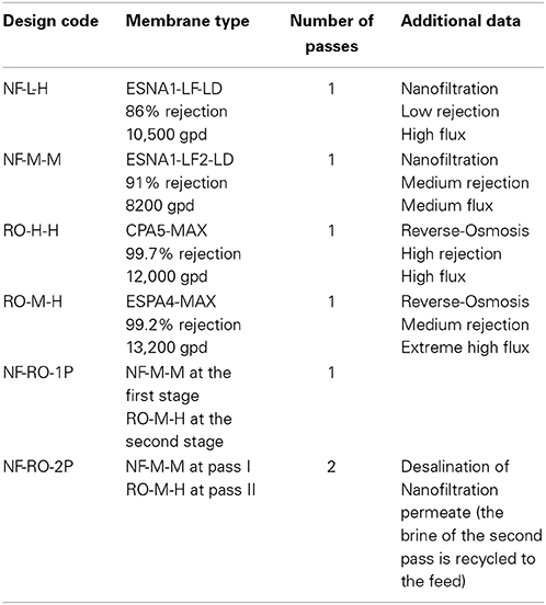
Table 2. Production technologies for irrigation.

FIGURE 1

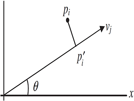
Figure 1. CoPlot: Adding the variable vectors. The point p_i corresponds to the coordinates for observation i = 1, …, n. The vector v_j is for the variable j = 1, … m. The x-axis is rotated through an angle θ to give a point p′_i, which is the projection of p_i onto the vector v_j. The correlation between the n new projected scores and the original n values for variable j are computed, and the choice for θ is the one that maximizes this correlation.

The CoPlot analysis consists of four stages, two preliminary adaptations of the data matrix and two subsequent stages that compute two maps sequentially that are then superimposed to produce a single map. The goal of the first stage is to normalize the variables, which is needed in order to allow the variables to relate to each other, although each variable has a different unit and scale. This is done in the usual way, the difference between the elements of the matrix Y_ij (which are scores) and the deviations from column meansY_j is divided by their standard deviations (D_j), given the normalized Z_ij, according to Equation (1).

$\begin{array}{cc}{Z}_{ij}=\left(Y_{ij-}{\overline{Y}}_j\right)/D_j& (1)\end{array}$

In the second stage, a measure of dissimilarity (S_ik ≥ 0) between each pair of observations (rows of Zn × v) is chosen and a symmetric n × n matrix is produced from all the different pairs of observations. To measure S_ik, the sum of absolute deviations (generally defined as city-block distance) as a measure of dissimilarity is used (Equation 2).

$\begin{array}{cc}{S}_{ik}={\displaystyle \sum _{j=1}^v\left|Z_{ij-}{Z}_{kj}\right|}& (2)\end{array}$

In the third stage the matrix S_ik is mapped by a MDS method. The algorithm maps the matrix S_ik into an Euclidean space, of two dimensions in our case, such that “similar” observations (with a small dissimilarity between them) are close to each other on the map, while “different” ones are also distant on the map. Formally, the requirement is as follows: consider two observations, i and k, which are mapped at a d_ik distance from each other. This distance has to reflect the dissimilarity S_ik (which is actually a relative measurement), taking in consideration that the important constraints are S_ik < S_lm if d_ik < d_lm.

CoPlot procedure uses the Guttman's smallest space analysis (SSA) with the “coefficient of alienation” (Θ) as a measure of “goodness of fit” (Guttman, 1968; Raveh, 2000). The intuition for Θ comes directly from the above MDS requirement of dissimilarity measures and the map distances: A success of satisfying it implies that the product of the differences between the dissimilarity measures and the map distances are positive. In a normalized form a new variable is defined, μ_ca (Equation 3).

$\begin{array}{cc}{\mu }_{ca}=\frac{{\displaystyle {\sum }_{i,k,l,m}\left(S_{ik}-S_{lm}\right)}\left(d_{ik}-d_{lm}\right)}{{\displaystyle {\sum }_{i,k,l,m}\left|S_{ik}-S_{lm}\right|}\left|d_{ik}-d_{lm}\right|}& (3)\end{array}$

μ_ca can attain a maximal value of 1 (Raveh, 2000) and is used to define Θ according to Equation (4).

$\begin{array}{cc}\Theta =\sqrt{1-{\mu }_{ca}^2}& (4)\end{array}$

The details of the SSA algorithm are beyond the scope of this paper and were presented in the literature (Guttman, 1968). The SSA algorithm is an extensively used method in social sciences and several examples along with intuitive descriptions can be found (Raveh, 2000). The outcome of this stage is a two-dimensional map of n observations and the CoPlot user can color code observations with any definite variable that has up to 16 different values.

The map generated so far is a classical MDS map, however without orientation or meaningful axes. In the fourth stage of the CoPlot method, v arrows are drawn on the Euclidean space previously obtained. Each variable j is represented by an arrow j, emerging from the center of gravity of the n points. The graphical display technique plots observations as points and variables as arrows, relative to the same arbitrary center-of-gravity. Observations are mapped such that similar entities are closely located on the plot, signifying that they belong to a group possessing comparable characteristics and behavior. The location of the center of gravity is in the middle of the plot in order to introduce all the observations and it does not affect the arrows direction. The direction of each arrow is selected so that the correlation between the actual values of the variable j and their projections on the arrow is maximal (the arrows' length is undefined). Therefore, observations with a high j value will be located in the part of the space which the arrow points to, while observations with a low j value will be located at the other side of the map. The magnitude of the j maximal correlations measures the “goodness of fit” of the R_j regressions. Higher is the correlation better is the arrow representation of the variables and, those having low correlations should be eliminated.

Moreover, arrows linked with highly correlated variables will point in about the same direction and vice versa. As a result, the cosines of angles between these arrows are approximately proportional to the correlations between their associated variables (Raveh, 2000).

The “goodness of fit” measured for each correlation (R_j) is obtained as follows: For each possible variable vector, CoPlot projects the points onto the vector, thereby yielding n projected values. These projected values can now be compared with the observed values. The axis that is chosen is the one that maximizes the correlation between the projected values and the observed values. Figure 1 depicts how this is performed. The point p_i corresponds to the coordinates for observation i = 1, …, n. The vector v_j is for the variable j = 1, …, m. The x-axis is rotated through an angle θ to give a point p′_i, which is the projection of p_i onto the vector v_j. The correlation between the n new projected scores and the original n values for variable j are computed and, the choice for “goodness of fit” is the one that maximizes this correlation. This maximization can be achieved numerically by calculating all 360° possibilities for θ, which is performed separately for each variable vector.

These variable vectors have four useful properties; first, vectors for highly correlated variables point in the same direction, vectors for highly negatively correlated variables are oriented along the same axis but in opposing directions and, vectors for variables that are not correlated are orthogonal to each other. Second, each vector emanates from the center of gravity, which serves as the origin. An observation located at or near the origin is an average observation (it has an average value in all variables). Third, the length of each vector is proportional to the correlation (namely R_j) between the original data for that variable and the projections of the observations onto the vector. Finally, the cosines of angles between the arrows are approximately proportional to the correlations between their associated Variables. Therefore, the correlational structure among the variables can be studied in a single graphical output (Raveh, 2000).

In practical terms, the user imports data, selects variables and observations for inclusion in the analysis, creates the CoPlot map, evaluates Θ parameters, selects the map to view (observations only, variables only, or both observations and variables) and, then selects variables for color coding the observations for greater interpretation. Qualitative variables can be selected for color coding and may either be included in the computation of the map or can be excluded from the computation of the map but still used for color coding. For example, if a variable was found to have low R_j, it might be excluded from the computation of the map but could still be used to color code variables to facilitate the interpretation of the data.

CoPlot produces two “goodness of fit” measurements, one that describes how well the CoPlot map represents the observations and another that describes how well the CoPlot map represents the variables. The first measure is a “coefficient of alienation” (Θ), which indicates the relative loss of information that arises when the multidimensional data are transformed into two dimensions. The lower the Θ value, the smaller the information loss in the process of reducing the original data set to a two-dimensional map. In other words, the lower the Θ, the more precise the representation of the MDS model to the proximities. A general rule-of-thumb states that the map is statistically significant if Θ ≤ 0.15 (Guttman, 1968).

In general, as the number of variables increases, Θ also increases. In such case, Θ measures the discrepancy between every pair of points and the original matrix of “similarities” that comprises distances between points, so that this index provides a comparison between two matrices, the matrix similarities (which are inputs) and the matrix of the distances on the map (which are outputs) obtained by the algorithm. When these two matrices (inputs and outputs) are identical, Θ is zero (precise).

The second “goodness of fit” measure is obtained at the stage of calculating the correlation between the original data, for each variable and, the projection of each observation onto that vector in the CoPlot map. In general, the methodology maximizes the correlations (actually the normalized cross-products) of the vector of inputs (the actual distances from each point to every other point) and the outputs (the coordinates of the vectors that go into the map); in other words, the R_j measurements are the correlational measure that relates the input with the output. The closer these are, in a correlational sense, higher the fit. Individual correlations are obtained for each of the variables separately. If a vector has a correlation of 1 it means that there is a perfect fit with the original variable data. In general, as the number of (poor) variables decreases the average correlation increases and, average of correlations with values of 0.7 or greater provides maps that fit the data (Bravata et al., 2008).

Case Studies

The Arava Valley in Southern Israel is an example of highly efficient agriculture and greenhouse technologies (Villarreal-Guerrero et al., 2012) in a region of extreme water scarcity (Hillel et al., 2013). The water quality of the Arava Valley (Hatzeva wells) is as follows: Total Dissolved Solids-1577 ppm; Barium-0.2 ppm; Calcium-150 pm; Potassium-12.5 ppm; Magnesium-82.5 ppm; Sodium-225 ppm; Chloride-359 ppm; Bicarbonates-208 ppm; Nitrate-9.6 ppm; Sulfates-505 ppm (Ghermandi and Mesalem, 2009).

Simulation of Arava feed water treatment can be done by RO process design software's that were developed by membrane constructors such as ROSA from Filmtec or IMSDesign from Hydranautics (Penate and García-Rodríguez, 2011). Besides defining constructor good practices for membrane operation and shortcuts methods for pressure vessel modeling, the simulation allowed to verify flexible RO and NF configurations for different commercial membranes (Alghoul et al., 2009).

In this work, four types of 8″ commercial membranes were selected: (i) Nanofiltration low rejection and high flux (ESNA1-LF-LD, 86% rejection, 10,500 gpd); (ii) Nanofiltration medium rejection and medium flux (ESNA1-LF2-LD, 91% rejection, 8200 gpd); (iii) Reverse Osmosis high rejection and high flux (CPA5-MAX, 99.7 rejection, 12,000 gpd); and (iv) Reverse Osmosis medium rejection and extreme high flux (ESPA4-MAX, 99.2 rejection, 13,200 gpd). The simulation procedure includes six configurations (Table 2): (i) one pass with ESNA1-LF-LD membranes (code NF-L-H); (ii) one pass with ESNA1-LF2-LD membranes (code NF-M-M); (iii) one pass with CPA5-MAX membranes (code RO-H-H); (iv) one pass with ESPA4-MAX membranes (code RO-M-H); (v) one pass with ESNA1-LF2-LD membranes at the first stage and ESPA4-MAX membranes at the second stage (code NF-RO-1P); and (vi) two pass with ESNA1-LF2-LD membranes at the first pass and ESPA4-MAX membranes at the second pass (code NF-RO-2P).

The output of the simulation using IMSDesign software of the six different membrane configurations from Table 2 is presented in Table 3 (the design is based on six elements per vessel, production of 960 m³/day, and operation at a permeate flux of 20 l/m²-h). The pilot plant flow (960 m³/day) can be increases without limitations, like any other membrane plants based on NF membranes. The 20 l/m²-h permeated flux is based on pilot plant best performance as indicated by the model (increasing the flux in the system may cause blocking and fouling problems) The comparative performance of configuration technologies by the various alternative methods is very complex and is highly depending on various site-specific operational and economic attributes. General attributes must be fulfilled by an objective function (Gursoy et al., 2013): (i) minimization of energy consumption; (ii) minimization of brine production; (iii) minimization of brine concentration; and (iv) minimization of membrane types and passes. In order to support adequate selection the decision-maker has to define a utility function (Z_T) (Equation 5) that takes in account all the previous attributes.

$\begin{array}{cc}\begin{array}{l}{Z}_T=\left(\begin{array}{c}Min\\ Energy\\ Consumption\end{array}\right)+\left(\begin{array}{c}Min\\ Brine\\ Production\end{array}\right)\\ +\left(\begin{array}{c}Min\\ Brine\\ Concentration\end{array}\right)+\left(\begin{array}{c}Min\\ Number\\ ofPasses\end{array}\right)\end{array}& (5)\end{array}$

TABLE 3

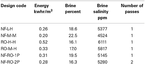
Table 3. Output technologies for irrigation (IMSDesign software).

To use the AHP, the decision-maker must specify his requirements (based on previous experience) for achieving the overall goal.

Model Implementation and Discussion

From the matrix obtained in Table 3, the geometric mean (w_i, approximately the product of the elements in each row regarding to a matrix of n rows and n columns) and the normalized geometric mean (p_i) are determined according to Equations (6) and (7), respectively.

$\begin{array}{cc}{w}_i={\left({\displaystyle \prod _{j=1}^n{a}_{ij}}\right)}^{1/n}i=1,\dots ,n& (6)\end{array}$

$\begin{array}{cc}{p}_i={\left({\displaystyle \prod _{i=1}^n{a}_{ij}}\right)}^{1/n}/{\displaystyle \sum _{i=1}^n{\left({\displaystyle \prod _{j=1}^n{a}_{ij}}\right)}^{1/n}}i=1,\dots ,n& (7)\end{array}$

where, a_ij is an evaluated value, i is the row index (alternative, i = 1,…, n) and j is the column index (quality attribute, j = 1,…, n). In Table 4 its shown that for each decision attribute chosen, the importance of the design options. It designates how the alternatives are preferred over others with respect to each objective as well as to the whole objective (Cay and Uyan, 2013).

TABLE 4

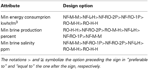
Table 4. Variability in importance across design options.

Table 5 compares minimization of energy consumption related to each of the options. One can see that according to the comparison the configurations NF-M-M is favorable (0.381). A comparable comparison was run for each of the attributes. The resultant set of weights for each of the option (in this case technology) with respect to each attributes is presented in Table 6.

TABLE 5

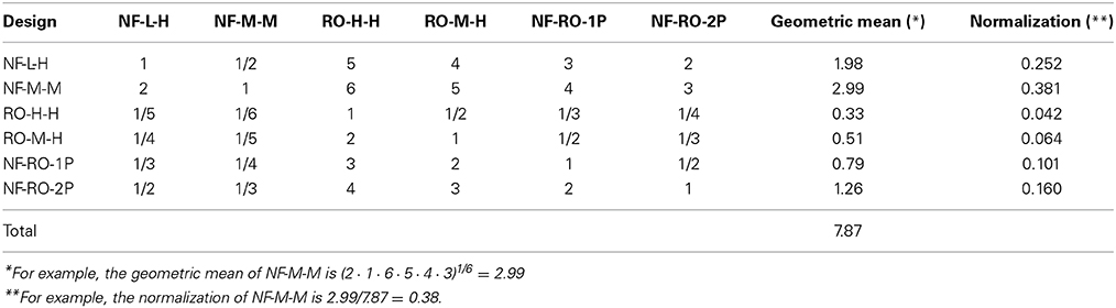
Table 5. AHP pair-wise evaluation of min energy consumption (Number are based on Saaty's Scale and an expert subjective point of view).

TABLE 6

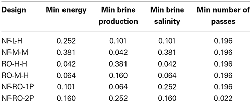
Table 6. AHP pair-wise results of attribute weights.

Discrepancies in the response assessments can occur and are related to human errors along the process. Let's assume that assumption A is preferred over assumption B and, assumption B is preferred over assumption C. Then, it can be assumed that assumption A should be preferred over assumption C by a wide margin. If throughout the pair-wise comparison A is vaguely preferred over C, then a contradiction is taken place. In this work, the statistics and implementation of a judgment matrix (Yang et al., 2013) was implemented.

Based on the results of the correlations between variables, the CoPlot diagram presented in Figure 2 shows “min brine salinity” and “min energy” relatively close to each other. “Min brine production”is pointing to the opposite direction and “min passes” is lying in-between. Consequently “min brine salinity”(or “min energy”) is identified as offering diminutive information and can be taken away from the analysis with no effect (or little effect) on the results. The results show that: NF-RO-2P is disconnected from the other units because it has the highest “min passes” value; RO-H-H is separated from the other units because it has the highest “min brine production” value; and NF-M-M is separated from the other units because it has the highest “min brine salinity”and “min energy” values. NF-RO-2P, RO-H-H and NF-M-M could be considered outliers (see Figure 2). Finally, NF-L-H is average in all variables and in conclusion appears quite near to the center-of-gravity, the point from which all arrows begin. It is being claimed in this paper that MDS can be used to present the result graphically, the lower value (min objective function) a unit gets, the more effective the design is assumed over that specific attribute and it is clearly shown (Figure 2) that the best configuration is achieved with NF-L-H.

FIGURE 2

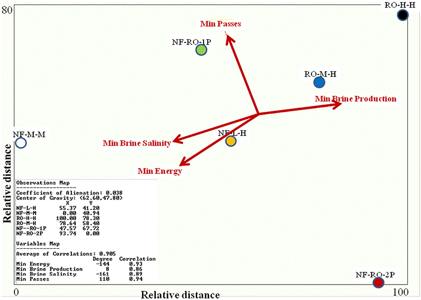
Figure 2. MDS map, generated by the proposed method (CoPlot): NF and RO configuration performance (at a permeate flux of 20 l/m²-h, six elements per vessel). Design: (i) one pass with ESNA1-LF-LD membranes (code NF-L-H); (ii) one pass with ESNA1-LF2-LD membranes (code NF-M-M); (iii) one pass with CPA5-MAX membranes (code RO-H-H); (iv) one pass with ESPA4-MAX membranes (code RO-M-H); (v) one pass with ESNA1-LF2-LD membranes at the first stage and ESPA4-MAX membranes at the second stage (code NF-RO-1P); and (vi) two pass with ESNA1-LF2-LD membranes at the first pass and ESPA4-MAX membranes at the second pass (code NF-RO-2P). Each variable is represented by an arrow, emerging from the center of gravity of the n points. The direction of each arrow is chosen so that the correlation between the actual values of the variable and their projections on the arrow is maximal. (MDS Statistics: “Coefficient of alienation” = 0.038, “Average of Correlations” = 0.905). The “goodness of fit” measures (concerning the “Coefficient of alienation” and the variables correlations) is satisfied both for the configurations and the variables.

The “goodness of fit” in the Coplot system is calculated by two types of measures: the “coefficient of alienation” (Θ) and the extend of the v maximal correlations that measure the “goodness of fit” of the j regressions. Smaller “coefficient of alienation” indicates better the output and, values lower than 0.15 are assumed precise. In this study (Figure 2) a coefficient of 0.038 is considered as an excellent figure. The “goodness of fit” of the j regressions helps to decide whether one eliminates or adds variables: Variables that do not fit into the graphical display, meaning, have low correlations, should be removed. Higher the variable's correlation, the better the variable's arrow represents common direction and order of the projections of the n points along the axis.

Based on this test case, the correlations of MDS data are high: average 0.905 (“min energy” = 0.93; “min brine production” = 0.86; “min brine salinity” = 0.89; “min passes” = 0.94). The two “goodness of fit” measurements (“coefficient of alienation” for the first step and four correlations for each one of the variables for the second step) allow the researchers to point out that according to this map the optimal solution is Nanofiltration technology (low rejection and high flux).

There are some limitations of these approaches: (i) Some problems are too complex resulting in a very complicated pair wise process that cannot be conducted by AHP and MDS, (ii) Not all individuals are capable in using and understanding the process; there is a need for experts, and (iii) The focus is on immediate technology impacts and not on the gain in substantial knowledge expertise and future improvements.

For the use of NF technology a reform of water pricing may be needed, which is most often driven by budget government pressure, rise of the costs of the services provided and, government aspiration to reduce subsidies. The World Bank has encouraged governments to employ a policy of cost recovery for many years, on the belief that users should cover O&M and some of the capital costs (Bustan et al., 2013).

The Public-Private Partnerships (PPP) can be viewed as the governance policy for minimizing transaction costs and; coordinating and enforcing relations between partners engaged in agricultural goods and services production. The Built Own and Operate (BOO) projects promotes an optimal policy tactic to enable social and economic development, bringing together competence, plasticity, and competence for the private sector with the responsibility, long-term outlook and social interest of the public sector (Johannessen et al., 2014).

The use of membrane technology in agriculture can lead to additional gains: (i) understanding the entire supply-chain instead of the bottlenecks, (ii) improved quality and quantity of sales' product, (iii) new market penetration, and (iv) positive social effects. Agricultural research concerning NF technology responds to multiple objectives. Clearness of objectives in determining water charges is vital and there are limits of valuing as a practical tool for irrigation demand. The authorities must take into consideration the environmental benefits by including incentives for appropriate water allocation and demand management.

Conclusions

Membrane technology selection for water treatment is often a subjective task: Combining quantitative methods into the evaluation procedure permits the decision makers to recognize the most suitable option in an objective and efficient way. In this study two methodologies were used and discussed to analyse multiple variable data:AHP and MDS (CoPlot).

The AHP method establishes an evaluation model for design of membrane technology based on IMSDesign software. Analysis results using Saaty's Scale indicates that the decision-makers may select the most appropriate option based on the following attributes: minimization of energy consumption, minimization of brine production, minimization of brine salinity, and minimization of design passes (investment cost).

Using the AHP method for assortment of optimal technology provides a systematically decision making a framework with several characteristics: (i) the performance of different technologies can be evaluated using multiple attributes—both quantitative and qualitative—rather than profitability alone; (ii) ratings allow to evaluate the use of the technologies for the end user; (iii) AHP method provides an effective way for managing process documentation; and (iv) the proposed method forms the basis for a intermittent process of planning and managing technology, so that the priorities of the technologies can easily be modified and updated.

AHP database is graphically introduced by the CoPlot technique, a multivariate statistical method that is remarkably robust and provides new insights about membrane configurations and design, giving a strong picture of what needs to be done next. The CoPlot technique provides a powerful analytic tool for brackish groundwater membrane system: the optimal configuration using AHP and MDS design is based on NF membrane (low rejection and high flux).

Conflict of Interest Statement

The authors declare that the research was conducted in the absence of any commercial or financial relationships that could be construed as a potential conflict of interest.

Acknowledgment

The research was funded by the Chief Scientist, Israeli Ministry of Agriculture and Rural Development (Project n. 459-4437-12).

References

Adler, N., and Raveh, A. (2008). Presenting DEA graphically. Omega 36, 715–729. doi: 10.1016/j.omega.2006.02.006

CrossRef Full Text | Google Scholar

Al-Amoudi, A., and Lovitt, R. W. (2007). Fouling strategies and the cleaning system of NF membranes and factors affecting cleaning efficiency. J. Membr. Sci. 303, 4–28. doi: 10.1016/j.memsci.2007.06.002

CrossRef Full Text | Google Scholar

Alghoul, M. A., Poovanaesvaran, P., Sopian, K., and Sulaiman, M. Y. (2009). Review of brackish water reverse osmosis (BWRO) system designs. Renew. Sust. Energ. Rev. 13, 2661–2667. doi: 10.1016/j.rser.2009.03.013

CrossRef Full Text | Google Scholar

Bartels, C., Hirose, M., and Fujioka, H. (2008). Performance advancement in the spiral wound RO/NF element design. Desalination 221, 207–214. doi: 10.1016/j.desal.2007.01.077

CrossRef Full Text | Google Scholar

Ben-Gal, A., Ityel, E., Dudley, L., Cohen, S., Yermiyahu, U., Presnov, E., et al. (2008). Effect of irrigation water salinity on transpiration and on leaching requirements: a case study for bell peppers. Agric. Water Manage. 95, 587–597. doi: 10.1016/j.agwat.2007.12.008

CrossRef Full Text | Google Scholar

Bernstein, N., Ioffe, M., Luria, G., Bruner, M., Nishri, Y., Philosoph-Hadad, S., et al. (2011). Effects of K and N nutrition on function and production of Ranunculus asiaticus. Pedosphere 21, 288–301. doi: 10.1016/S1002-0160(11)60129-X

CrossRef Full Text | Google Scholar

Bick, A., Gillerman, L., Manor, Y., and Oron, G. (2012). Economic assessment of an integrated membrane system for secondary effluent polishing for unrestricted reuse. Water 4, 219–236. doi: 10.3390/w4010219

Pubmed Abstract | Pubmed Full Text | CrossRef Full Text | Google Scholar

Bick, A., Yang, F., Shandalov, S., Raveh, A., and Oron, G. (2011). Multi-dimension scaling as an exploratory tool in the analysis of an immersed membrane bioreactor. Membr. Water Treat. 2, 105–119. doi: 10.12989/mwt.2011.2.2.105

CrossRef Full Text

Birnhack, L., Shlesinger, N., and Lahav, O. (2010). A cost effective method for improving the quality of inland desalinated brackish water destined for agricultural irrigation. Desalination 262, 152–160. doi: 10.1016/j.desal.2010.05.061

CrossRef Full Text | Google Scholar

Bozoki, S., Fulop, J., and Koczkodaj, W. W. (2011). An LP-based inconsistency monitoring of pairwise comparison matrices. Math. Comput. Model. 54, 789–793. doi: 10.1016/j.mcm.2011.03.026

CrossRef Full Text | Google Scholar

Bravata, D. M., Shojania, K. G., Olkin, I., and Raveh, A. (2008). CoPlot: a tool for visualizing multivariate data in medicine. Stat. Med. 27, 2234–2247. doi: 10.1002/sim.3078

Pubmed Abstract | Pubmed Full Text | CrossRef Full Text | Google Scholar

Bui, E. N. (2013). Soil salinity: a neglected factor in plant ecology and biogeography. J. Arid Environ. 92, 14–25. doi: 10.1016/j.jaridenv.2012.12.014

CrossRef Full Text | Google Scholar

Bustan, A., Avni, A., Yermiyahu, U., Ben-Gal, A., Riov, J., Erel, R., et al. (2013). Interactions between fruit load and macroelement concentrations in fertigated olive (Olea europaea L.). trees under arid saline conditions. Sci. Hortic. 152, 44–55. doi: 10.1016/j.scienta.2013.01.013

CrossRef Full Text | Google Scholar

Caputo, A. C., Pelagagge, P. M., and Salini, P. (2013). AHP-based methodology for selecting safety devices of industrial machinery. Saf. Sci. 53, 202–218. doi: 10.1016/j.ssci.2012.10.006

CrossRef Full Text | Google Scholar

Cay, T., and Uyan, M. (2013). Evaluation of reallocation criteria in land consolidation studies using the Analytic Hierarchy Process (AHP). Land Use Policy 30, 541–548. doi: 10.1016/j.landusepol.2012.04.023

CrossRef Full Text | Google Scholar

Chakrabortty, S., Roy, M., and Pal, P. (2013). Removal of fluoride from contaminated groundwater by cross flow nanofiltration: transport modelling and economic evaluation. Desalination 313, 115–124. doi: 10.1016/j.desal.2012.12.021

CrossRef Full Text | Google Scholar

Connor, J. D., Schwabe, K., King, D., and Knapp, K. (2012). Irrigated agriculture and climate change: the influence of water supply variability and salinity on adaptation. Ecol. Econ. 77, 149–157. doi: 10.1016/j.ecolecon.2012.02.021

CrossRef Full Text | Google Scholar

Edelstein, M., Plaut, Z., Dudai, N., and Ben-Hur, M. (2009). Vetiver (Vetiveria zizanioides) responses to fertilization and salinity under irrigation conditions. J. Environ. Manage. 91, 215–221. doi: 10.1016/j.jenvman.2009.08.006

Pubmed Abstract | Pubmed Full Text | CrossRef Full Text | Google Scholar

Garcia, N., Moreno, J., Cartmell, E., Rodriguez-Roda, I., and Judd, S. (2013). The cost and performance of an MF-RO/NF plant for trace metal removal. Desalination 309, 181–186. doi: 10.1016/j.desal.2012.10.017

CrossRef Full Text | Google Scholar

Ghermandi, A., and Mesalem, R. (2009). The advantages of NF desalination of brackish water for sustainable irrigation: the case of the Arava Valley in Israel. Desalination Water Treat. 10, 101–107. doi: 10.5004/dwt.2009.824

CrossRef Full Text | Google Scholar

Gomez-Silvan, C., Arevalo, J., Perez, J., Gonzalez-Lopez, J., and Rodelas, B. (2013). Linking hydrolytic activities to variables influencing a submerged membrane bioreactor (MBR) treating urban wastewater under real operating conditions. Water Res. 47, 66–78. doi: 10.1016/j.watres.2012.09.032

Pubmed Abstract | Pubmed Full Text | CrossRef Full Text | Google Scholar

Gur-Reznik, S., Koren-Menashe, I., Heller-Grossman, L., Rufel, O., and Dosoretz, C. G. (2011). Influence of seasonal and operating conditions on the rejection of pharmaceutical active compounds by RO and NF membranes. Desalination 277, 250–256. doi: 10.1016/j.desal.2011.04.029

CrossRef Full Text | Google Scholar

Gursoy, B. B., Mason, O., and Sergeev, S. (2013). The analytic hierarchy process, max algebra and multi-objective optimisation. Linear Algebra Appl. 438, 2911–2928. doi: 10.1016/j.laa.2012.11.020

CrossRef Full Text | Google Scholar

Gutman, J., Fox, S., and Gilron, J. (2012). Interactions between biofilms and NF/RO flux and their implications for control-a review of recent developments. J. Membr. Sci. 421–422, 1–7. doi: 10.1016/j.memsci.2012.06.032

CrossRef Full Text | Google Scholar

Guttman, L. (1968). A general non-metric technique for finding the smallest space for a configuration of points. Psychometrica 33, 479–506.

Google Scholar

Hilal, N., Al-Zoubi, H., Darwish, N. A., and Mohammad, A. W. (2005). Characterisation of nanofiltration membranes using atomic force microscopy. Desalination 177, 187–199. doi: 10.1016/j.desal.2004.12.008

CrossRef Full Text | Google Scholar

Hillel, D., Belhassen, Y., and Shani, A. (2013). What makes a gastronomic destination attractive? Evidence from the Israeli Negev. Tourism Manage. 36, 200–209. doi: 10.1016/j.tourman.2012.12.006

CrossRef Full Text | Google Scholar

Johannessen, A., Rosemarin, A., Thomalla, F., Swartling, A. G., Stenström, T. A., Vulturius, G., et al. (2014). Strategies for building resilience to hazards in water, sanitation and hygiene (WASH) systems: the role of public private partnerships. Int. J. Disaster Risk Reduct. 10, 102–115. doi: 10.1016/j.ijdrr.2014.07.002

CrossRef Full Text | Google Scholar

Karabelas, A. J., Koutsou, C. P., Gragopoulos, J., Isaias, N. P., and Al Rammah, A. S. (2012). A novel system for continuous monitoring of salt rejection characteristics of individual membrane elements in desalination plants. Sep. Pur. Technol. 88, 29–38. doi: 10.1016/j.seppur.2011.12.002

CrossRef Full Text | Google Scholar

Kayastha, P., Dhital, M. R., and De Smedt, F. (2013). Application of the analytical hierarchy process (AHP). for landslide susceptibility mapping: a case study from the Tinau watershed, west Nepal. Comput. Geosci. 52, 398–408. doi: 10.1016/j.cageo.2012.11.003

CrossRef Full Text | Google Scholar

Lespinats, S., Fertil, B., Villemain, P., and Herault, J. (2009). RankVisu: mapping from the neighborhood network. Neurocomputing 72, 2964–2978. doi: 10.1016/j.neucom.2009.04.008

CrossRef Full Text | Google Scholar

Levy, D., and Tai, G. C. C. (2013). Differential response of potatoes (Solanum tuberosum L.) to salinity in an arid environment and field performance of the seed tubers grown with fresh water in the following season. Agric. Water Manage. 116, 122–127. doi: 10.1016/j.agwat.2012.06.022

CrossRef Full Text | Google Scholar

Lew, B., Cochva, M., and Lahav, O. (2009). Potential effects of desalinated water quality on the operation stability of wastewater treatment plants. Sci. Total Environ. 407, 2404–2410. doi: 10.1016/j.scitotenv.2008.12.023

Pubmed Abstract | Pubmed Full Text | CrossRef Full Text | Google Scholar

Lipshitz, G., and Raveh, A. (1994). Applications of the CoPlot method in the study of socioeconomic differences among cities: a basis for a differential development policy. Urban Stud. 31, 123–135.

Google Scholar

Liu, Y., Li, X., Xing, Z., Zhao, X., and Pan, Y. (2013). Responses of soil microbial biomass and community composition to biological soil crusts in the revegetated areas of the Tengger Desert, Appl. Soil Ecol. 65, 52–59. doi: 10.1016/j.apsoil.2013.01.005

CrossRef Full Text | Google Scholar

Miller, G. W. (2006). Integrated concepts in water reuse: managing global water needs. Desalination 187, 65–75. doi: 10.1016/j.desal.2005.04.068

CrossRef Full Text | Google Scholar

Mrayed, S. M., Sanciolo, P., Zou, I., and Leslie, G. (2011). An alternative membrane treatment process to produce low-salt and high-nutrient recycled water suitable for irrigation purposes. Desalination 274, 144–149. doi: 10.1016/j.desal.2011.02.003

CrossRef Full Text | Google Scholar

Nederlof, M. M., van Paassen, J. A. M., and Jong, R. (2005). Nanofiltration concentrate disposal: experiences in the Netherlands. Desalination 178, 303–312. doi: 10.1016/j.desal.2004.11.041

CrossRef Full Text | Google Scholar

Oren, S., Birnhack, L., Lehmann, O., and Lahav, O. (2012). A different approach for brackish-water desalination, comprising acidification of the feed-water and CO₂(aq). reuse for alkalinity, Ca²⁺ and Mg²⁺ supply in the post treatment stage. Sep. Purif. Technol. 89, 252–260. doi: 10.1016/j.seppur.2012.01.027

CrossRef Full Text | Google Scholar

Oron, G., Gillerman, L., Bick, A., Manor, Y., Buriakovsky, N., and Hagin, J. (2008). Membrane technology for sustainable treated wastewater reuse: agricultural, environmental and hydrological considerations. Water Sci. Technol. 57, 1383–1388. doi: 10.2166/wst.2008.243

Pubmed Abstract | Pubmed Full Text | CrossRef Full Text | Google Scholar

Penate, B., and García-Rodríguez, L. (2011). Reverse osmosis hybrid membrane inter-stage design: a comparative performance assessment. Desalination 281, 354–363. doi: 10.1016/j.desal.2011.08.010

CrossRef Full Text | Google Scholar

Qadir, M., Sharma, B. R., Bruggeman, A., Choukr-Allah, R., and Karajeh, F. (2007). Non-conventional water resources and opportunities for water augmentation to achieve food security in water scarce countries. Agric. Water Manage. 87, 2–22. doi: 10.1016/j.agwat.2006.03.018

CrossRef Full Text | Google Scholar

Rasouli, F., Pouya, A. K., and Karimian, N. (2013). Wheat yield and physico-chemical properties of a sodic soil from semi-arid area of Iran as affected by applied gypsum. Geoderma 193–194, 246–255. doi: 10.1016/j.geoderma.2012.10.001

CrossRef Full Text | Google Scholar

Raveh, A. (2000). CoPlot: a Graphic display method for geometrical representations of MCDM. Eur. J. Oper. Res. 125, 670–678. doi: 10.1016/S0377-2217(99)00276-3

CrossRef Full Text | Google Scholar

Riera, F. A., Suarez, A., and Muro, C. (2013). Nanofiltration of UHT flash cooler condensates from a dairy factory: Characterisation and water reuse potential. Desalination 309, 52–63. doi: 10.1016/j.desal.2012.09.016

CrossRef Full Text | Google Scholar

Saaty, T. L. (1980). The Analytic Hierarchy Process. New York, NY: McGraw-Hill.

Saaty, T. L. (2003). Decision-making with the AHP: why is the principal eigenvector necessary. Eur. J. Oper. Res. 145, 85–91. doi: 10.1016/S0377-2217(02)00227-8

CrossRef Full Text | Google Scholar

Schilli, C., Lischeid, G., and Rinklebe, J. (2010). Which processes prevail?: analyzing long-term soil solution monitoring data using nonlinear statistics. Geoderma 158, 412–420. doi: 10.1016/j.geoderma.2010.06.014

CrossRef Full Text | Google Scholar

Sotto, A., Arsuaga, J. M., and Van der Bruggen, B. (2013). Sorption of phenolic compounds on NF/RO membrane surfaces: Influence on membrane performance. Desalination 309, 64–73. doi: 10.1016/j.desal.2012.09.023

CrossRef Full Text | Google Scholar

Tzfati, E., Sein, M., Rubinov, A., Raveh, A., and Bick, A. (2011). Pre-treatment of wastewater: optimal coagulant selection using partial order scaling analysis (POSA). J. Hazard Mater. 190, 51–59. doi: 10.1016/j.jhazmat.2011.02.023

Pubmed Abstract | Pubmed Full Text | CrossRef Full Text | Google Scholar

Yermiyahu, U., Tal, A., Ben-Gal, A., Bar-Tal, J., and Tarchitzky, O. (2007). Lahav, rethinking desalinated water quality and agriculture. Science 318, 920–921. doi: 10.1126/science.1146339

Pubmed Abstract | Pubmed Full Text | CrossRef Full Text | Google Scholar

Verhuelsdonk, M., Attenborough, T., Lex, O., and Altmann, T. (2010). Design and optimization of seawater reverse osmosis desalination plants using special simulation software. Desalination 250, 729–733. doi: 10.1016/j.desal.2008.11.031

CrossRef Full Text | Google Scholar

Villarreal-Guerrero, F., Kacira, M., Fitz-Rodríguez, E., Kubota, C., Giacomelli, G. A., Linker, R., et al. (2012). Comparison of three evapotranspiration models for a greenhouse cooling strategy with natural ventilation and variable high pressure fogging. Sci. Hortic. 134, 210–221. doi: 10.1016/j.scienta.2011.10.016

CrossRef Full Text | Google Scholar

Vince, F., Marechal, F., Aoustin, E., and Breant, P. (2008). Multi-objective optimization of RO desalination plants. Desalination 222, 96–118. doi: 10.1016/j.desal.2007.02.064

CrossRef Full Text | Google Scholar

Wei, J., Qiu, C., Wang, Y. N., Wang, R., and Tang, C. Y. (2013). Comparison of NF-like and RO-like thin film composite osmotically-driven membranes-Implications for membrane selection and process optimization, J. Membrane Sci. 427, 460–471. doi: 10.1016/j.memsci.2012.08.053

CrossRef Full Text | Google Scholar

Yang, X., Yan, L., and Zeng, L. (2013). How to handle uncertainties in AHP: The cloud delphi hierarchical analysis. Inform. Sci. 222, 384–404. doi: 10.1016/j.ins.2012.08.019

CrossRef Full Text | Google Scholar

Zhang, R., Zhang, X., Yang, J., and Yuan, H. (2013). Wetland ecosystem stability evaluation by using analytical hierarchy process (AHP) approach in Yinchuan Plain, China. Math. Comput. Model. 57, 366–374. doi: 10.1016/j.mcm.2012.06.014

CrossRef Full Text | Google Scholar

Zhao, S., Zou, L., and Mulcahy, D. (2012). Brackish water desalination by a hybrid forward osmosis–nanofiltration system using divalent draw solute. Desalination 284, 175–181. doi: 10.1016/j.desal.2011.08.053

CrossRef Full Text | Google Scholar

Zheng, Y., Yu, S., Shuai, S., Zhou, Q., Cheng, Q., Liu, M., et al. (2013). Color removal and COD reduction of biologically treated textile effluent through submerged filtration using hollow fiber nanofiltration membrane. Desalination 314, 89–95. doi: 10.1016/j.desal.2013.01.004

CrossRef Full Text | Google Scholar

Zhou, F., Wang, C., and Wei, J. (2013). Separation of acetic acid from monosaccharides by NF and RO membranes: performance comparison. J. Membr. Sci. 429, 243–251. doi: 10.1016/j.memsci.2012.11.043

CrossRef Full Text | Google Scholar