Parametric linear hybrid automata for complex environmental systems modeling

1. Introduction

1.1. Environmental Systems

Environmental systems are a broad category of systems which interact or have an impact on the environment. These systems can range from different chemical processes found in nature to large scale interactions between different biotic and abiotic factors, as represented in the modeling studies of Lake Balaton (Somlydy, 1982; Ttrai et al., 2000). In contrast to more traditional systems, as studied in other physical sciences, environmental systems are tightly integrated with each other, forming different sub-domains within each system (Hanrahan, 2010). As such, they are difficult to study in isolation since their behavior changes with respect to other environmental factors working in conjunction with each other (Hanrahan, 2010).

1.2. Modeling of Environmental Systems

Because of their broad spectrum, different approaches have been employed in the modeling and analysis of environmental systems over the years. The approaches can be grouped into stochastic and probabilistic (Refsgaard et al., 2007; Gottschalk et al., 2010; Sun et al., 2014), statistical (Refsgaard et al., 2007; Uusitalo, 2007; Berie, 2014), differential (Casulli and Zanolli, 2002; Coulthard et al., 2005; Hanrahan, 2010), or a combinations of these methodologies. In recent years, different artificial intelligence (AI) approaches have also been applied, such as machine learning (Wiley et al., 2003; Kanevski et al., 2004) and agent based modeling (Sengupta and Bennett, 2003; Crooks et al., 2008). However, certain aspects of the system elude these approaches, such as the larger view of the behaviors of the system–statistical methods do not represent the dynamics of the system, probabilistic approaches lack deterministic predictability, and differential and AI models suffer from high levels of complexity when modeling realistic parameters.

1.3. Our Contribution

In this paper, we present a hybrid modeling approach using linear hybrid automata for the behavioral modeling of the system. We have already applied this approach in the domain of systems biology, particularly in the modeling of biological regulatory networks (Ahmad et al., 2012; Aslam et al., 2014). The advantage of this approach is that it allows the modeling of large regulatory systems, assisting in the inference of the dynamics of the system, without having to deal with the exact rates or parameters governing the said system. To demonstrate our approach, we have applied our framework on two case studies, a microbial system in a freshwater pond, and a slightly more complex atmospheric system (adapted from Seppelt, 2007), explained below. For the sake of readability, the given examples only deal with a small number of components, but the presented methods are applicable on larger systems as well.

1.4. Case Study 1: Microbial Population

Consider the microbial populations of three particular microbes in a freshwater pond. The first of these microbes, labeled M1, generates a certain product which acts as a nutrient for the second microbe, labeled M2. However, the microbe M2 produces a toxin which is harmful to the first microbe, M1. Apart from the toxin, the microbe M2 also produces a nutrient for the third microbe, M3. The third microbe acts as a dominant predator instead, and generates a toxin which is harmful to both the first microbe, M1, and the second microbe M2. However, in order to sustain itself, the third microbe can also produce its own nutrients, but only when it is present in sufficient numbers to form colonies.

1.5. Case Study 2: Atmospheric System

Consider a slightly simplified version of the atmosphere, particularly pertaining to the interconnectedness of the temperature of the planet and the water cycle. Whenever the sun shines, it increases the temperature, and makes evaporation possible (provided that there is a source of water available). As the temperature increases and the water evaporates, clouds begin to form which can produce two effects: (i) the sun gets blocked, lowering the temperature; and (ii) precipitation is produced which resupplies the water sources for future evaporation. However, persistent high temperatures can increase the air temperature, blocking condensation, and cloud formation. Likewise, persistent evaporation without precipitation can drain the available water source(s).

1.6. Plan of the Paper

We begin with the Methodology Section where we describe the work flow of our approach, the formalisms and frameworks used, and its step by step application on Case Study 1. Following it is the Results Section in which we apply the given methodology on Case Study 2, ending with the Discussion Section where we discuss the applicability of our approach, its advantages, and its disadvantages. A list of glossary items containing technical terms and their short descriptions are also provided at the end of this article (Table A1).

2. Methodology

Our methodology focuses on building an initial discrete model of the system in question, using the Kinetic Modeling formalism set forth by Kauffman in the late 1960s (Kauffman, 1969) and then by Thomas in the late 1970s (Thomas, 1978, 1979, 1998; Thomas et al., 1995) for biological regulatory networks. The basic idea of the approach was that natural phenomena are often observable when there is a switch from a relatively stable mode to another different mode.

This approach appeals for discrete modeling with states and transitions where time elapses in the states and transitions between these states are instantaneous. The important data being the time spent in one state whatever the evolution in this state actually is, abstraction can then be done in order to take into account lengthening actions besides almost infinitely fast switches. This stands for the hybrid feature. Thus, a discrete model allows us to observe the dynamics of the system, in the form of a state graph, using arbitrary discrete values to represent different levels of activities each entity or object can exhibit. Once the discrete dynamics of the system are obtained, Parametric Biological Linear Hybrid Automata (Bio-LHA, Ahmad et al., 2006; Ahmad, 2009) can be constructed on targeted trajectories to isolate conjuncted parametric delay constraints governing these trajectories (Ahmad et al., 2007, 2008; Ahmad and Roux, 2010). These delays assist us in inferring different temporal constraints a system must follow to generate the specified trajectory, and which constraints can be targeted to destabilize the said trajectory. The whole process is represented in Figure 1 and can be broken into the following steps:

• The pathways pertaining to the system are extracted from the literature and abstracted to the form of a discrete regulatory network. These pathways can comprise of simple linear processes to complex and dense interactions such as feedbacks, feed forward loops, branching processes etc.

• The regulatory network then undergoes model checking to generate sets of logical parameters which satisfy particular system specific observations extracted from the literature.

• The parameters are loaded into the regulatory network to generate discrete dynamics of the system (also called discrete state space), represented as a directed state graph.

• Network analysis, in particular the shortest path betweenness centrality calculation, is conducted for each state of the state graph to isolate specific trajectories comprising of states satisfying particular centrality constraints.

• The isolated trajectories are then converted to respective Bio-LHAs which are then used to find the delay constraints in the form of path constraints (for acyclic trajectories), invariance kernels (for cyclic trajectories), or convergence domains (for asymptotic trajectories).

• These constraints are then refined to form pairwise relations between the respective parameters governing the activation or inhibition delay of the involved entities.

FIGURE 1

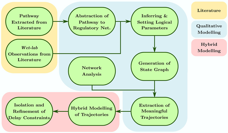
Figure 1. The work-flow of the methodology applied in this study.

In order to properly understand the requirements and application of the approach, we detail the mathematical definitions and their application on Case Study 1 (Microbial population) in the following subsections.

2.1. Discrete Modeling

The formal definitions of the René Thomas kinetic logic formalism, adapted from Thomas (1979), Thomas and d'Ari (1990), Ahmad et al. (2012), and Paracha et al. (2014), are provided below:

Definition 1. [Regulatory Network]. A directed graph G = (V, E) is a regulatory network (RN) when,

• V, with a typical element v, is the set of vertexes,

• E, with a typical element e = (v_m, v_n), is the set of edges directed from a source vertex v_m to the target vertex v_n,

• G⁺(v) represents the set of the targets of the vertex v, while G⁻(v) represents the set of its sources,

• each edge is labeled by the pair (j_vm, v_n, η_{vm, vn}) such that j_{vm, vn} is the positive integer representing the concentration level required for the interaction, and η_{vm, vn} ∈ {+, −} shows the type of interaction with ‘+’ being activation and ‘−’ being inhibition,

• ∀v_n ∈ G⁺ (v_m), each j_{vm, vn} ∈ {1, 2, …, max_vm} where max_vm is less than or equal to the number of vertexes in G⁺ (v_m),

• each v ∈ V has a set Z_v = {0, 1, …, max_v} representing its discrete abstracted concentration levels.

Figure 2 shows the regulatory network of Case Study 1. Here the set V = {M1, M2, M3} is the set of vertexes, representing the three entities (discretized populations of microbes), and E = {(M1, M2), (M2, M1), (M2, M3), (M3, M2), (M3, M1), (M3, M3)} is the set of edges, each labeled with a positive integer and sign. For example, the edge e = (M2, M3) has j_{M2, M3} = 1 and η_{M2, M3} = “+.” The integer represents the level of the source entity required to perform the action, whereas the sign shows the type of action: “+” for activation and “−” for inhibition. Thus, the source entity for “+” is the activator, and for “−” the inhibitor. Furthermore, continuing the example, the vertex M3 has max_M3 ≤ 3 as G⁺(M3) = {M1, M2, M3}. Likewise, G⁻(M3) = {M2, M3}.

FIGURE 2

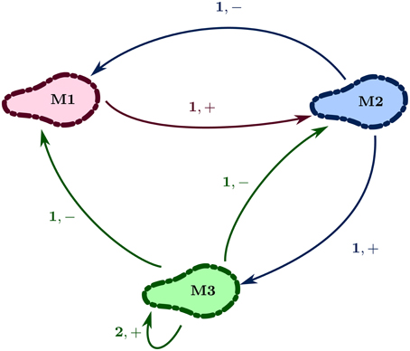
Figure 2. Regulatory network of Case Study 1: Microbial population.

Components of a RN are autonomous processes, with each having different values (discrete abstracted concentration levels) and variables depending upon the interactions with the other components in the dynamic system. At each moment, the whole system is in a given state represented by the tuple formed by the values of each component. In order to understand the dynamics of the discrete model, the states of the regulatory network and the resources and logical parameters of each entity in the respective state are formally defined as,

Definition 2. [State]. A state of an RN is an ordered tuple of the discrete levels of each entity represented as (s_xv)_∀v∈V ∈ S where,

• S = Π_v∈VZ_v is the set of all states, and

• x_v ∈ Z_v represents the discrete level of the entity v ∈ V.

Thus, a state labeled “102,” representing the state (1, 0, 2) for Case Study 1 RN (Figure 2), would represent the discrete levels as M1 = 1, M2 = 0, M3 = 2, in that order.

The resources of one component stand for the set of the components (possibly including itself) that are positively acting on it at the moment. This is again dynamic since it depends on the current value of each of the components, as well as their interactions with the given component. Formally,

Definition 3. [Resources]. For a given state of an RN, the resource set Q_xvn for an entity v_n ∈ V at concentration level x_vn is defined as Q_xvn = {v_m ∈ G⁻(v_n)|(x_vm ≥ j_{vm, vn} ∧ η_{vm, vn}=‘+’)⊗(x_vm < j_{vm, vn} ∧ η_{vm, vn}=‘−’)}.

For the state (1, 0, 2), the resource set Q_1M1 is {M2} as M2 cannot inhibit it below its respective discrete level “1” while M3 is inhibiting it above its respective level “2,” Q_0M2 is {M1} as M1 is activating it at level “1,” and Q_2M3 is {M3} as M3 is a self-activator at level “2.”

Definition 4. [Logical Parameters]. The set of logical parameters of an RN “G” is defined as K(G) = {K_vm(Q_xvm) ∈ Z_vm ∀ v_m ∈ V}.

The meaning of the logical parameters is that it defines the discrete level that the entity will evolve toward, given the set of resources for the entity available. So, for example, if the parameter K_M2{M1} is set to “0” (meaning that in the presence of both M1 and M3, the microbe M2 will still decline in population) then the level M2 will evolve toward “0” through a step function, similar to the those shown in Figure 3.

FIGURE 3

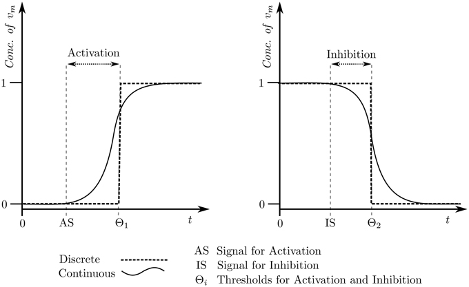
Figure 3. Discrete approximation of the continuous evolution pertaining to concentration of an entity.

The parameter K_vm governs the evolution of the entity v_m via the evolution operator “↱” (Bernot et al., 2004) against the rule:

$x_{v_m}\Rsh K_{v_m}(Q_{x_{v_m}})=\{\begin{array}{ll}{x}_{v_m}+1\hfill & if\text{}{x}_{v_m}<K_{v_m}(Q_{x_{v_m}});\hfill \\ x_{v_m}\hfill & if\text{}{x}_{v_m}=K_{v_m}(Q_{x_{v_m}});\hfill \\ x_{v_m}-1\hfill & if\text{}{x}_{v_m}>K_{v_m}(Q_{x_{v_m}}).\hfill \end{array}$

Table 1 shows all the logical parameters of Case Study 1. As a general rule, when only the activators of an entity v are present then the respective entity approaches its max_v, whereas when only the inhibitors are present then it approaches “0.” Both of these cases are termed as trivial parameters. Once selected, the logical parameters are then plugged into the respective RN, generating a new directed graph reflecting the discrete dynamics of the system, formally defined as:

TABLE 1

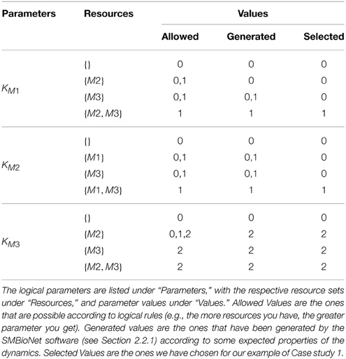
Table 1. Case Study 1: Parameter table.

Definition 5. [State Graph]. The state graph of an RN is a directed graph SG = (S, T) where,

• S is the set of states as defined in Definition 2, and

• T ⊆ S × S is the set of unlabeled edges representing transitions between states such that for each ordered transition s → s′, ∃ v_m ∈ V such that s_xvm ≠ s′_xvm, s′_xvm = s_xvm ↱ K_vm(Q_xvm), and ∀ v_n ∈ V \ {v_m}, s_xvn = s′_xvn.

In summary, each state of the state graph will differ from the other states in at least one entity level. The transitions between the states, on the other hand, will be defined by the logical parameters and available resources of the entities, and will have a target state differing from the source state in exactly one entity level. Figure 4 shows the state graph of Case Study 1 using the logical parameter set given in the “Selected” column in Table 1. As an example, the state transition (1, 0, 0) → (1, 1, 0) differs in the level of M2 only, and is only possible because of the logical parameter K_M2{M1, M3} = 1. Using the state graph individual behaviors of the system can be studied in the form of trajectories, formally defined as:

FIGURE 4

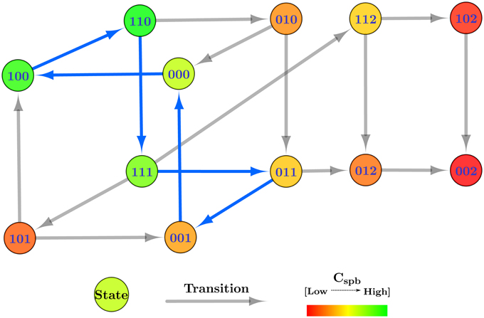
Figure 4. Centrality applied state graph of Case Study 1: Microbial population. The cycle selected for hybrid modeling is shown via blue state transitions.

Definition 6. [Trajectory]. A trajectory is defined as a successive series of transitions in a state graph.

Cyclic trajectories, representing oscillatory behavior, always end up in the starting state s_i ∈ S, whereas acyclic trajectories end at any state other than the starting (s_n ≠ s_i). A divergent trajectory shares transitions up to a certain extent with another trajectory, and then takes different transitions to different states. The length of the trajectory equals the total number of transitions in the said trajectory. The state graph can also be used to explain deadlocked states as states which do not have any transitions to other states. In practice, such states usually represent configurations of the system which are not favorable in terms of behavior. In Figure 4, the state (0, 0, 2) is the deadlock and represents the domination of the microbe M3 over the other two species.

2.2. Optimization of Discrete Modeling

2.2.1. Model Checking

As mentioned earlier in this section, the Hybrid Modeling targets specific trajectories of the RN, present in its state graph. However, the state graph contains many trajectories, and is dependent on a specific set of logical parameters. Table 1 shows different values that are allowed for each of the logical parameter, with each possible set generating different state graphs and behaviors. Bernot et al. (2004) pioneered an application of automated model checking, specifically Computation Tree Logic (CTL), to select particular sets of logical parameters for discrete modeling. Model checking is an exhaustive automated computational technique which is used to verify different properties in a given system (Clarke et al., 1999). In the SMBioNet software (Bernot et al., 2004; Khalis et al., 2009), the system is provided in the form of an RN, and the observations or known behaviors of the system are encoded in CTL. The software then checks all logical parameters to find and select the ones which can generate the encoded observations.

For Case Study 1, two observations were selected for the screening of logical parameters: from an arbitrary starting state (1, 0, 0), (i) there should exist at least one trajectory which will return to this state to form a cycle, and (ii) there should be at least one trajectory which will end up in the deadlock. Using the general rule of logical parameters described in Section 2.1 after Definition 4 (“Allowed” column in Table 1), coupled with the above observations in CTL, SMBioNet generated eight possible logical parameter sets, shown under the “Generated” column in Table 1. A single set is then selected from these generated values, given under the “Selected” column, which is then plugged into the RN. The source file used for the generation of these sets is provided in the Supplementary Materials file. Details of SMBioNet and CTL can be studied in-depth in the excellent review article by Khalis et al. (2009).

2.2.2. Network Analysis

A state graph of a particular system may contain any number of trajectories, depending on the number of entities and the state transitions, which makes the behavior of the system non-deterministic between the said trajectories. As such, selecting specific trajectories for hybrid modeling becomes difficult, especially in the absence of available observations. To assist in the selection of trajectories, we employ a network analysis technique, shortest path betweenness centrality analysis, to isolate trajectories. Adapted from Juncker and Schreiber (2008),

Definition 7. [Shortest Path Betweenness Centrality]. The shortest path betweenness centrality (C_spb), also defined as betweenness centrality, measures the occurrence of the a particular vertex v ∈ V in all the shortest paths between other vertexes. Mathematically, it is computed as $C_{spb}={\displaystyle {\sum }_{p\ne q\ne r\in S}\frac{{\sigma }_{pr}(q)}{{\sigma }_{pr}}}$ where,

• σ_pr is the total number of shortest trajectories from the state p to r, and

• σ_pr(q) is the total number of shortest trajectories from p to r which pass through q.

In short, C_spb measures the frequency of the occurrences of each state in the trajectories between other states, and as a fraction, only ranges from “0” to “1.” This allows for a relative measure of the states amongst themselves, with states having C_spb of at or near “1” occurring more frequently in the dynamics and trajectories of the system, than states which have their C_spb at or near “0.” The significance of this measure also increases with the fact that C_spb of deadlock states automatically becomes zero because all trajectories get stuck in the deadlock state and do not pass through it to reach any other state. This reflects the tendency of oscillating systems to avoid deadlocked states. In comparison to other centrality analyses available in the field of network analysis, C_spb is the only measure which is able to cater to both of these properties simultaneously. For example, closeness centrality measure (Juncker and Schreiber, 2008) caters to lower numerical values for deadlocked states, but does not cater to the relevance of the states themselves in terms of cyclic trajectories, thus not solving non-determinism. Likewise, the eccentricity centrality will represent the overall reachability of a particular state from other states, but will not contribute toward the solution of non-determinism in terms of selecting preferred trajectories in the system.

The table containing the C_spb of each state of the state graph for Case Study 1 is provided in the Supplementary Materials file, and Figure 4 is color coded to reflect higher measures of C_spb with green, and lower levels with red. For this case study, a cyclic trajectory comprising of the states with the highest centralities was selected for hybrid modeling, as this would theoretically reflect the most favorable and most probable behavior of the system based on the frequent occurrences of the constituent states. We begin with the state with the highest C_spb, in this case state (1, 1, 0), and select the state with the highest centrality from its target states, in this case (1, 1, 1). We then select the state with the highest centrality from the targets of (1, 1, 1), which is (0, 1, 1). Continuing onwards, the trajectory builds toward the state (0, 0, 1), (0, 0, 0), (1, 0, 0), and finally back to the starting state (1, 1, 0), completing a cycle with the highest cumulative C_spb. This cycle, (1, 1, 0) → (1, 1, 1) → (0, 1, 1) → (0, 0, 1) → (0, 0, 0) → (1, 0, 0) → (1, 1, 0), is represented in Figure 4 via blue transitions between the states.

2.3. Hybrid Modeling

As mentioned earlier in this section, the hybrid model is constructed on particular trajectories of the state graph. In the approach we use the Parametric Biological Linear Hybrid Automata (Bio-LHA) to convert the selected trajectory into a hybrid model by merging the constructed discrete system with time constraints. The formal definition of Bio-LHA, adapted from Ahmad et al. (2007); Ahmad and Roux (2010) is given below.

Let C⁼(X, P), C^≤(X, P), and C^≥(X, P) be the set of constraints using only =, ≤, and ≥, respectively. Here, X and P are the sets of real valued variables and parameters, respectively.

Definition 8. [Parametric Bio Linear Hybrid Automaton (Bio-LHA)]. A parametric bio linear hybrid automaton 𝔹 is a tuple (L, l₀, X, P, E, Inv, Dif) where,

• L is a finite set of locations,

• l₀ ∈ L is the initial location,

• P is a finite set of parameters (delays),

• X is a finite set of real-valued variable (clocks),

• E ⊆ L × C⁼(X, P) × 2^X × L is a finite set of edges with typical element e = (l, g, R, l′) ∈ E representing an edge from l to l′ with guard g and the reset set R ⊆ X. The guard is the timing condition required for the edge to be used for transition, with the clocks used in g ∈ R,

• Inv : L → C^≤(X, P)∪ C^≥(X, P) assigns an invariant to any location,

• Dif : L × X → {−1, 0, 1} maps each pair (l, h) to an evolution rate.

The selected cyclic trajectory (cycle) was converted into the Bio-LHA shown in Figure 5. The locations represent the states of the system, with state (0, 0, 0) being the arbitrary initial point, prominent via the diagonal arrow. Every entity v of the system has two time parameters each, the activation delay d⁺_v, and the inhibition delay d⁻_v. These delay parameters respectively represent the time it takes for the entity to activate and inhibit, as graphically shown in Figure 6. Following the delay parameters are finite real-valued variables h_v ∈ X, which represent individual clocks unique to each entity of the system and used to measure the time for each entity. Each location has an invariant, or the timing restrictions that allow the system to remain within it. The Bio-LHA has to transition to another location before the invariant of the current location is falsified, else the constructed Bio-LHA is erroneous. Likewise, each location transition also has timing restrictions, known as guards, which allow the firing of the transition only when they are true. Lastly, each clock variable has a specific rate in each location: ${\dot{h}}_v$ = 0 for when the respective entity of the clock is not evolving, ${\dot{h}}_v$ = 1 when the respective entity is being activated, and ${\dot{h}}_v$ = −1 when the respective entity is being inhibited. The rates throughout the state graph can be fixed based on the difference of discrete levels of each entity of the state either with its successors, or the successors of its successors. The later method is termed “anticipation” and accurately reflects the interactions between biological entities, but can be forgone for non-biological environmental systems. Thus, for Case Study 1, the rates were based on anticipation.

FIGURE 5

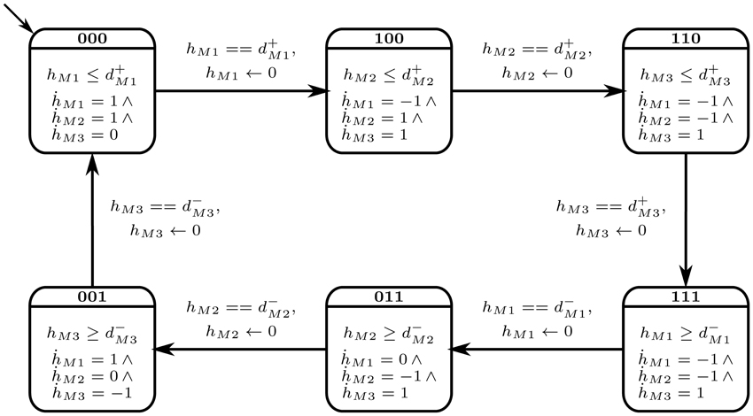
Figure 5. Bio-LHA of Case Study 1: Microbial Population.

FIGURE 6

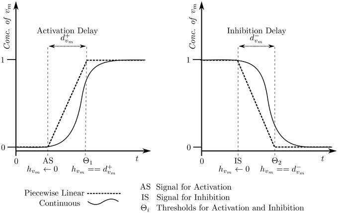
Figure 6. Piecewise affine linear approximation of the continuous evolution of the entity, forming the basis of the hybrid model.

Collectively, the semantics of the of the Bio-LHA are represented as a transition system, adapted from Ahmad et al. (2007) and defined below:

Definition 9. [Semantics of Bio-LHA]. Let γ be a valuation for the parameters P and ν represents the values of clocks in a location. The (𝕋, γ)-semantics of a parametric Bio-LHA 𝔹 is defined as a timed transition system _B = (𝕊, s₀, 𝕋, →) where: (i) 𝕊 = {(ℓ, ν) | ℓ ∈ L and ν ⊨ Inv(ℓ)}, (ii) s₀ is the initial state, and (iii) the relation → ⊆ 𝕊 × 𝕋 × 𝕊 is defined for t ∈ 𝕋 as:

• discrete transitions: (ℓ, ν) $\underrightarrow{0}$ (ℓ′, ν′) iff ∃ (ℓ, g, R, ℓ′) ∈ E such that g(ν) = true, ν′(h) = 0 if h ∈ R and ν′(h) = ν(h) if h ∉ R.

• continuous transitions: For t ∈ 𝕋*, (ℓ, ν) $\underrightarrow{t}$ (ℓ′, ν′) iff ℓ′ = ℓ, ν′(h) = ν(h)+ Dif(ℓ, h) × t, and for every t′ ∈ [0, t], (ν(h) + Dif(ℓ, h) × t′) ⊨ Inv(ℓ), where ⊨ represents satisfaction operator.

In short, the discrete transitions show the transitioning between locations, and is instantaneous. On the other hand, continuous transitions take place within the same location and allows the time to elapse. In Figure 5, the Bio-LHA will remain in the initial location l₀ = (0, 0, 0) as long as the clock variable h_M1 remains less than or equal to d⁺_M1, the activation delay of M1. The rate for that clock is $\dot{h}$_M1 = 1, given below the invariant. Once the clock variable equals d⁺_M1, the continuous transitions can no longer occur. At the same time the guard on the transition h_M1 == d⁺_M1 becomes true and allows a discrete transition from (0, 0, 0) to (1, 0, 0), resetting the clock h_M1 to “0” in the process, provided that the invariant of the next location (1, 0, 0) is not falsified.

The construction of the Bio-LHA further allows the temporal (time based) analysis of the modeled trajectory. The locations themselves represent independent temporal zones, and collectively represent the temporal state space containing discrete transitions between the temporal zones. In this paper, we analyze the invariance kernel of the hybrid models, based on the temporal state space. The invariance kernel represents the entity activation and inhibition timing constraints governing the modeled cyclic oscillating trajectory. Thus, viability is the core of this representation, and can be defined as (adapted from Aubin, 1991; Ahmad et al., 2007; Ahmad, 2009).

Definition 10. [Viability]. Suppose that all trajectories emanating from a particular initial state remain bounded within some constraints, making the trajectories always staying in one sub-domain: namely the viability domain. Such trajectories are called viable trajectories.

The invariance kernel itself is formally defined as (Adapting from Ahmad et al., 2007; Ahmad and Roux, 2010),

Definition 11. [Invariance Kernel]. Let ϕ(t)∈ S ∀ t ≥ 0 be a viable trajectory in the temporal state space S. The largest subset K(S) is the invariance kernel if a trajectory starting at point p is viable in K, ∀p ∈ K.

The algorithm given in our previous study (Ahmad et al., 2007), was utilized to find the invariance kernel for this Bio-LHA. However, the invariance kernel did not converge, indicating that the modeled trajectory may be asymptotic. For such trajectories, the convergence domain analysis (Ahmad and Roux, 2010) provides an over approximation of the delay constraints, within which the trajectory will converge asymptotically. Formally,

Definition 12. [Convergence Domain]. The subset K(S) is called the convergence domain if ∀p ∈ K, the trajectory starting at point p converges in an asymptotic manner.

The convergence domain analysis for Case Study 1 showed 12 conjuncted delay constraints, provided as a table in the Supplementary Materials file. Further analysis of the delay constraints, using a linear constraint solver, allowed us to generate pairwise delay constraint relations between the delay parameters which are given as a matrix in Table 2. The matrix is read row first, column second, from which we can see that the delay relations |d⁻_M3| ≤ d⁺_M1 and d⁺_M3 ≤ |d⁻_M1| are the only significant relations because they represent the constraints which force the system to remain asymptotically within the given cycle. Closer inspection shows that if the constraint |d⁻_M3| ≤ d⁺_M1 is violated, then the microbe M3 will not be inhibited before the activation of microbe M1, understandable as M3 inhibits M1, but it will also nudge the system toward the dominance of M3 over M1 and M2. In terms of ecological balance, this represents how a species can become invasive, displacing other species from the habitat and disrupting other processes dependent on the displaced species. Likewise, if the second constraint d⁺_M3 ≤ |d⁻_M1| is violated, then M2 will be able to inhibit M1 and will in-turn be inhibited before M3 becomes active, diverging into a completely different cycle from the one modeled as the Bio-LHA which can represent the replacement of a particular type of ecological balance with another.

TABLE 2

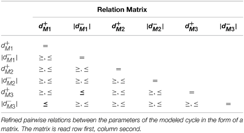
Table 2. The relation matrix of Case Study 1.

2.4. Software

The software SMBioNet (Bernot et al., 2004; Khalis et al., 2009) was used to isolate the logical parameters for both case studies. These parameters, together with the respective regulatory networks, were then constructed in the tool GenoTech (Ahmad et al., 2012), to generate the state graph of the trajectories. Cytoscape (Shannon et al., 2003) was used to conduct centrality analysis of the state graph to isolate particular trajectories. Finally, HyTech (Henzinger et al., 1997) was used to construct the Bio-LHA and analyze the delay constraints of the isolated trajectories.

3. Results

In this section we apply the procedure detailed in the previous section on the slightly larger and more complex Case Study 2, described in Section 1.5.

3.1. Regulatory Network and Logical Parameters

The regulatory network was constructed for Case Study 2, with particular focus on satisfying the given specifications. Its regulatory network, shown in Figure 7, was constructed in the same manner, and shows the positive effects of Sun Shine on the Temperature and Evaporation, the positive effects of the Earth Temperature on Evaporation, the positive effect of Evaporation on Cloud production, the positive effect of Clouds on Water via precipitations, the contribution of the Water source toward Evaporation, as well as the negative effects of Clouds on Sun Shine and themselves (because of precipitation), that of Temperature on Clouds, and of Evaporation on the Water source. For ease in analysis, the names of the entities were shortened to “Temp,” “Sun,” “Evap,” and “Water” for “Temperature,” “Sun Shine,” “Evaporation,” and “Water Source,” respectively. Thus, the formal description of Case Study 2 yields the sets:

• V = {Temp, Sun, Evap, Clouds, Water}, and

• E = {(Sun, Temp), (Sun, Evap), (Temp, Evap), (Temp, Clouds), (Evap, Clouds), (Evap, Water),(Clouds, Clouds), (Clouds, Sun), (Clouds, Water), (Water, Evap)}

FIGURE 7

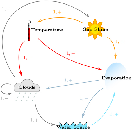
Figure 7. Regulatory network of Case Study 2: Atmospheric system.

After the construction of the regulatory network, the logical parameters were generated using SMBioNet. The observations encoded in CTL checked that from an arbitrary starting state of Sun and Water being available (Temp = 0, Sun = 1, Evap = 0, Clouds = 0, Water = 1), to contain: (i) at least one trajectory where Water is persistently available, and (ii) one cyclic or acyclic trajectory where Water is no longer available after some transitions. Apart from restricting the trivial logical parameters, those parameters for Evap which did not have Water as a resource, and those parameters for Clouds which did not have Evap as resource, were restricted to “0” value in order to reflect the dependence of the entities on their respective resources. A total of 32 sets were generated which satisfied the CTL property, from which a single set given under the “Selected” column of Table 3 was plugged into the Case Study 2 RN.

TABLE 3

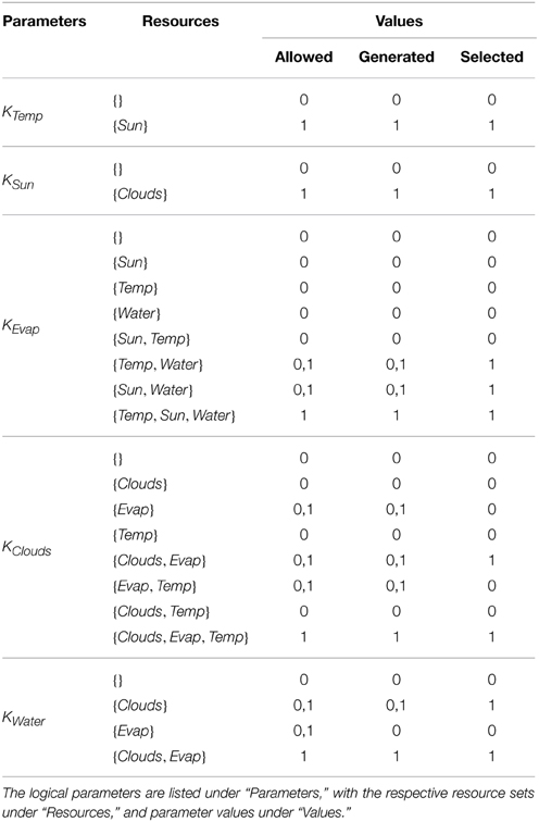
Table 3. Case Study 1: Parameter table.

3.2. State Graphs and Centrality Analysis

After plugging in the logical parameters, the state graphs of Case Study 2 was generated, shown in Figure 8. The state graph contains 566 cyclic trajectories (cycles) and a single deadlock state (1, 1, 0, 0, 0), for the entity order 〈Temp, Sun, Evap, Clouds, Water〉. The deadlock state, in particular, shows a unique configuration where the whole system has turned arid with persistent high temperatures and sun shine.

FIGURE 8

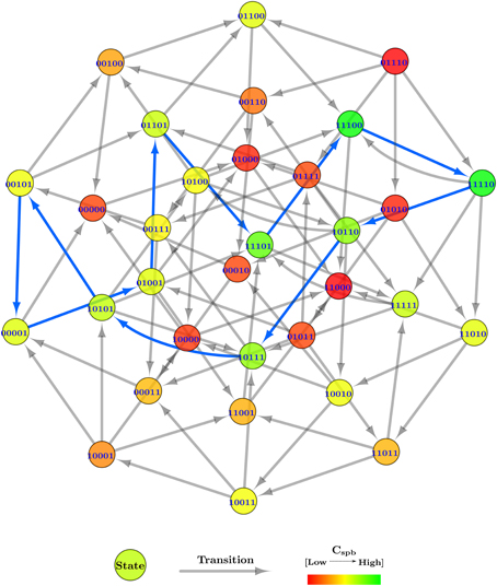
Figure 8. Centrality applied state graph of Case Study 2: Atmospheric system. The cycle selected for hybrid modeling is shown via blue state transitions.

Due to the large number of generated cyclic trajectories, a filtering method was applied in addition to C_spb, by selecting cycles of length 10 only from the total cycles, leaving behind 152 cycles. The reason for the selected length is that it allows all five entities of the system to oscillate between their boolean values, but only once throughout the cycle. To further ease the cycle selection, all 152 cycles were sorted in descending order based on their mean C_spb, instead of using cumulative C_spb for selection as done in Case Study 1 (Section 2.2.2). From the sorted list, the first cycle which had all five entities oscillating was selected, i.e., (0, 1, 0, 0, 1) → (0, 1, 1, 0, 1) → (1, 1, 1, 0, 1) → (1, 1, 1, 0, 0) → (1, 1, 1, 1, 0) → (1, 0, 1, 1, 0) → (1, 0, 1, 1, 1) → (1, 0, 1, 0, 1) → (0, 0, 1, 0, 1) → (0, 0, 0, 0, 1) → (0, 1, 0, 0, 1), having the mean C_spb = 0.145 approximately. The cycle is shown via blue transitions in Figure 8, and starts in the initial state with the sun shining and a water source available, collectively inducing evaporation in the second state. Meanwhile, the temperature also increases as indicated in the third state, while the water source is drained due to persistent evaporation in the fourth state. Afterwards, clouds are formed in the fifth state due to the evaporated water vapors, blocking out the sun in the sixth state, and rejuvenating the water source in the seventh state via precipitation. The clouds disseminate in the eighth state because of the collective effect of precipitation and high temperatures. However, due to persistent blockage of the sun in the previous states, the temperature also goes down in the ninth state, effectively stopping evaporation in the 10th state. Given that the clouds have been disseminating for a while now, the sun begins to shine again, bringing the whole trajectory to its initial state.

3.3. Hybrid Modeling and Delay Constraints

The selected cyclic trajectory was then converted to a Bio-LHA, as shown in Figure 9. The rates for each entity were set based on the immediate successors of the state in the state graph, unlike Case Study 1 where anticipation was used to set the rates. The primary reason is that in biological systems, a small concentration of a source entity can start affecting its target entities, thus initiating their activation or inhibition early (before achieving the threshold). In larger environmental systems, on the other hand, a small concentration of the source entity has negligible effects on its target entities, thus we forgo the concept of anticipation for Case Study 2. Once set, the algorithm cited in Section 2.3 was used to find the invariance kernel of the cycle, converging upon a single set of delay constraints. The seven non-trivial conjuncted constraints are provided in the Supplementary Materials file.

FIGURE 9

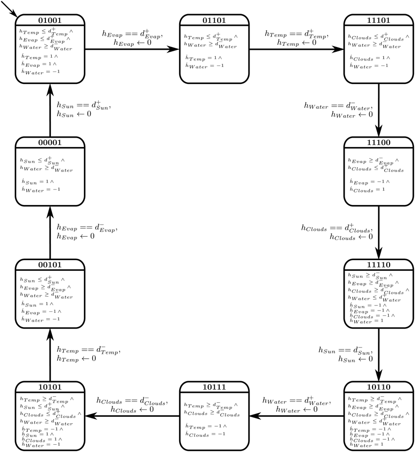
Figure 9. Bio-LHA of Case Study 2: Atmospheric System. To improve readability, only the clock variables with non-zero rates are shown in each location.

The constraints were then fed to the linear constraint solver to generate the pairwise relation matrix given in Table 4, revealing nine significant constraint relations. These significant relations force the trajectory to remain within the cycle, and violation of these relations will diverge the system toward other cyclic or acyclic trajectories. Thus, the violation of the constraint d⁺_Evap ≤ d⁺_Temp will diverge the system toward states where the activation of Temperature occurs before Evaporation, possibly restricting or limiting the production of Clouds due to persistent high temperature. Likewise, the inhibition delay of the Water entity (|d⁻_Water|) strictly takes more duration than activation of Temperature, activation of Sun Shine, and activation of Evaporation. Violation of the first relation will allow the Water Source to be drained before the ultimate activation of Temperature, nudging the trajectory closer to the deadlock state. Then, in the relation d⁺_Water ≤ |d⁻_Clouds|, it is clear that the Water Source should be replenished before the dissemination of the Clouds, the violation of which will also diverge the trajectory toward the deadlock state. Recall that the deadlock state is (1, 1, 0, 0, 0).

TABLE 4

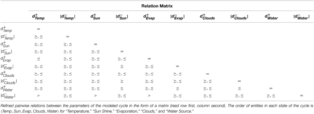
Table 4. The relation matrix of Case Study 2.

4. Discussion

Although the application of Parametric Biological Linear Hybrid Automata is not new (Ahmad et al., 2009, 2012; Aslam et al., 2014; Paracha et al., 2014 to name a few), in this paper we present its application to a new set of problems, namely the modeling of environmental systems. We successfully model two case studies representing different systems from a broad spectrum of mechanisms encompassed by environmental systems, which shows the versatility of the modeling framework toward its applicability. In the first case study, our framework modeled the arbitrary population levels between different microbes in a freshwater pond, showing how hybrid modeling can be used to study different behavioral tendencies of the populations represented by population balance (cyclic trajectories) and overpopulation (deadlocked trajectory), while removing the complexity of dealing with actual population numbers. In the second case study, the modeling framework was applied on a slightly more complex atmospheric system, providing us with the constrained dynamics that the system exhibits in a particular trajectory, while also pinpointing particular constrained relations between parameters which are essential to keep a trajectory stable and non-divergent.

In the analysis of the two case studies, the hybrid framework and application methodology was able to answer all objections pertaining to other methodologies raised in Section 1.2, namely that this methodology (i) presents the complete dynamics of the system in the form of state graphs, (ii) is able to deterministically predict different behaviors via delay constraints, (iii) whilst keeping the complexity of the system manageable. Another possibility is the conversion of the hybrid to a continuous model via Timed Hybrid Petri Nets (David and Alla, 2010) where these delay constraints can be applied using arbitrary numeric values to timed or continuous transitions. The advantage of this conversion is that precise perturbations (disturbances) and what-if scenarios can be constructed to experiment and analyze the system, resulting in added insights of the behavioral dynamics of the system when faced with different stimuli.

That being said, the approach has its limitations, primarily the number of entities being modeled. Although theoretically any number of entities can be modeled, practically the complexity and state space of the system increase exponentially with the number of entities, leading to state space explosion. This limitation puts a major emphasis on effective abstraction of the system in order to preserve the behaviors of the system whilst representing as few entities as possible. Although useful, there are times when a large number of entities need to be represented for different purposes (Hanrahan, 2010), leaving abstraction a bitter-sweet process. In Conclusion, the application of Parametric Biological Linear Hybrid Automata allows the modeling of complex environmental systems for the analysis of behavioral dynamics of these system.

Author Contributions

Study design: ST, JA, OR; Experiments: ST; Analyses: ST, JA; Write-up and review: ST, JA, OR.

Conflict of Interest Statement

The authors declare that the research was conducted in the absence of any commercial or financial relationships that could be construed as a potential conflict of interest.

Acknowledgments

The authors acknowledge the valuable input of the respected reviewers for the improvement of quality of this research article.

Supplementary Material

The Supplementary Material for this article can be found online at: https://www.frontiersin.org/article/10.3389/fenvs.2015.00047

Supplemental Data

A supplementary materials file is provided which contains the SMBioNet and HyTech source codes of both case studies, along with the respective convergence domain and invariance kernel tables.

References

Ahmad, J., and Roux, O. (2010). Invariance kernel of biological regulatory networks. Int. J. Data Mining Bioinformatics 4, 553–570. doi: 10.1504/IJDMB.2010.035900

PubMed Abstract | CrossRef Full Text | Google Scholar

Ahmad, J., Richard, A., Bernot, G., Comet, J.-P., and Roux, O. (2006). “Delays in biological regulatory networks (brn),” in Computational Science ICCS 2006, Vol. 3992 of Lecture Notes in Computer Science eds V. Alexandrov, G. van Albada, P. Sloot, and J. Dongarra (Berlin; Heidelberg: Springer), 887–894.

Ahmad, J., Bernot, G., Comet, J.-P., Lime, D., and Roux, O. (2007). Hybrid modelling and dynamical analysis of gene regulatory networks with delays. Complexus 3, 231–251. doi: 10.1159/000110010

CrossRef Full Text | Google Scholar

Ahmad, J., Roux, O., Bernot, G., and Comet, J.-P. (2008). Analysing formal models of genetic regulatory networks with delays. Int. J. Bioinformatics Res. Appl. 4, 240–262. doi: 10.1504/IJBRA.2008.019573

PubMed Abstract | CrossRef Full Text | Google Scholar

Ahmad, J., Bourdon, J., Eveillard, D., Fromentin, J., Roux, O., and Sinoquet, C. (2009). Temporal constraints of a gene regulatory network: refining a qualitative simulation. Bio Syst. 98, 149–159. doi: 10.1016/j.biosystems.2009.05.002

PubMed Abstract | CrossRef Full Text | Google Scholar

Ahmad, J., Niazi, U., Mansoor, S., Siddique, U., and Bibby, J. (2012). Formal modeling and analysis of the mal-associated biological regulatory network: insight into cerebral malaria. PLoS ONE 7:e33532. doi: 10.1371/journal.pone.0033532

PubMed Abstract | CrossRef Full Text | Google Scholar

Ahmad, J. (2009). Modélisation Hybride et Analyse des Dynamiques des Réseaux de Régulations Biologiques en Tenant Compte des Délais. Ph.D. thesis, Ecole Centrale de Nantes.

Aslam, B., Ahmad, J., Ali, A., Paracha, R., Tareen, S., Niazi, U., et al. (2014). On the modelling and analysis of the regulatory network of dengue virus pathogenesis and clearance. Comput. Biol. Chem. 53, 277–291. doi: 10.1016/j.compbiolchem.2014.10.003

PubMed Abstract | CrossRef Full Text | Google Scholar

Aubin, J. P. (1991). Viability Theory. Cambridge, MA: Birkhauser Boston Inc.

Google Scholar

Berie, H. (2014). Suitability analysis for jatropha curcas production in ethiopia - a spatial modeling approach. Environ. Syst. Res. 3, 25. doi: 10.1186/s40068-014-0025-7

CrossRef Full Text

Bernot, G., Comet, J.-P., Richard, A., and Guespin, J. (2004). Application of formal methods to biological regulatory networks: extending thomas asynchronous logical approach with temporal logic. J. Theor. Biol. 229, 339347. doi: 10.1016/j.jtbi.2004.04.003

PubMed Abstract | CrossRef Full Text | Google Scholar

Casulli, V., and Zanolli, P. (2002). Semi-implicit numerical modeling of nonhydrostatic free-surface flows for environmental problems. Math. Comput. Model. 36, 1131–1149. doi: 10.1016/S0895-7177(02)00264-9

CrossRef Full Text | Google Scholar

Clarke, E. M. Jr., Grumberg, O., and Peled, D. A. (1999). Model Checking. Cambridge, MA: MIT Press.

Google Scholar

Coulthard, T., Lewin, J., and Macklin, M. (2005). Modelling differential catchment response to environmental change. Geomorphology 69, 222–241. doi: 10.1016/j.geomorph.2005.01.008

CrossRef Full Text | Google Scholar

Crooks, A., Castle, C., and Batty, M. (2008). Key challenges in agent-based modelling for geo-spatial simulation. Comput. Environ. Urban Syst. 32, 417–430. doi: 10.1016/j.compenvurbsys.2008.09.004

CrossRef Full Text | Google Scholar

David, R., and Alla, H. (2010). Discrete, Continuous, and Hybrid Petri Nets. Berlin; Heidelberg: Springer.

Google Scholar

Gottschalk, F., Sonderer, T., Scholz, R. W., and Nowack, B. A. (2010). Possibilities and limitations of modeling environmental exposure to engineered nanomaterials by probabilistic material flow analysis. Environ. Toxicol. Chem. 29, 1036–1048. doi: 10.1002/etc.135

PubMed Abstract | CrossRef Full Text | Google Scholar

Hanrahan, G. (2010). Modelling of Pollutants in Complex Environmental Systems. Hertfordshire: ILM Publications.

Google Scholar

Henzinger, T. A., Ho, P.-H., and Wong-Toi, H. (1997). “Hytech: a model checker for hybrid systems,” in Computer Aided Verification, ed O. Grumberg (Heidelberg: Springer), 460–463.

Google Scholar

Juncker, B. H., and Schreiber, F. (2008). Analysis of Biological Networks. Hoboken, NJ: John Wiley & Sons, Inc.

Google Scholar

Kanevski, M., Parkin, R., Pozdnukhov, A., Timonin, V., Maignan, M., Demyanov, V., et al. (2004). Environmental data mining and modeling based on machine learning algorithms and geostatistics. Environ. Model. Softw. 19, 845–855. doi: 10.1016/j.envsoft.2003.03.004

CrossRef Full Text | Google Scholar

Kauffman, S. (1969). Metabolic stability and epigenesis in randomly constructed genetic nets. J. Theor. Biol. 22, 437–467. doi: 10.1016/0022-5193(69)90015-0

PubMed Abstract | CrossRef Full Text | Google Scholar

Khalis, Z., Comet, J.-P., Richard, A., and Bernot, G. (2009). The SMBioNet method for discovering models of gene regulatory networks. Genes Genomes Genomics 3, 15–22.

Google Scholar

Paracha, R., Ahmad, J., Ali, A., Hussain, R., Niazi, U., Tareen, S., et al. (2014). Formal modelling of toll like receptor 4 and jak/stat signalling pathways: insight into the roles of socs-1, interferon-β and proinflammatory cytokines in sepsis. PLoS ONE 9:e108466. doi: 10.1371/journal.pone.0108466

PubMed Abstract | CrossRef Full Text | Google Scholar

Refsgaard, J. C., van der Sluijs, J. P., Hjberg, A. L., and Vanrolleghem, P. A. (2007). Uncertainty in the environmental modelling process a framework and guidance. Environ. Model. Softw. 22, 1543–1556. doi: 10.1016/j.envsoft.2007.02.004

CrossRef Full Text | Google Scholar

Sengupta, R. R., and Bennett, D. A. (2003). Agent-based modelling environment for spatial decision support. Int. J. Geogr. Inf. Sci. 17, 157–180. doi: 10.1080/713811747

PubMed Abstract | CrossRef Full Text | Google Scholar

Seppelt, R. (2007). Computer-Based Environmental Management. Wiley-VCH Verlag GmbH & Co. KGaA.

Google Scholar

Shannon, P., Markiel, A., Ozier, O., Baliga, N., Wang, J., Ramage, D., et al. (2003). Cytoscape: a software environment for integrated models of biomolecular interaction networks. Genome Res. 13, 2498–2504. doi: 10.1101/gr.1239303

PubMed Abstract | CrossRef Full Text | Google Scholar

Somlydy, L. (1982). Modelling a complex environmental system: the lake balaton study. Math. Model. 3, 481–502. doi: 10.1016/0270-0255(82)90044-6

CrossRef Full Text | Google Scholar

Sun, T. Y., Gottschalk, F., Hungerbhler, K., and Nowack, B. (2014). Comprehensive probabilistic modelling of environmental emissions of engineered nanomaterials. Environ. Pollut. 185, 69–76. doi: 10.1016/j.envpol.2013.10.004

PubMed Abstract | CrossRef Full Text | Google Scholar

Ttrai, I., Mtys, K., Korponai, J., Paulovits, G., and Pomogyi, P. (2000). The role of the kis-balaton water protection system in the control of water quality of lake balaton. Ecol. Eng. 16, 73–78. doi: 10.1016/S0925-8574(00)00091-4

PubMed Abstract | CrossRef Full Text | Google Scholar

Thomas, R. (1979). Kinetic logic: a boolean approach to the analysis of complex regulatory systems. Lect. Notes Biomath. 29, 507.

PubMed Abstract | Google Scholar

Thomas, R. (1998). Laws for the dynamics of regulatory networks. Int. J. Dev. Biol. 42, 479–485.

PubMed Abstract | Google Scholar

Thomas, R., and d'Ari, R. (1990). Biological Feedback. Boca Raton, FL: CRC Press.

Google Scholar

Thomas, R., Thieffry, D., and Kaufman, M. (1995). Dynamical behaviour of biological regulatory networks-i. biological role of feedback loops and practical use of the concept of the loop-characteristic state. Bull. Math. Biol. 57, 247–276.

PubMed Abstract | Google Scholar

Thomas, R. (1978). Logical analysis of systems comprising feedback loops. J. Theor. Biol. 73, 631–656.

PubMed Abstract | Google Scholar

Uusitalo, L. (2007). Advantages and challenges of bayesian networks in environmental modelling. Ecol. Model. 203, 312–318. doi: 10.1016/j.ecolmodel.2006.11.033

CrossRef Full Text | Google Scholar

Wiley, E., McNyset, K. M., Peterson, A. T., Robins, C. R., and Stewart, A. M. (2003). Niche modeling and geographic range predictions in the marine environment using a machine-learning algorithm. Oceanography 16, 120–127. doi: 10.5670/oceanog.2003.42

CrossRef Full Text | Google Scholar

Appendix

TABLE A1

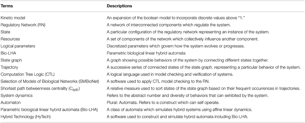
Table A1. Glossary of technical terms.