Reactivity and stability of large ecosystems

1. Introduction

The relationship between complexity and stability of ecological communities has been an important driver of theoretical ecology (e.g., Yodzis, 1981; Pimm, 1984; McCann, 2000; May, 2001; Martinez et al., 2005). This interest was sparked by the work of Robert May, who in 1972 showed that large random communities are inevitably unstable (May, 1972). In unstable communities, even infinitesimal perturbations would drive the system away from steady-state and potentially lead to the loss of species. Since May's work, ecologists have been trying to find mechanisms that can stabilize natural ecosystems and support the staggering biodiversity observed empirically (e.g., McNaughton, 1978; Yodzis, 1981; McCann et al., 1998; Emmerson and Yearsley, 2004). Recently, we extended May's results on randomly assembled systems to communities with certain interaction types, such as predator-prey (i.e., food webs), mutualistic and competitive communities (Allesina and Tang, 2012). Starting—as May did—directly from the “community matrix” (Levins, 1968) describing the effects of species on each other around an equilibrium point, we derived stability criteria for large, complex ecosystems, and showed that a large number of species can coexist at a locally stable equilibrium if predator-prey interactions are preponderant.

Clearly, stable ecosystems are more likely to persist in time than unstable ones. However, stability only expresses the long-term response to small perturbations. Transient dynamics, observed in many ecological models and communities (Neubert and Caswell, 1997; Chen and Cohen, 2001; Hastings, 2004; Rozdilsky et al., 2004) as well as in other dynamical systems (Farrell and Ioannou, 1996; Schmid, 2007), can be remarkably different from the long-term dynamics and thus also play an important role for the persistence of such systems. In fact, some perturbations of a stable equilibrium might be initially amplified before decaying. In ecology, stable equilibria with this property are called “reactive” (Neubert and Caswell, 1997). Such initial amplifications of the perturbations drive the system even further from the equilibrium state, and thus increase the risk of stochastic extinction. The concept of reactivity was first introduced to ecology by Neubert and Caswell (1997) and it complements that of stability: stability describes the long-term, asymptotic behavior in response to perturbations, whereas reactivity describes the immediate response for stable equilibria (Farrell and Ioannou, 1996). Reactivity quantifies the maximum instantaneous amplification rate of infinitesimal perturbations. As such, in highly reactive systems, small perturbations can be initially greatly amplified before decaying, with potentially important consequences for stochastic extinctions. Reactivity has been studied in many ecological contexts, including food web models (Chen and Cohen, 2001), structured population models (Caswell and Neubert, 2005), and infectious diseases (Hosack et al., 2008).

Here, we study the relationship between stability and reactivity in randomly assembled ecosystems. After establishing a criterion for reactivity in large ecosystems, we show that the same quantities determine both stability and reactivity: both criteria can be written as inequalities involving the number of species (S), expectations of the intra- and inter-specific interaction strengths (E and −d, respectively), variance of inter-specific interactions (V), and correlation between pairs of interactions (ρ).

By comparing the criteria for stability and reactivity, we find that for fixed S, V, E, and ρ, making an equilibrium non-reactive and stable requires stronger intra-specific interaction than that necessary to achieve stability. Numerical simulations confirm our findings: starting from an unstable equilibrium, if we gradually increase the mean strengths of intra-specific interactions, the equilibrium of the system first becomes reactively stable, and then becomes non-reactively stable.

This implies that reactive stability is an intermediate phase separating non-reactive stability and instability. As such, reactivity could be exploited as an early-warning signal for catastrophic regime shifts in ecosystems, an area of ecology that is experiencing rapid growth (May, 1977; Wissel, 1984; Scheffer et al., 2001, 2009, 2012).

2. Material and Methods

2.1. Stability Analysis

Consider an ecological community composed of S species, whose population densities at any time t are denoted as a vector Y(t) of length S. Species dynamics are typically modeled by a system of non-linear autonomous ordinary differential equations:

$\begin{array}{cc}\frac{dY(t)}{dt}=f(Y)& \left(1\right)\end{array}$

where f = [f₁, f₂, …, f_S]^T is a set of functions describing the dynamics of the S species. A feasible equilibrium point of system (1) is a non-negative vector Y* = [Y*₁, Y*₂, …, Y*_S]^T such that:

$\begin{array}{cc}f(Y^{\ast })=0& \left(2\right)\end{array}$

The evolution of a small perturbation y₀ = ΔY(0) applied to the equilibrium Y* can be approximated by the linear equation:

$\begin{array}{cc}\frac{d(\Delta Y(t))}{dt}=M·\Delta Y& \left(3\right)\end{array}$

where M is the so-called “community matrix” (Levins, 1968; May, 1972, 2001): the Jacobian matrix evaluated at the equilibrium, i.e.,

$\begin{array}{cc}{M}_{ij}={\frac{\partial f_i}{\partial Y_j}|}_{Y=Y^{\ast }}& \left(4\right)\end{array}$

An equilibrium is called “(locally asymptotic) stable” if any infinitesimal perturbation decays to zero eventually: for any ΔY(0) sufficiently small, we have lim_{t → ∞}ΔY(t) = 0. Moreover, if all eigenvalues of M, denoted by λ^M_i, i = 1, 2, …, S, have negative real parts, the equilibrium point is stable (May, 1972, 2001). Here we always order the eigenvalues of M such that ℜ(λ^M₁) ≤ ℜ(λ^M₂) ≤ ··· ≤ ℜ(λ^M_S). Thus if ℜ(λ^M_S) < 0, the equilibrium is stable.

2.2. Reactivity Analysis

The stability of an equilibrium defines the long-term response to small perturbations. However, the real parts of M's eigenvalues do not provide information on the instantaneous response to perturbations. Among stable equilibria, the instantaneous dynamics can differ dramatically, even if all perturbations will eventually die out.

Neubert and Caswell (1997) firstly introduced to ecology the concept of reactivity, which quantifies the maximum amplification rate of perturbations. For reactive equilibria, some perturbations will immediately grow in magnitude before eventually decaying. Conversely, if all small perturbations decay immediately, such equilibria are non-reactive. As such, reactivity is defined as the maximal initial amplification rate, which can be calculated from:

$\begin{array}{cc}\begin{array}{l}\text{Reactivity }=\underset{{}_{||y_0||\ne 0}}{\max }\left[{\left\{\frac{1}{||\Delta Y(t)||}\frac{d||\Delta Y(t)||}{dt}\right\}|}_{t=0}\right]\\ =\max \left({\lambda }_i^H\right)={\lambda }_S^H\end{array}& \left(5\right)\end{array}$

where ||·|| is the norm operator. Neubert and Caswell also showed that the maximum initial amplification rate is simply λ^H_S, the largest eigenvalue of H, where H is the symmetric part of the community matrix M, defined as $H=\frac{M+M^T}{2}$, where M^T is the transpose of M. Note that H is symmetric and therefore all its eigenvalues are real. An equilibrium is reactive if λ^H_S > 0 (i.e., positive instantaneous amplification rate) and non-reactive if λ^H_S < 0 (i.e., negative instantaneous amplification rate) (Neubert and Caswell, 1997). For any matrix M, we have that λ^H_S ≥ ℜ(λ^M_S) (Snyder, 2010): the largest real part for the eigenvalues of M is bounded from above by the largest eigenvalue of the symmetric matrix $H=\frac{M+M^T}{2}$, and the largest imaginary part is bounded from above by the largest eigenvalue of the symmetric matrix $H^{\prime }=\frac{M-M^T}{2}$ (Wolkowicz and Styan, 1980). As such, unstable equilibria (ℜ(λ^M_S) > 0) are certainly reactive (λ^H_S > 0), whereas stable equilibria (ℜ(λ^M_S) < 0) can be either reactive or non-reactive.

2.3. Building Community Matrices

As when studying stability (Tang et al., in press), the diagonal entries of M are assumed to have a negative expectation 𝔼 (M_ii) < 0; and we denote 𝔼 (M_ii) = −d for some positive number d. The diagonal entries are sampled independently from a normal distribution with mean −d and finite variance σ²_d. The off-diagonal entries of M are sampled as independent pairs according to a bivariate distribution of (X₁, X₂) in the following way: (1) with probability C/2, (M_ij, M_ji)_{i > j} is sampled from the distribution of (X₁, X₂); (2) with probability C/2, (M_ij, M_ji)_{i l > j} is sampled from the distribution of (X₂, X₁); (3) with probability (1 − C), (M_ij, M_ji)_{i > j} = (0, 0). The symmetric part of M is computed from the definition $H=\frac{M+M^T}{2}$. Note that M constructed in this way can describe different types of communities when we vary the underlying bivariate distribution. For example, when (X₁, X₂) is chosen to follow a bivariate mean-zero Gaussian distribution, with two independent components, M can represent the collection of randomly-assembled communities studied by May (1972). If the distribution is defined such that the two components X₁ and X₂ always have opposite signs, then M can represent a food web, containing only consumer-resource interactions, as in Allesina and Tang (2012).

2.4. Derivation of the Reactivity Criteria

For a random matrix M whose entries are independently sampled from a statistical distribution, five quantities are essential for determining the largest real part of its eigenvalues: (1) S, the dimension of M, which equals the number of species in the network, (2) E, the expectation of the off-diagonal entries, describing inter-specific interaction strengths, (3) −d, the expectation of the diagonal entries, describing intra-specific interaction strengths, (4) V, the variance of the off-diagonal entries, and (5) ρ, the pairwise interaction correlation:

$\begin{array}{l}E=E^M=𝔼{(M_{ij})}_{i\ne j},d=d^M=-𝔼(M_{ii})>0,\\ V=V^M=\text{Var}{(M_{ij})}_{i\ne j}\ge 0\\ \rho ={\rho }^M=\frac{E_2-E^2}{V}\in [-1,1],\text{ where }\\ E_2=E_2^M=𝔼{(M_{ij}{M}_{ji})}_{i\ne j}\end{array}$

In Allesina and Tang (2012) and Tang et al. (in press), we showed that there is always one eigenvalue of M (denoted by λ^M_R) whose real part is close to the expected row sum of M:

$\begin{array}{cc}\Re \left({\lambda }_R^M\right)\approx (S-1)E-d& \left(6\right)\end{array}$

When S is sufficiently large, the other (S − 1) eigenvalues of M are approximately uniformly distributed on an ellipse centered at (−E −d, 0), whose horizontal and vertical axes are about 2$\sqrt{SV}$(1 + p) and 2$\sqrt{SV}$(1 − p), respectively. Thus the rightmost one of these (S − 1) eigenvalues (denoted by ℜ(λ^M_EL)) can be estimated using the “center” plus the semi-length of the horizontal axis:

$\begin{array}{cc}\Re \left({\lambda }_{EL}^M\right)\approx -E-d+\sqrt{SV}(1+\rho )& \left(7\right)\end{array}$

Depending on the sign and the magnitude of ℜ(λ^M_R), stability may be determined by either ℜ(λ^M_R) or ℜ(λ^M_EL), i.e., the largest real part for all eigenvalues of M is just the larger one of these two eigenvalues:

$\Re \left({\lambda }_S^M\right)=\max \left\{\Re \left({\lambda }_R^M\right),\Re \left({\lambda }_{EL}^M\right)\right\}$

When E > 0, ℜ(λ^M_R) grows linearly in S whereas ℜ(λ^M_EL) grows only sub-linearly, so if S is sufficiently large, for example, $S\gg \frac{V{(1+\rho )}^2}{E^2}$, we have:

$(S-1)E-d>\sqrt{SV}(1+\rho )-E-d$

In this case, λ^M_R lies on the right of the ellipse formed by the other (S − 1) eigenvalues, and the largest real part of the eigenvalues of M is thus ℜ(λ^M_R), i.e., for sufficiently large S,

$\Re \left({\lambda }_S^M\right)=\Re \left({\lambda }_R^M\right)\approx (S-1)E-d$

When E ≤ 0, we always have

$(S-1)E-d<\sqrt{SV}(1+\rho )-E-d,$

which means λ^M_R lies on the left of the ellipse. Hence the rightmost eigenvalue of M is λ^M_EL. In this case, for sufficiently large S, we have

$\Re \left({\lambda }_S^M\right)=\Re \left({\lambda }_{EL}^M\right)\approx \sqrt{SV}(1+\rho )-E-d$

A random, symmetric matrix, such as H, is a special case of general random matrices. As such, we may use the same approach to estimate the largest eigenvalue of H. We thus compute the corresponding statistical quantities for H, namely,

$\begin{array}{l}{E}^H=𝔼{(H_{ij})}_{i\ne j},d^H=-𝔼(H_{ii})>0,\\ V^H=\text{Var}{(H_{ij})}_{i\ne j}\ge 0,\\ {\rho }^H=\frac{E_2^H-{\left(E^H\right)}^2}{V^H}\in [-1,1],\text{ where }{E}_2^H=𝔼{(H_{ij}{H}_{ji})}_{i\ne j}\end{array}$

In particular, we would like to express these five quantities in terms of the statistics of M. First of all, the expectations of the diagonal and off-diagonal entries do not change by taking the symmetric part of M, because

$\begin{array}{l}{E}^H=𝔼{(H_{ij})}_{i\ne j}=𝔼{\left(\frac{M_{ij}+M_{ji}}{2}\right)}_{i\ne j}\\ =\frac{𝔼{(M_{ij})}_{i\ne j}+𝔼{(M_{ji})}_{i\ne j}}{2}=E\\ d^H=-𝔼(H_{ii})=-𝔼(M_{ii})=d\end{array}$

However, the variance, the expectation of the products of pairwise interactions, and the pairwise correlation do differ in M and H. These quantities for H can be computed according to the relationship between M and H:

$\begin{array}{l}{V}^H=\text{Var}{(H_{ij})}_{i\ne j}=\text{Var}{\left(\frac{M_{ij}+M_{ji}}{2}\right)}_{i\ne j}\\ =\frac{V}{2}+\frac{\text{Cov}{(M_{ij},M_{ji})}_{i\ne j}}{2}\\ =\frac{V}{2}+\frac{E_2-E^2}{2}=\frac{V}{2}\left(1+\frac{E_2-E^2}{V}\right)=\frac{V}{2}(1+\rho )\\ E_2^H=𝔼{(H_{ij}{H}_{ji})}_{i\ne j}=𝔼{\left(H_{ij}^2\right)}_{i\ne j}=\text{Var}{(H_{ij})}_{i\ne j}+{𝔼}^2(H_{ij})\\ =V^H+{\left(E^H\right)}^2\\ {\rho }^H=\frac{E_2^H-{\left(E^H\right)}^2}{V^H}=\frac{V^H}{V^H}=1\end{array}$

Similar to the case of stability, two eigenvalues of H are essential in determining the reactivity of the underlying equilibrium, one corresponding to the expected row sum (denoted by λ^H_R), and the other one corresponding to the largest one among the other (S − 1) eigenvalues forming an “ellipse.” In the case of symmetric matrices, since ρ^H = 1, the vertical axis of the ellipse is zero:

$2\sqrt{S{V}^H}\left(1-{\rho }^H\right)=0$

This means the ellipse actually degenerates to a line segment on the real axis. The density of the eigenvalues of a random symmetric matrix is described by Wigner's semicircle law (Wigner, 1958), so we denote the largest eigenvalue among the S − 1 eigenvalues (excluding λ^H_R) by λ^H_SC, where “_SC” stands for “semicircle.” Similarly to the computation of ℜ(λ^M_R) and ℜ(λ^M_EL), λ^H_R and λ^H_SC can be computed as follows:

$\begin{array}{l}{\lambda }_R^H\approx (S-1)E^H-d^H=(S-1)E-d\\ {\lambda }_{SC}^H\approx \sqrt{S{V}^H}\left(1+{\rho }^H\right)-E^H-d^H=\sqrt{2SV(1+\rho )}-E-d\end{array}$

These equations are analogous to those determining stability (Equations 6, 7): the only difference is that instead of using E, V, and ρ for matrix M, we take the corresponding values for matrix H.

Again, the largest eigenvalue of H is the larger one of λ^H_R and λ^H_SC:

${\lambda }_S^H=\max \left({\lambda }_R^H,{\lambda }_{SC}^H\right)$

If E > 0, for sufficiently large S, namely $S\gg \frac{2V(1+\rho )}{E^2}$, we have λ^H_R > λ^H_SC

$\begin{array}{cc}{\lambda }_S^H={\lambda }_R^H\approx (S-1)E-d& \left(8\right)\end{array}$

whereas if E ≤ 0, the largest eigenvalue of H is λ^H_SC and thus

$\begin{array}{cc}{\lambda }_S^H={\lambda }_{SC}^H\approx \sqrt{2SV(1+\rho )}-E-d& \left(9\right)\end{array}$

2.5. Simulating the Phase Transitions for Stability and Reactivity

We use numerical simulations to verify the derivation of the reactivity criteria. We choose S = 250, C = 0.2, and standard normal distribution (0, 1) for the marginal distributions of X₁ and X₂. We consider three different cases of the joint distribution (X₁, X₂). The first case is called the Random case, where X₁ and X₂ follow independent (0, 1) distributions and (M_ij, M_ji)_{i > j} can be (+, −), (−, +), (+, +), or (−, −). In this case, we have E = 0, V = C, and ρ = 0. The second case is called the Predator-Prey case, where we constrain the two entries in each non-zero pair (M_ij, M_ji)_{i > j} to have different signs, either (+, −) or (−, +), and this also gives E = 0, V = C, but a negative pairwise correlation $\rho =\frac{E_2}{V}=\frac{-C𝔼\left|X_1\right|𝔼\left|X_2\right|}{C}=-\frac{2}{\pi }<0$. The last case is the Mixture of mutualism and competition case (or “Mixture” case for short), where each non-zero pair (M_ij, M_ji)_{i < j} contains two entries of the same sign, either (+, +) or (−, −). In the Mixture case, we still have E = 0, V = C, but a positive pairwise correlation $\rho =\frac{E_2}{V}=\frac{C𝔼\left|X_1\right|𝔼\left|X_2\right|}{C}=\frac{2}{\pi }>0$. The joint distributions of (X₁, X₂) for the three cases are illustrated in Figure 1. To simulate the phase transition for stability and reactivity, we increase d from 0 to 15 (i.e., 𝔼 (M_ii) is between 0 and −15), for three levels of the variances of the diagonal entries σ²_d = 0, 0.5² and 1². For each combination of d and σ_d, we construct 1000 community matrices for each of the three cases, and for each matrix, we check stability and reactivity and estimate the probabilities of stability and reactivity, respectively.

FIGURE 1

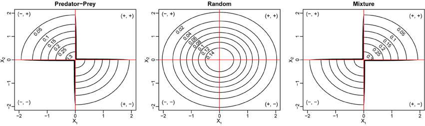
Figure 1. Joint density contour for the bivariate distribution of (X₁, X₂) for three different types of ecological networks. In all three cases, the marginal distributions for both X₁ and X₂ are standard normal distributions.

3. Results

3.1. Stability and Reactivity Criteria

Similar to the derivation for the stability criterion, in which the goal is to estimate the largest real part of the eigenvalues of M, the derivation of the reactivity criterion relies on estimating the largest eigenvalue of H when S is sufficiently large. The reactivity criteria are summarized and compared to their stability counterparts in Table 1. We see that the five quantities affect the largest eigenvalue of H in the same direction as they affect the largest real part of the eigenvalues of M: if changing one quantity while the others are held constant increases (or reduces) ℜ(λ^M_S), such change also increases (or reduces) λ^H_S.

TABLE 1

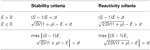
Table 1. Stability and Reactivity Criteria for sufficiently large ecological communities.

If E > 0, for sufficiently large S, ℜ(λ^M_S) and λ^H_S are both of the order (S − 1)E − d, implying that the critical point defining the stability-instability boundary (i.e., when ℜ(λ^M_S) = 0) is asymptotically the same as that for the non-reactivity-reactivity boundary (i.e., when λ^H_S = 0). If E ≤ 0 and S is sufficiently large, ℜ(λ^M_S) and λ^H_S are approximately $\sqrt{SV}$(1 + ρ) − E − d and $\sqrt{2SV(1+\rho )}$ − E − d, respectively. Note that, in this case, since −1 ≤ ρ ≤ 1, we have

$\begin{array}{l}\Re \left({\lambda }_S^M\right)-{\lambda }_S^H\approx \sqrt{SV}(1+\rho )-\sqrt{2SV(1+\rho )}\\ =\sqrt{SV(1+\rho )}\left[\sqrt{1+\rho }-\sqrt{2}\right]\le 0\end{array}$

which yields ℜ(λ^M_S) ≤ λ^H_S. It means we necessarily have ℜ(λ^M_S) < 0 (“stable”) whenever λ^H_S < 0 (“non-reactive”). Our estimate for ℜ(λ^M_S) and λ^M_S are consistent with the fact that a non-reactive equilibrium is always stable (Snyder, 2010).

The assumption of large S is important in determining the rightmost eigenvalue when E > 0. Similar to the study of stability, the reason here is that although λ^H_R grows linearly in S and is eventually larger than λ^H_SC, which grows only sub-linearly, if E is small and S is not sufficiently large, we may still have λ^H_R < λ^H_SC and thus the largest eigenvalue of H is then λ^H_SC instead of λ^H_R. In practice, for a system of a given size S and mean interaction strength E, we need to consider the estimates for both eigenvalues, λ^H_R and λ^H_SC. Similar to the stability criteria derived in Tang et al. (in press), we thus combine the criteria for both E > 0 and E ≤ 0 cases and state the criteria in terms of the maximum of λ^H_R and λ^H_SC (Table 1, row 3).

Note that the expressions for ℜ(λ^M_S) and λ^H_S obtained above are the estimates for their average values. In other words, for fixed S, C, d, and the underlying bivariate distribution (X₁, X₂) (which determines E, E₂, V, and ρ), if one constructs random community matrices M repeatedly, Equations (6–9) provide estimates for the average positions of ℜ(λ^M_S) and λ^H_S among all constructions. For one single realization of M and H, the actual values of ℜ(λ^M_S) and λ^H_S will deviate from their mean estimates due to the randomness. Furthermore, the variations of ℜ(λ^M_S) and λ^H_S around their means decrease with the size of the network: when S is larger, the estimates given in Equations (6–9) are more accurate. Finally, if S ≫ 1 and E is small compared to $\sqrt{SV}$(1 + ρ), we may simplify the expressions in Table 1 accounting for these facts (1) S − 1 ≈ S, (2) $\sqrt{SV}$(1 + ρ) − E ≈ $\sqrt{SV}$(1 + ρ), and (3) $\sqrt{2SV(1+\rho )}$ − E ≈ $\sqrt{2SV(1+\rho )}$.

3.2. The Relation between Stability and Reactivity

From Table 1, we see that the inequalities define the boundary conditions for stability and reactivity. Intuitively, since non-reactive equilibria are necessarily stable but not vice versa, we may think non-reactivity as a stronger form of stability in the sense that all infinitesimal perturbations not only decrease to zero eventually, but also do so immediately.

For fixed S, V, E, and ρ, the negative mean intra-specific interaction d may be viewed as an internal source to stabilize the equilibrium. If d = 0, implying that the eigenvalues of M are centered at zero, we always have unstable and hence reactive equilibrium. When we increase d, which is equivalent to moving the center of the eigenvalues to the left, it is possible to achieve stability and non-reactivity. We denote by d_crit,1 and d_{crit, 2} the minimum (i.e., critical) average strengths of intra-specific interactions needed to achieve stability and non-reactivity, respectively. When E > 0 and S is sufficiently large so that ℜ(λ^M_R) and λ^H_R determine stability and reactivity, respectively, the minimum d required to stabilize or make the equilibrium non-reactive is d_crit,1 = d_crit,2 = (S − 1)E. However, in real ecological networks, the case E < 0 is more common (Tang et al., in press), especially when consumer-resource interactions are preponderant. This is because the positive effects of resources on consumers are usually smaller in magnitude than the negative effects of consumers on resources due to imperfect conversion efficiency. Moreover, adding a higher proportion of competitive interactions compared to mutualistic interaction can make the mean interaction strength even more negative. For this case, the minimum average strength of intra-specific interaction required to stabilize the equilibrium is d_{crit, 1} = $\sqrt{SV}$(1 + ρ) − E, whereas to make the equilibrium non-reactive we need average strength of inter-specific interaction being at least d_{crit, 2} = $\sqrt{2SV(1+\rho )}$ − E, greater than d_crit,1.

Our criteria are quite accurate even for communities of moderate sizes (Figure 2), as confirmed by numerical simulations. In our simulations, when we increase the mean intra-specific interaction strength d, we observe two sequential phase transitions as d passes through the two critical points. First, near d = d_crit,1, the probability of stability rapidly increases from 0 to 1, marking the first phase transition from instability to stability (Figure 2, upward triangles). After that, as d continues to increase, the probability of reactivity rapidly drops from 1 to 0 near d = d_crit,2, marking the second phase transition from reactivity to non-reactivity (Figure 2, downward triangles). As S becomes larger, the behavior for the eigenvalues of M and H will be closer and closer to that estimated according to random matrix theory, and, consequently, the ℜ(λ^M_S) and λ^H_S will be closer and closer to their mean positions (Tang et al., in press). These phase transitions will be sharper for larger S, and the behaviors of the transitions will be more like sudden jumps occurring at d_crit,1 and d_crit,2, respectively. The critical points predicted using our criteria, i.e., d_crit,1 and d_crit,2, are marked by the dashed vertical lines in each case in Figure 2. Conversely, if we start with a non-reactively stable network and gradually push it toward the unstable region, for example, by reducing the mean strength of the intra-specific interactions, the network will first become reactively stable and then unstable. This makes intuitively sense, since if all small perturbations would decay immediately (i.e., non-reactive, stable), then any small perturbation is equivalent to a smaller perturbation in a slightly different direction, which will also decay immediately. Therefore, if a network has a non-reactive, stable equilibrium, it has to first cross the “reactively stable” phase before reaching the unstable phase, assuming its state is changing continuously. Thus, if reactivity were to be detectable in empirical data, it would be an excellent candidate for an early-warning signal for the approach of a bifurcation.

FIGURE 2

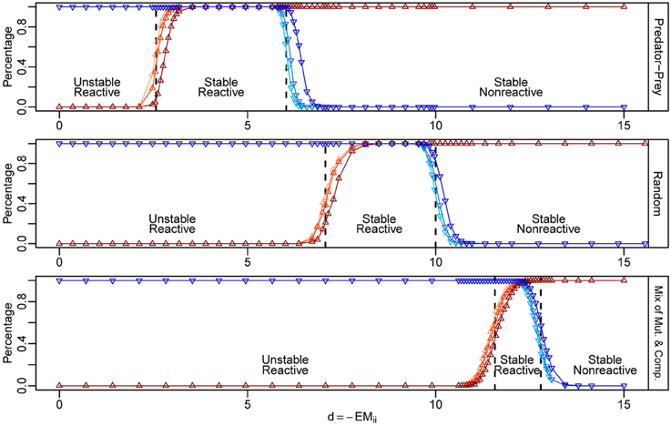
Figure 2. Numerical simulations for the phase transitions of stability and reactivity in three types of ecological networks. The y-axis represents the probability of stability (red) and reactivity (blue) computed from 1000 random community matrices for each case. We built matrices choosing the joint density of (X₁, X₂) as shown in Figure 1. For each type of matrix, we fixed S = 250, C = 0.2, and E = 0. The critical points (d_{crit, 1}, d_{crit, 2}) for the stability-instability and reactivity–non-reactivity transitions are marked by vertical dashed lines. The three regions from left to right correspond to the ranges of d in which the equilibria are unstable, reactively stable, and non-reactively stable. We varied d from 0 to 15, with finer sampling in the regions around the expected phase transition (x-axis). The standard deviation of the intra-specific interaction strengths, σ_d, was set to 0, 0.5, and 1, shown as different shaded curves in each plot, from the lightest to the darkest.

3.3. Stability, Reactivity, and Pairwise Correlation

From the inequalities in Table 1, we see that negative pairwise correlation is beneficial for both stability and non-reactivity. Given the potential of reactivity for signaling the approach of a bifurcation, it is important to know how “early” reactivity can warn us when the system is approaching the unstable state. This is actually measured by the distance between the phase transitions for reactivity and stability, i.e., the absolute difference δ = λ^H_S − ℜ(λ^M_S). When E > 0 and S is sufficiently large, ℜ(λ_S) ≈ λ^H_S and reactivity is asymptotically equivalent to instability. In other cases, either E ≤ 0 or E > 0 but S is not large enough so that we have ℜ(λ^M_S) ≈ $\sqrt{SV}$(1 + ρ) − E − d and λ^H_S ≈ $\sqrt{2SV(1+\rho )}$ − E − d, the difference is

$\delta ={\lambda }_S^H-\Re \left({\lambda }_S^M\right)=\sqrt{SV(1+\rho )}\left(\sqrt{2}-\sqrt{1+\rho }\right)$

depending on S, V, and ρ only. Here, we can see that the absolute distance δ changes monotonically with S and V, indicating that a higher biodiversity results in a larger distance between the two phase transitions. However, δ does not change monotonically with ρ. Computing the first derivative of δ with respect to ρ and equating it to zero, we get:

${\frac{\partial \delta }{\partial \rho }|}_{\rho ={\rho }^{\ast }}=\sqrt{SV}\left(\frac{\sqrt{2}}{2\sqrt{1+{\rho }^{\ast }}}-1\right)=0\Rightarrow {\rho }^{\ast }=-\frac{1}{2}$

The second derivative at ρ* is negative, which implies δ reaches its maximum when $\rho =-\frac{1}{2}$. Thus, for fixed S and V, the distance from the non-reactivity-reactivity phase transition to the stability-instability is large when the interactions between pairs of species maintain a moderate negative correlation (Figure 3).

FIGURE 3

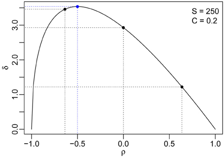
Figure 3. The distance between the two phase transitions (δ) as a function of the pairwise interaction correlation ρ for S = 250 and C = 0.2. The maximum distance and the corresponding pairwise correlation are indicated using blue dashed lines, and the correlations for the three numerical simulations in Figure 2 are marked by black dashed lines.

4. Discussion

The stability and reactivity criteria are derived for ecological networks with random (i.e., Erdős-Rényi) structure. Thus, they cannot directly predict the stability and reactivity of empirical systems, which display markedly non-random structure. However, they can be used as null models to establish an expectation for the ensemble of matrices whose coefficients are distributed as in the empirical system, but have random structure. This effectively serves as a way to determine the influence of network structure on stability and reactivity.

The criteria are to be interpreted in a probabilistic sense. We have shown that the stability and reactivity criteria are derived based on the estimates of the average positions of ℜ(λ^M_S) and λ^H_S, obtained repeatedly constructing the community matrix M and its symmetric part H using the same parameters, underlying bivariate distribution, and algorithm. For each realization of M and H, ℜ(λ^M_S) and λ^H_S are around their predicted positions, with smaller variation when S is larger. Therefore, using the five quantities of a randomly constructed community matrix M, we obtain estimates from Equations (6–9) for ℜ(λ^M_S) and λ^H_S, and if both of them are, for example, negative, then with high probability the underlying equilibrium for this random community is stable and non-reactive. Such probability will grow to 1 as S becomes larger. For positive estimates of ℜ(λ^M_S) or λ^H_S, the argument is similar.

It has been shown that if any of the diagonal entries of M is non-negative, the equilibrium is reactive (Neubert et al., 2004). Therefore, if there is one non-negative diagonal entry in M, there is no need to compute or estimate λ^H_S, as one can immediately conclude that the equilibrium is reactive. In our simulations, having non-negative diagonal entries is not an issue. This is because, even in the simulation of Predator-Prey case, where the phase transition to non-reactivity is expected to occur at 𝔼(M_ii) = − d < −6, the least negative one among the three cases, and even with the largest variance σ²_d = 1 (comparable to the variance of the off-diagonal entries), the probability of sampling one non-negative value from (−6, 1) is only 9.87 × 10⁻¹⁰.

Our criteria for stability and reactivity involve five quantities, S, V, E, d, and ρ, measured for the community matrix M. The inequalities define two phase transitions, one from instability to stability and the other from non-reactivity to reactivity, respectively. Such phase transitions are sharper as S gets larger. The diagonal entries of M determine the center of the eigenvalue distribution. When all diagonal entries M_ii are constant −d < 0, the contribution of the diagonal entries is equivalent to shifting the eigenvalues of the zero-diagonal case to the left by an amount of d. The variation in the diagonal entries (σ_d) only introduces more randomness to the eigenvalues of M and H and thus makes the phase transition smoother. The effect of σ_d on the phase transition is negligible when S is large, as confirmed by our simulations (Figure 2).

Interestingly, the stability and reactivity criteria do not depend on the exact shape of the distribution of the coefficients in the matrix. As long as the five critical quantities are the same, two matrices whose coefficients are sampled from two different distribution will yield approximately the same eigenvalue distribution. This phenomenon is known in the random matrix theory literature as “universality” (Tao et al., 2010; Naumov, 2012).

The fact that reactivity precedes instability holds true for all systems composed of more than one equation. As we have shown, we expect large ecological systems, those with high variability in the coefficients (large V), and those in which predator-prey dominate (ρ < 0) to have an intermediate phase of reactive stability that spans a larger parameter space, compared to other systems.

Recently, the study of systems approaching a bifurcation has become a focus of ecology (Scheffer et al., 2001, 2009, 2012). In particular, a set of generic “early-warning” signals for the approach of a transition have been developed (e.g., increase in temporal or spatial autocorrelation) (reviewed in Scheffer et al., 2012). Currently, these indicators are being probed experimentally (Dai et al., 2012, 2013; Veraart et al., 2012).

Most of these indicators are based on tracking ℜ(λ^M_S) using time series analysis. In fact, the bifurcation is reached for ℜ(λ^M_S) = 0, and, given that ℜ(λ^M_S) measures the return rate of the system after perturbation, the system effectively “slows down” before reaching a tipping point. We have shown that ℜ(λ^M_S) ≤ λ^H_S, and therefore any way to measure reactivity in time series would provide the basis for an “earlier”-early-warning signal. Interestingly, reactivity can be measured in time series, provided that the system is perturbed around a stable equilibrium. In particular, Neubert et al. (2009) provide both a vector autoregressive model that can measure reactivity in time-series data, and a statistical test to probe the significance of the result.

The reactivity criteria have been derived using the same techniques from random matrix theory we introduced for studying stability (Sommers et al., 1988; Allesina and Tang, 2012; Tang et al., in press). To make these results more general and applicable to a wider range of ecological systems, the necessary next steps are to extend these methods to networks in which interactions are not drawn at random, but rather follow models for ecological structure (Cohen and Newman, 1985; Williams and Martinez, 2000; Cattin et al., 2004; Allesina and Pascual, 2008). Moreover, other measures of transient dynamics, such as the amplification envelope and the maximum possible amplification (Neubert and Caswell, 1997) could be described using similar methods.

Author Contributions

Si Tang and Stefano Allesina conceived the analysis; Si Tang performed the derivation and implemented the simulations; Si Tang wrote the article; Stefano Allesina edited the article.

Funding

Si Tang supported by the NSF grant EF #0827493, Stefano Allesina by the NSF grant DEB #1148867.

Conflict of Interest Statement

The authors declare that the research was conducted in the absence of any commercial or financial relationships that could be construed as a potential conflict of interest.

Acknowledgments

We thank G. Barabàs, A. Eklöf, E. Sander, M. J. Smith, P. P. A. Staniczenko, Y. Shao, S. P. Lalley, H. Heesterbeek, J. Grilli, and anonymous referees for comments and discussions.

References

Allesina, S., and Pascual, M. (2008). Network structure, predator–prey modules, and stability in large food webs. Theor. Ecol. 1, 55–64. doi: 10.1007/s12080-007-0007-8

CrossRef Full Text

Allesina, S., and Tang, S. (2012). Stability criteria for complex ecosystems. Nature 483, 205–208. doi: 10.1038/nature10832

Pubmed Abstract | Pubmed Full Text | CrossRef Full Text

Caswell, H., and Neubert, M. G. (2005). Reactivity and transient dynamics of discrete-time ecological systems. J. Diff. Equ. Appl. 11, 295–310. doi: 10.1080/10236190412331335382

CrossRef Full Text

Cattin, M. F., Bersier, L. F., Banašek-Richter, C., Baltensperger, R., and Gabriel, J. P. (2004). Phylogenetic constraints and adaptation explain food-web structure. Nature 427, 835–839. doi: 10.1038/nature02327

Pubmed Abstract | Pubmed Full Text | CrossRef Full Text

Chen, X., and Cohen, J. E. (2001). Transient dynamics and food-web complexity in the Lotka-Volterra cascade model. Proc. R. Soc. Lond. B 268, 869–877. doi: 10.1098/rspb.2001.1596

Pubmed Abstract | Pubmed Full Text | CrossRef Full Text

Cohen, J. E., and Newman, C. M. (1985). A stochastic theory of community food webs: I. models and aggregated data. Proc. R. Soc. Lond. B 224, 421–448. doi: 10.1098/rspb.1985.0043

CrossRef Full Text

Dai, L., Korolev, K. S., and Gore, J. (2013). Slower recovery in space before collapse of connected populations. Nature 496, 355–358. doi: 10.1038/nature12071

Pubmed Abstract | Pubmed Full Text | CrossRef Full Text

Dai, L., Vorselen, D., Korolev, K. S., and Gore, J. (2012). Generic indicators for loss of resilience before a tipping point leading to population collapse. Science 336, 1175–1177. doi: 10.1126/science.1219805

Pubmed Abstract | Pubmed Full Text | CrossRef Full Text

Emmerson, M., and Yearsley, J. M. (2004). Weak interactions, omnivory and emergent food-web properties. Proc. R. Soc. Lond. B 271, 397–405. doi: 10.1098/rspb.2003.2592

Pubmed Abstract | Pubmed Full Text | CrossRef Full Text

Farrell, B. F., and Ioannou, P. J. (1996). Generalized stability theory. Part i: autonomous operators. J. Atmos. Sci. 53, 2025–2040. doi: 10.1175/1520-0469(1996)053<2041:GSTPIN>2.0.CO;2

CrossRef Full Text

Hastings, A. (2004). Transients: the key to long-term ecological understanding? Trends Ecol. Evol. 19, 39–45. doi: 10.1016/j.tree.2003.09.007

Pubmed Abstract | Pubmed Full Text | CrossRef Full Text

Hosack, G. R., Rossignol, P. A., and Van Den Driessche, P. (2008). The control of vector-borne disease epidemics. J. Theor. Biol. 255, 16–25. doi: 10.1016/j.jtbi.2008.07.033

Pubmed Abstract | Pubmed Full Text | CrossRef Full Text

Levins, R. (1968). Evolution in Changing Environments: Some Theoretical Explorations. Princeton, NJ: Princeton University Press.

Martinez, N. D., Williams, R. J., and Dunne, J. A. (2005). “Diversity, complexity, and persistence in large model ecosystems,” in Ecological Networks: Linking Structure to Dynamics in Food Webs, eds M. Pascual and J. A. Dunne (New York, NY: Oxford University Press), 163–185.

May, R. M. (1972). Will a large complex system be stable? Nature 238, 413–414. doi: 10.1038/238413a0

Pubmed Abstract | Pubmed Full Text | CrossRef Full Text

May, R. M. (1977). Thresholds and breakpoints in ecosystems with a multiplicity of stable states. Nature 269, 471–477. doi: 10.1038/269471a0

CrossRef Full Text

May, R. M. (2001). Stability and Complexity in Model Ecosystems. Princeton, NJ: Princeton University Press.

McCann, K. S. (2000). The diversity–stability debate. Nature 405, 228–233. doi: 10.1038/35012234

Pubmed Abstract | Pubmed Full Text | CrossRef Full Text

McCann, K. S., Hastings, A., and Huxel, G. R. (1998). Weak trophic interactions and the balance of nature. Nature 395, 794–798. doi: 10.1038/27427

Pubmed Abstract | Pubmed Full Text | CrossRef Full Text

McNaughton, S. (1978). Stability and diversity of ecological communities. Nature 274, 251–253. doi: 10.1038/274251a0

CrossRef Full Text

Naumov, A. (2012). Elliptic law for real random matrices. Available at: arXiv:1201:1639.

Neubert, M. G., and Caswell, H. (1997). Alternatives to resilience for measuring the responses of ecological systems to perturbations. Ecology 78, 653–665. doi: 10.1890/0012-9658(1997)078[0653:ATRFMT]2.0.CO;2

CrossRef Full Text

Neubert, M. G., Caswell, H., and Solow, A. R. (2009). Detecting reactivity. Ecology 90, 2683–2688. doi: 10.1890/08-2014.1

Pubmed Abstract | Pubmed Full Text | CrossRef Full Text

Neubert, M. G., Klanjscek, T., and Caswell, H. (2004). Reactivity and transient dynamics of predator-prey and food web models. Ecol. Model. 179, 29–38. doi: 10.1016/j.ecolmodel.2004.05.001

Pubmed Abstract | Pubmed Full Text | CrossRef Full Text

Pimm, S. L. (1984). The complexity and stability of ecosystems. Nature 307, 321–326. doi: 10.1038/307321a0

CrossRef Full Text

Rozdilsky, I. D., Stone, L., and Solow, A. (2004). The effects of interaction compartments on stability for competitive systems. J. Theor. Biol. 227, 277–282. doi: 10.1016/j.jtbi.2003.11.007

Pubmed Abstract | Pubmed Full Text | CrossRef Full Text

Scheffer, M., Bascompte, J., Brock, W. A., Brovkin, V., Carpenter, S. R., Dakos, V., et al. (2009). Early-warning signals for critical transitions. Nature 461, 53–59. doi: 10.1038/nature08227

Pubmed Abstract | Pubmed Full Text | CrossRef Full Text

Scheffer, M., Carpenter, S., Foley, J. A., and Folke, C. (2001). Catastrophic shifts in ecosystems. Nature 413, 591–596. doi: 10.1038/35098000

Pubmed Abstract | Pubmed Full Text | CrossRef Full Text

Scheffer, M., Carpenter, S. R., Lenton, T. M., Bascompte, J., Brock, W., Dakos, V., et al. (2012). Anticipating critical transitions. Science 338, 344–348. doi: 10.1126/science.1225244

Pubmed Abstract | Pubmed Full Text | CrossRef Full Text

Schmid, P. J. (2007). Nonmodal stability theory. Annu. Rev. Fluid Mech. 39, 129–162. doi: 10.1146/annurev.fluid.38.050304.092139

CrossRef Full Text

Snyder, R. E. (2010). What makes ecological systems reactive? Theor. Popul. Biol. 77, 243–249. doi: 10.1016/j.tpb.2010.03.004

Pubmed Abstract | Pubmed Full Text | CrossRef Full Text

Sommers, H. J., Crisanti, A., Sompolinsky, H., and Stein, Y. (1988). Spectrum of large random asymmetric matrices. Phys. Rev. Lett. 60, 1895–1898. doi: 10.1103/PhysRevLett.60.1895

Pubmed Abstract | Pubmed Full Text | CrossRef Full Text

Tang, S., Pawar, S., and Allesina, S. (in press). Correlation between interaction strengths drives stability in large ecological networks. Ecol. Lett.

Tao, T., Vu, V., and Krishnapur, M. (2010). Random matrices: universality of ESDs and the circular law. Ann. Probab. 38, 2023–2065. doi: 10.1214/10-AOP534

CrossRef Full Text

Veraart, A. J., Faassen, E. J., Dakos, V., van Nes, E. H., Lürling, M., and Scheffer, M. (2012). Recovery rates reflect distance to a tipping point in a living system. Nature 481, 357–359. doi: 10.1038/nature10723

Pubmed Abstract | Pubmed Full Text | CrossRef Full Text

Wigner, E. P. (1958). On the distribution of the roots of certain symmetric matrices. Ann. Math. 67, 325–327. doi: 10.2307/1970008

CrossRef Full Text

Williams, R. J., and Martinez, N. D. (2000). Simple rules yield complex food webs. Nature 404, 180–183. doi: 10.1038/35004572

Pubmed Abstract | Pubmed Full Text | CrossRef Full Text

Wissel, C. (1984). A universal law of the characteristic return time near thresholds. Oecologia 65, 101–107. doi: 10.1007/BF00384470

CrossRef Full Text

Wolkowicz, H., and Styan, G. P. H. (1980). Bounds for eigenvalues using traces. Lin. Algebra Appl. 29, 471–506. doi: 10.1016/0024-3795(80)90258-X

CrossRef Full Text

Yodzis, P. (1981). The stability of real ecosystems. Nature 289, 674–676. doi: 10.1038/289674a0

CrossRef Full Text