Central-marginal population dynamics in species invasions

Introduction

As a major component of human-caused global change, exotic species invasions form new populations and distributions which affect native species in profound ways. The historic isolation and recent surge in trade and travel, render natural sources of potentially invasive species among continents and regions (Hengeveld, 1989; Williamson, 1996; Seebens et al., 2013). Leading researchers have called for more proactive approaches to the invasive species crisis that incorporate prediction, monitoring, and early detection. However, there have been few satisfactory attempts to predict future spread of invasive species at both patch (or population) and range (or species) levels (e.g., Figure 1), and even fewer through incorporating broad scale geographic context and state-of-the-art spatial analytic technology (Petrovskii and Li, 2005; but see Alexander and Edwards, 2010; Colautti et al., 2010; Bravo-Monzón et al., 2014).

FIGURE 1

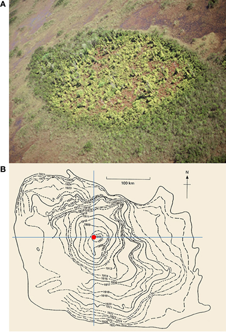
Figure 1. (A) An example of new invasions of Old World climbing fern (Lygodium microphyllum) at the patch-level in the greater Everglades ecosystem of southern Florida, USA (photo courtesy S. Miao). (B) The historical spread of muskrats (Ondatra zibethicus) at the range-level in central Europe from 1905 to 1927 (after Elton, 1958; see also Shigesada and Kawasaki, 1997).

The invasion of an exotic species typically starts from either the location where it is first introduced or the established distribution or “abundance centers”(C) (Sagarin and Gaines, 2002) that host the concentration of its individuals within the invaded ranges. At the range margin (M) (also called species' borders, boundaries, range limits; Gaston, 2003), the species form invasion fronts with highly dynamic, sensitive, but usually smaller populations (Holt and Keitt, 2000). By connecting the populations between the center (C) and margins (M) through meta-population processes (Moilanen and Hanski, 2001), many population parameters and associated variables such as growth rate and survivorship form detectable C-M patterns and gradients (Guo et al., 2005; Alexander and Edwards, 2010). To better understand the effects of global change on invasion and to develop techniques that can be used effectively to manage invasive species, we need a better understanding of the population dynamics along the C-M gradients (Figure 2) and the associated processes and mechanisms. For example, global change in climate and land use may have coupled or interactive effects on the population dynamics (i.e., spreading or migration) of alien species (Malchow et al., 2008; Mistro et al., 2012); that is, (1) climate and land use changes may act as disturbance agents, opening up patches for invasives to colonize and form new marginal populations (Hobbs, 2000), and (2) climate warming and increased extreme events may promote the invasion of alien species that prefer disturbance and higher temperatures under which many native species cannot compete (Huston, 2004; Olatinwo et al., 2013).

FIGURE 2

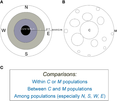
Figure 2. (A) A graphic representation of an idealized species' range in which population density declines from the range center (C) to margin (M). (B) The average patch size or population size decreases from center to margin but isolation increases. (C) Examples of common comparative strategies within, between, and among populations across species' ranges (e.g., Bakker et al., 2006; Soley-Guardia et al., 2014). For marginal populations, between (N-S, for example) and among-population comparisons can be made in four major directions (N, S, W, and E).

Geographically, an ideal location to monitor species invasions would be at the species' borders (or range limits). This is mainly because marginal populations are most sensitive to environmental changes due to the short history of colonization and smaller sizes (Keitt et al., 2001). The dynamics of these populations would serve as a good indicator regarding the direction and speed a species is invading or spreading under changing climates and land use scenarios (Watts et al., 2013). However, marginal populations as “sinks” (Dunning et al., 1992) often cannot act alone as they reply on central populations as “sources” for new colonization, persistence, and further expansion through gene flow and immigration (Guo et al., 2005; Eckert et al., 2008). Therefore, comparisons and exploring the connections between central (C) and marginal (M) populations would be necessary and are one of the most powerful and efficient approaches to study species invasions. This is particularly the case when time and resources do not allow the whole-range monitoring and assessments. Nevertheless, despite great efforts in searching for life history, genetic, and functional traits that may be responsible for species invasiveness, at the population level, whether an invasion can succeed is determined by four vital rates, i.e., birth, death, immigration, and emigration.

Traditionally, most central-marginal (C-M) comparisons have been conducted on native species, especially for conservation purposes (e.g., Channell and Lomolino, 2000; Angert, 2006; Yakimowski and Eckert, 2007; Angert et al., 2008; Eckert et al., 2008; Doak and Morris, 2010; Hardie and Hutchings, 2010; Belyayev and Raskina, 2013; but see Mandak et al., 2005; Leger et al., 2009). Earlier findings from such comparisons include that central populations are larger, more primitive, and more stable than marginal ones (e.g., Williams et al., 2003). However, such overly simplified approach has several limitations. For example, many patterns and processes from C-M are often nonlinear. Also, populations at different margins (directions) often exhibit drastic differences in structure and dynamics. Therefore, simple C-M comparisons could not reveal a complete picture of population structure and dynamics across the entire species ranges (Fenberg and Rivadeneira, 2011) and consequently the underlying mechanisms. For example, some recent comparisons across three spatial categories (i.e., central-middle-marginal) found some unique features in the populations located between the center and margins (or “middle” populations). In other words, some population parameters are not simply the mean averaged between C and M populations (e.g., Vallecillo et al., 2010).

Partly due to the unprecedented rise of bio-molecular technology, there is an apparent shift in literature from traditional and direct C-M comparisons (such as population density, growth and reproduction rates per capita, and transport coefficients) to whole-range-level assessments of genetic diversity associated with the C-M gradients (Eckert et al., 2008). The former is mostly devoted to basic ecological research, and the latter is increasingly linked to climate change (e.g., population migration during the retreat of last glaciation and ongoing climate warming) and habitat fragmentation (i.e., isolation due to land use). However, ecological and genetic factors are closely related to each other that interactively regulate population dynamics over both space and time (Magurran, 2007). For example, for many species, climate conditions can limit species distribution, but whether the species can expand its range (birth > death) could be affected by the genetic flexibility and evolutionary potential of its component populations, especially those at the margin (Holt and Keitt, 2000).

Recently, a few studies have applied the C-M model to invasive species (e.g., Alexander and Edwards, 2010). While by intuition that the C-M model developed for native species may be equally applicable to invasive species, it is critical to make a clear distinction between applications of C-M in native vs. invasive species. Compared with many native species that are relatively stable or shrinking in abundance and distribution due to habitat fragmentation, invasive species are still spreading at high rates and their initially formed abundance centers are still relatively intact. This is especially the case for invasive species for which management and eradication, even at the local scale, have to date not been successful. In addition, exotic species are often introduced to various locations thus form multiple initial abundance center. With its continued spreading, the abundance center will migrate until the exotic range stabilizes. Thus, for invasive species, the C-M processes are highly dynamic and the patterns are more time-dependent. For these reasons, it is possible that C-M may be more applicable to invasive species. Certainly, additional insights could also be gained from comparisons of C-M patterns of the same species between their native and invaded exotic ranges.

The presence/absence and dynamics of a population at a specific location (patch) with a species' range and a specific time are ultimately determined by its overall performance balanced among birth, death, immigration, and emigration. As C-M patterns and processes are tightly linked to the species' abundance centers, range limits, range (and patch) geometry (i.e., size, shape, fractal dimension), and genetic variation across its ranges, I examine the C-M population dynamics of invading species based on the following premises: (1) clear distinction between invasive species (fast-spreading: “birth > death, immigration > emigration”) and natives (relatively stable: “birth ≈ death” or even contraction to become rare species: “birth < death, immigration < emigration”), (2) more emphases on hierarchically nested patches within species ranges (i.e., populations in small patches nested within larger patches) and the range-patch relationship, and (3) the increasing effects of climate/land use changes (e.g., “source-sink” shifts and associated species migration). I also discuss the importance of more comprehensive sampling and questions for future research. Clearly, different from studies on natives are for conservation (especially rare/endangered due to range contraction), the research for exotic species (especially invasives) are intended for better management (due to rapid range expansion).

Generality of the Abundance Center

The abundance center concept is nebulous, and its association with Gaussian curves has recently been challenged based on some studies on native species (Sagarin and Gaines, 2002; Kluth and Bruelheide, 2005; Yin et al., 2005; Lester et al., 2007), although evidence of support also continues to accumulate (e.g., Whittaker, 1971; Brown, 1984; Feldhamer et al., 2012). Indeed, pinpointing an abundance center for a specific species is often subjective and debatable and the magnitude of abundance center varies among species. There are several main reasons for this. First, a criterion for defining a commonly acceptable concept of abundance center has never been in place. Second, the sampling techniques and measurements of abundance also vary drastically among researchers, species, and even across the different parts of the same species' ranges. For example, for the same species, the window (plot, quadrat) size, sampling time, and associated procedures (e.g., averaging, smoothing; Gaston, 2003) could change the abundance curves significantly. Third, the species ranges and population dynamics of many species are highly dynamic (from year-to-year, season-to-season), especially with the unprecedented habitat destruction by human activities. While it is true that more comprehensive survey across the whole species ranges would help resolve this issue, a clear and commonly acceptable criterion for defining “abundance center” is needed (e.g., how strong a center can be called a “center” and how smooth the abundance curve has to be).

However, although abundance curve has often been described as Gaussian, normal, or bell-shaped for simplicity in theoretical and modeling studies, species rarely show perfect smooth and symmetric curves in abundance (Samis and Eckert, 2007). The deviation from Gaussian distribution can occur in a simple model if the resource distributions are not homogeneous (Ryabov and Blasius, 2008). Species with linear distribution such as those along coastlines or riparian species might be treated as special case because, relatively, the number of such species is much lower than other species. Different sampling strategies are often used for such species because of their special (narrow) range-shapes. The switch of the margins of the same species across different times of observation makes pinpointing or even estimating the actual range limits difficult (see Fortin et al., 2005).

Intuitively, every species would have an abundance and/or distribution center at some point or across some stages in its history, especially newly emerged or colonizing species (e.g., invasive species). When abundance center is loosely defined, any species with an aggregated distribution should have abundance center(s). However, over time, the original or older abundance or distribution centers can be relocated and reestablished as species migrates, and destructed due to habitat fragmentation. Moreover, the abundance centers are not often located in the physical center measured using Euclidean space. Studies using contour (density) maps where detailed numerical information is not available often show abundance centers when density within each abundance interval (or between lines) is averaged. In some other cases, however, species reaching physical barriers such as coastal lines usually do not represent species “niche” position or the full extent of physiological responses (Brown, 1984; Gaston, 2003; Dawson et al., 2010; but see Holt and Keitt, 2000). Brown (1984) and Gaston (2003) outlined several factors that can cause the “exceptions” or “extreme cases,” including abrupt physical barriers such as sea-land boundaries (e.g., coastal species), farmlands, clear cuttings can interrupt species distribution although other factors such as climate are favorable (in such case, the true or potential abundance center may not show). Allee effects (threshold) may also be responsible for many species range limits where clear change in environmental gradient is absent (Keitt et al., 2001). Dispersal is another leading factor that could cause either gradual or abrupt species range limits.

For species with clear abundance centers, the entire ranges would cover a cohesive core and many isolated or less connected marginal populations. The same invasive species would form multiple abundance centers when introduced to multiple locations in addition regardless whether abundance center exists in its native ranges. Over time, from the origin to extinction and one side of its range crossing its favorite environment to the other side of the range, a species almost surely experience the rise and fall of abundance. However, similar to abrupt spatial patterns, species may suffer sudden extinction as well (due to volcanic eruption, extreme climate change, or effective control/eradication in invasive species cases; for example), forming abrupt temporal abundance curves.

C-M Variation in Population Size and Density

Variations within and among populations are critical for understanding species-range structure and dynamics (Storey et al., 2007; Bertocci et al., 2011; Guo, 2012). Both population size and density are main elements reflecting population structure and dynamics. Where abundance centers exist, the central-marginal hypothesis (CMH; Eckert et al., 2008) which predicts a C-M decline in population size and density may apply. In recent years, we have seen a remarkable shift from dichotomy to continuum in comparisons across populations within a species' ranges. For example, using theoretical simulation models, Guo et al. (2005) described population dynamics along the numerical abundance (density) gradients from center to margins. The “continuum” approach is necessary to help detect the existence and/or strength of spatial (auto)correlation and population synchronization (synchrony-distance relations) across the species' ranges (Liebhold et al., 2004a,b).

There are more studies that have specifically focused on marginal than central populations (i.e., effects of marginality; e.g., Grant and Antonovics, 1978; Furlow, 1995; Mandak et al., 2005; Kawecki, 2008; Belyayev and Raskina, 2013). Several reasons make studies on species' borders intriguing: (1) marginal populations are more sensitive to environmental changes, (2) marginal populations can indicate that a species' ecological requirements are in equilibrium with properties of the environment (Hengeveld, 1990), (3) species borders discriminate best between conditions favorable for the species and those that are not, (4) marginal habitats provide ideal sites to study species interactions (competition, hybridization, predation; e.g., Whitham et al., 1999), and finally (5) marginal conditions can indicate potential ranges for species invasion and species transplantation. Although many invasive species have been intensively studied (see next section), the role of dispersal and other causes for their high invasiveness associated with its boundary shifts and the practical implications of such boundary changes have not been adequately investigated.

To characterize the dynamics of hierarchically structure populations across a species' range, the first step is to examine the spatial extent of individual populations and spatial variation in population density (i.e., number of individuals per unit area). In contrast to most studies that compare central and marginal populations only; it would be more meaningful and now feasible to compare the populations located within various distance intervals along the C-M gradients (Figure 2). For a species with a roughly circular range (see Guo et al., 2005), when a species' range or patch is divided into a number of rings (j) or compartments from the center to margin, the size of all populations in the ring, is N_j = n_jA_j, where A_j is area and n_j is population density in the ring:

$N_j=n_j\pi (x_{j+1}^2-x_j^2),$

where x is the distance from the center of the species' range. For heuristic reasons, the number of populations per ring was calculated under two density distribution scenarios, Gaussian-like and uniform (or random). Under the Gaussian scenario, the population density (n_j) is

$n_j=a{e}^{-e{x}^2},$

where a is the population density at the range center and c is the rate of density decline with distance. Under uniform (or random) distribution, the total population in jth ring would be: a*A_j. Assuming there is a positive relationship between population size and genetic diversity, the total population size would be highly correlated with the overall genetic diversity in each ring, and the curve of the total population size (i.e., all individuals in each ring) across the rings would indicate how total genetic diversity changes from the range center to the margin.

In these overly simplified models, the ring itself does not have any specific biological meaning; rather, its location and relative position within the species range indicates the population density, population size, and the possible directions of gene flow among all the populations inside the ring relative to those in other rings across the whole range. However, in reality, the positions of the rings should reflect the changes in actual population density associated with resource availability (Ryabov and Blasius, 2008), the number of populations, or the geographic patterns of population presence from the center to margin (i.e., a contour lines), rather than being arbitrarily assigned with a regular circler shape.

The ranges of many natives have much longer history and suffer range destructions such as habitat loss and fragmentation caused by human activities, losing typical abundance centers (Fordham et al., 2013). However, for invasive species that are spreading with high speed (b > d), Gaussian pattern is likely to better describe their abundance, especially the patches within species ranges, and examples of such spreading invasives are numerous (e.g., Lygodium microphyllium; Figure 1). Therefore, it may be more appealing to apply the abundance center theory to fast expanding invasive species after forming abundance centers at the original locations where they are introduced and established. That is, many principles regarding the C-M gradients may still apply.

Central-Marginal Phenotypic and Genetic Variation

Species vary greatly in adaptive ability (flexibility) or resistances to environmental changes. Usually, central populations have a reduced sensitivity to environmental change due to their larger population size (cf. Grant and Antonovics, 1978) but they may show greater within-population diversity (both genetic and morphological), whereas marginal populations would show greater among-population variation because they are smaller and more isolated and suffer higher extinction risks. Asymmetrical gene flow from the center of a species' range may prevent adaptation of marginal populations and consequent range expansion (Reichert, 1993; Bridle and Vines, 2007).

Most studies on central-marginal or range-wide genetic structure across species' ranges have been performed on native species for establishing conservation priorities, coincident with unprecedented biodiversity loss and global climate change (Eckert et al., 2008; Guo, 2012). Very little is known about the genetic variation of invasive species, hindering our efforts for invasive species management. Studies on invasive species have mainly focused on general ecology, physiology, morphology, and more recently, molecular biology; however, no genomics technologies have been applied to investigate invasive species invasiveness from ecological perspectives. It is expected that the genetic structure and flexibility could affect population dynamics. A study of gene expression in conjunction with an analysis of genetic changes occurring since introduction and in relation to adaptation to soil and climate factors will provide important information for early prevention.

Some species may not evolve noticeably over millions of years while others may show genetic restructuring in decades. Analysis of genetic information can provide powerful insights into the origins, history, and genetic drift of invasive plants. A quantitative comparison of genetic information of a plant in its native habitat and its colonized habitat can suggest the rate and type of evolution taking place in both populations. While studies so far on habitat invasibility and species invasiveness have been largely focused on physical factors (i.e., disturbance, climate change) and morphological features (i.e., dispersal, competition, growth rate), the critical information on how species can adapt to or exploit a new environment through genetic changes is mostly lacking. However, for many invasive species, adaptability could be the cause of their high invasiveness.

For species with declining density from range center to margin, if the positive relationship between population size and genetic diversity holds, higher genetic diversity is expected in an individual central population than in a marginal population. However, when all populations in each ring are considered, the majority of individuals of the species actually exists in the intermediate area along the C-M gradients, despite the highest population density at the center (Figure 3, top). The populations in the middle, as a whole, would receive greater inputs (gene flow) and asymmetrical feedbacks from both central and marginal populations and thus may hold the greatest amount of genetic diversity of the species, although the diversity per population or per unit area is still the highest at the center. This enhanced diversity may contribute to genetic variation and stability to central but especially to marginal populations through asymmetrical C-M gene flow. Less commonly, when a species has a uniform (or random) distribution in density across its range, most individuals of the species are located in the marginal habitats due to the overall larger area the species occupies (Figure 3, bottom).

FIGURE 3

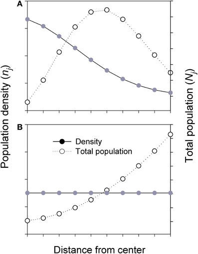
Figure 3. Simplified diagrams showing the population density (n) and total population size (N) in each ring (i.e., sum of all populations) across the whole species range or a patch (i.e., from center to margin). N_j = n_jA_j; where A_j and n_j are the area and population density in jth ring, respectively. (A) Total population (all populations in each ring) is estimated based on Gaussian-like distribution of population density across the species range or a patch. (B) Total population is estimated based on uniform or random of population density across the species range or a patch.

The majority of previous studies is based on analyses of neutral markers, and suggest greater genetic diversity in central rather than in marginal populations, but other studies have found the opposite or no clear pattern (Eckert et al., 2008; Saavedra-Sotelo et al., 2013). Both empirical and theoretical evidence also show positive relationships between population size and genetic diversity (Frankham, 1996). The inconsistent results and ensuing debates may have multiple causes related to the interactive effects of: (1) history or phylogeography (Pouget et al., 2013) such as events related to the advances and retreats of glaciation, (2) the effects of range geometry and orientation, and (3) variation within single vs. among populations. Other related contributors may include: migration, isolation, species age, and geographic positions of the populations in the species' range.

For most species, a few larger central populations occupy a smaller area around the center of the species' ranges and are geographically closer to each other. As a result, gene flow among these central populations would be greater and more symmetrical, thus reducing differentiation among populations (e.g., Wakeley, 2004). In contrast, numerous but smaller marginal populations surrounding the central populations and other interior populations occupy a much larger area and are relatively more isolated from each other, especially from populations on the opposite sides of the range. In most case, the genetic diversity within each marginal population is generally lower than that in central populations (Eckert et al., 2008; Guo, 2012). The greater isolation not only reduces gene flow from central populations (“sources,” often asymmetrical) but also greatly reduces gene flow from other marginal populations (“sinks”), thus increasing the genetic differentiation among marginal populations. For species with either a Gaussian or uniform distribution, central populations are surrounded by neighboring populations (large and small) in all directions. However, marginal populations occupy a smaller portion of their borders (<50%; Figures 2, 3) with neighbors of its own species (i.e., the populations located in the middle between center and margins; usually smaller) to exchange genetic materials (gene flow), which could reduce their genetic variation. For species with a uniform (or random) distribution, the genetic diversity within interior populations would be similar across the species' range because of similar population sizes and distances among populations. Epperson (2007) recently tested how population size, dispersal, and distance are interrelated and how they together affect spatial population genetic structure.

The simplified C-M models in Figure 3 clearly have limitations as they do not apply across all taxa and to species with unique distribution patterns or extremely small ranges (e.g., extremely rare species with very few individuals; see also Gaston, 2003). Species with special or unique distributions as a result of physical boundaries (e.g., coastal species; for an example of truncated species range; see Howes and Lougheed, 2008), species introductions or biotic invasions, and disjunctions due to habitat fragmentation (see Le Roux et al., 2008) deserve special treatment. The models in Figure 3 only concern spatial pattern; the temporal fluctuation in populations along the C-M gradient related to disturbances and population age needs additional attention. In addition, human-related factors could significantly complicate or erode the positive relationship between population size and genetic diversity (Paetkau et al., 1998).

Populations at the northern (N), eastern (E), southern (S), and western (W) limits and the center are likely to experience very different physical and biotic conditions and thus different selection pressures. As a result, genetic structure would be different among these populations, especially between N and S populations that may experience the warmest and coldest temperatures within the species' range (cf. elevational diversity patterns on different aspects of the same mountain in the temperate regions), even if the range limits of species are not limited by climate. Also, where latitudinal decline in species diversity from S to N (in northern hemisphere) within a species' range is detectable, S-populations would interact with more species thus greater forces of selection against the species than N-populations. In such cases, the commonly observed C-M decline in within-population genetic diversity would be overshadowed by the overwhelming S-N declining trends. For example, Howes and Lougheed (2008) sampled the whole species range of a temperate lizard (Plestiodon fasciatus) and found that the species showed a gradual decline in genetic diversity from S to N populations.

Recent literature increasingly has focused on the effects of climate change on population migration and range shift (e.g., equatorial/downward vs. poleward/upward). There is little discussion on the importance of possible longitudinal trends. Nevertheless, if the W and E populations encounter dramatically different environments (e.g., mountains at one end vs. coasts at the other), they might make unique and important contributions in overall genetic diversity of the species (e.g., Howes and Lougheed, 2008). In such cases, averaging the genetic variations (patterns) in all directions would almost certainly overshadow the C-M patterns because the marginal populations in very different conditions are likely to harbor unique or novel genes or genotypes. These additional factors that have not received deserved attention might also help explain the inconsistencies and complications in previously reported C-M patterns (see review by Eckert et al., 2008).

Invasion biology is increasingly taking the advantages of fast advances in molecular biology. For example, microarray technology works on the principle that cognate nucleic acids hybridize with each other, and it allows us to systematically evaluate the expression pattern of large subsets of genes in given tissues over multiple developmental stages and in response to various environmental stimuli (Chao et al., 2013). The focus on microarray analysis includes, but not be limited to determination of environmental factors and genetic makeup involved in adaptation and invasiveness of exotic species from the center (i.e., central populations) to its borders (i.e., marginal populations). Again, to do this, it would be necessary to make comparisons between old (core) and new (marginal) populations, and between native and introduced regions to see if species have changed significantly in genetic structure since introduction.

To determine physiological responses and adaptations to specific climatic conditions that affect the spread of invasive species, populations from the northern (or upper) and southern (or lower) limits of the range as well as populations in the center of the range will be identified. A pool of individuals should be randomly selected from each population. These clones will be subjected to various treatments including, but not limited to, high and low light intensity, cold/heat stress, drought stress, and nutrient stress. Plants will be harvested and tissues from roots, stems, leaves, flowers, vegetative buds, and seeds will be separated and RNA from these samples will be extracted for future studies. Microarrays will be used to establish the gene expression patterns characteristic of each population in response to these stresses. A comparison of gene expression patterns between the ecotypes under stressed and nonstressed conditions should provide an indication of physiological responses and the diversity and intensity of specific stress response pathways of invasive species.

Description of species distribution patterns is often complicated by species with “special” shapes such as coastal, riparian, and lake shore that may be linear, curved or highly irregular and fragmented (Schmeller et al., 2005). Perhaps a special category needs to be established although one dimension (cross the width of the linear range) may still follow the C-M pattern. For species with linear ranges, range orientation is an important factor. If a species has N-S oriented range with a considerable latitudinal extent, S populations might show higher genetic diversity than C and N populations. In contrast, if a species has a range with a dominant W-E orientation, the C populations may still hold the highest genetic diversity, unless strong longitudinal environmental gradients such as elevation are present (Guo, 2012). But again, the highest genetic diversity per population or per unit area would still be located at the center (core) unless a strong S-N declining gradient exists (usually for species with broad latitudinal extents) because it is the only place where all cardinal directions come together in the same set of populations.

Scale and Hierarchically Nested Patches within Species Ranges

Many species actually have multiple abundance centers. Typical examples include the native species with disjunct distribution, either within or between continents. Species introductions by humans form many more disjunctions thus many new abundance centers. For example, some 80 native plant species and over 900 introduced plant species have disjunct distributions between North America and eastern Asia (Guo et al., 2006). Even in the same region (native or exotic), the original abundance center could disappear due to disastrous infectious diseases or human land use (e.g., farm lands; Bahn et al., 2006). Given that much of the earth's surface already has human footprints, the range-level abundance centers of many native species might have broken into many smaller center across patches hierarchically embedded within species' ranges (Kokko and López-Sepulcre, 2006; Samaniego and Marquet, 2013). On the other hand, species invasions to new locations often form multiple new patches within the species' ranges (Figure 1, top).

The abundance center may occur at any scale, ranging from small patches to the entire species' range. At larger scales and for many species we still do not know how genetic diversity is apportioned within and among populations across the whole ranges. A growing body of literature based on both empirical and theoretical evidence continues to show the positive relationship between population size and genetic diversity (Lammi et al., 1999). If the positive relationship between population size and genetic diversity holds broadly across species and geographic localities, we should examine the spatial distribution of population sizes across a species' range first. However, the results are likely influenced by species-range geometry as I have shown, ways of comparisons, and sampling procedures as detailed below.

Species' range expansion, contraction, or migration can also be reflected by changes in patch occupancy within a species' range. At smaller scales within species ranges, landscape structure (e.g., patches) can affect the evolutionary processes such as gene flow and mutation particularly at the patch boundaries. However, like many landscape features, a species range is often fractal with many patches hierarchically nested within the range and the “central place theory” may be applied (Milne, 1991; Forman, 1995; Wu and Loucks, 1995; Chen and Zhou, 2006).

Alternative approaches should be considered and adopted in some cases. For example, a model developed by Borgatti and Everett (1999) for the core/periphery structure in social networks could be used for studying central-marginal population structure and dynamics. The model is based on the connectedness (ρ) among all nodes in the network.

$\begin{array}{l}\rho ={\displaystyle \sum _{ij}{a}_{ij}}{\delta }_{ij}\\ {\delta }_{ij}=\left\{\begin{array}{c}1if{c}_i=COREor{c}_j=CORE\\ 0otherwise\end{array}\right\}\end{array}$

where a_ij indicates a link (absence or presence) in the observed data, c_i indicates either a population belongs a core or periphery, and δ _ij is a pattern matrix indicating the presence or absence of a link in the ideal or maximally centralized pattern (Figure 4). In this model, instead of testing whether a single abundance center exists, the network analysis or centrality measure examines how close (approximation) between the observed data (nodes) and an ideally connected structure. The central nodes or populations could act or be treated as “attractors” in chaos theory (Borgatti and Everett, 1999; see also Gleick, 1987). Such models have limitations of giving equal weight to each link present. Nevertheless, new network analysis tools are being developed that would soon overcome these drawbacks.

FIGURE 4

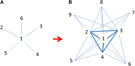
Figure 4. (A) Initial invasions at time t when marginal populations are only linked to central populations (Freeman's star; Freeman, 1979); (B) Continued expansion of established populations across species' ranges at t + 1 after initial invasion when many populations are increasingly linked to each other but mostly to central ones (revised following Borgatti and Everett, 1999). Both graphs are idealized patterns designated for approximations using observational data. Numbers indicate the emerging sequence of populations (nodes) over time; i.e., smaller numbers are older and more centrally located and interconnected.

Imagine a small population located around the geographic center but remains ecological isolated (i.e., weakly linked to others) for some reason. Such populations would not function like other central (or core) populations. On the other hand, populations of rare species become increasing separated due to habitat fragmentation whereas those of invasives are becoming increasingly connected among each other (Schooley and Branch, 2011). Because population dynamics would be more relying on what happens not only in the target populations, but also in the ones that they are connected to each other, management should consider well-connected populations and those isolated separately.

The Role of Range Shape, Orientation, and Boundary

Species ranges show diverse and dynamic sizes, shapes, and orientations that can profoundly affect the direction and amount of gene flow thus spatial variation in genetic diversity within their ranges. For simplicity, the circular or near circular shape and linear or near linear shape have often been used to study range and population dynamics, especially in theoretical research (e.g., Guo et al., 2005; Watts et al., 2013). In Both range-shape types are loosely defined, with the former exemplified by the strong correlations of populations in many species between the latitudinal (N-S) and longitudinal (W-E) dimensions (Brown, 1995), and the latter is exemplified by coastal or riparian species which tend to be somewhat linear and restricted in width (Sagarin and Gaines, 2002). It is difficult to categorize and quantitatively analyze species' ranges that have highly irregular shapes, such as ranges that encompass continents and islands. To characterize such complex range shapes, more sophisticated tools are needed. A parallel issue also exists in describing density functions within species ranges. Among the most frequently used density functions along C-M gradients is the Gaussian-like pattern (or density-decay function from the center). Random and uniform functions have theoretical values in theoretical and simulation studies but rarely occur in nature especially at the whole-range level (Murphy et al., 2006).

As shown above, even for species with circular or near-circular shapes, comparison and sampling strategies can be conducted in a variety of ways and some of the inconsistencies in early studies may be due to the effects of geometry. Indeed, traditional comparisons between central and marginal populations, especially those based on one cardinal direction only, clearly have not taken the species range shape (geometrics) into account. Because of the different ways of comparing among populations even just between central and marginal populations (Figure 2C), different conclusions could be reached. For example, for species with a Gaussian-like distribution in population density, if we compare a pair of populations, one at the center and the other at the margin, we may find greater genetic diversity in the central population. When a population at the lower latitudinal limit is compared with one at higher limit, the former usually shows higher genetic diversity (Guo, 2012). However, when all central and marginal populations as two contrasting groups are compared, marginal populations might hold higher overall genetic diversity than central ones. When all populations in each distance interval (ring) from the center are considered, the populations in the intermediate area between center and margin hold the majority of the species' genetic diversity (Figure 3).

Range boundary is a sensitive indicator of species expansion or contraction in response to environmental changes. It may be regulated by dispersal capability, physiological tolerances, and interactions with other species, among others (e.g., Holt and Keitt, 2000; Fortin et al., 2005). Most studies have examined temporal dynamics of local populations. It is unclear, however, how spatial differences in birth rate, genetic structure, dispersal, and interactions with other neighbor species can affect species' range expansion, contraction, and/or migration (Guo et al., 2005). More generally, With (2002) has suggested that landscape structure, by influencing dispersal, demography, and species interactions, plays a large role in determining invasive species abundance-distribution relations (e.g., Figure 5) and spread.

FIGURE 5

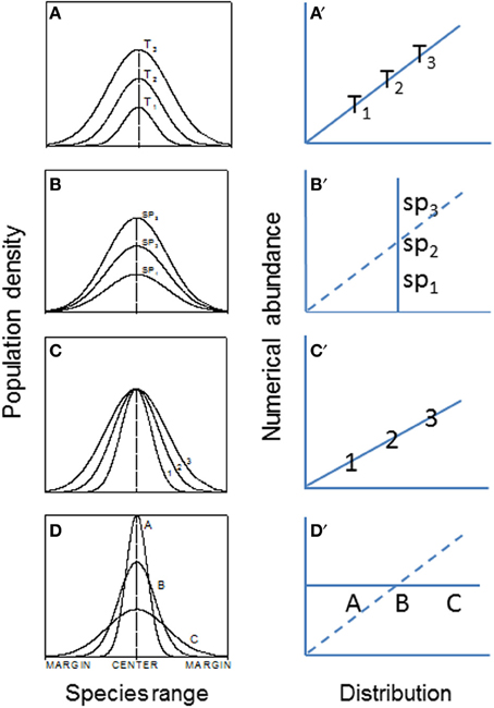
Figure 5. The hypothesized patterns of abundance (population density) and abundance-distribution relationships across patches or species ranges (Veldtman et al., 2010). (A) The most common form where both abundance and range simultaneously increase with time, i.e., habitat and climate conditions are not limiting in the invaded ranges (e.g., the historical spread of muskrats, Ondatra zibethicus, in central Europe; see Figure 1). (B) Habitat area is highly limited but climate conditions are favorable. (C) Habitat area is not limited but climate is. (D) Combined scenarios of (A–C). The right panels (A′–D′) are corresponding relationships between abundance and distribution.

In conservation biology, the minimum and optimum areas are identified and protected so that minimum population sizes of a rare species can be maintained. The same logic may apply to managing or eradicating invasive species, i.e., by breaking the ranges or patches into small pieces so that the populations can be isolated and eventually brought under control. The shape of the area and the locations in relation to the center and margin of the focal species' ranges must be important considerations because they will greatly influence spatial processes such as dispersal, migration, pollination, hybridization, and infestation by pathogens (Harris, 1988). More importantly, all these actions should be guided under the current and projected global change scenarios. Habitat and invasive species modeling using remote sensing-GIS facilitates the development of broad-scale, contextual, and predictive models (Peterson and Vieglais, 2001). The potential of these modeling tools regarding invasion prediction, mitigation, and management is largely unrealized.

Abundance Curve as Indicators of Species Migration and Climate Change

Many species including invasive species migrate due to climate change (e.g., Guo et al., 2012; Bertelsmeier et al., 2013; Figure 6). When subjected to environmental changes, a population can avoid extinction either by adapting genetically to the new environmental conditions or by tracking its old environment across space (Pease et al., 1989). However, under certain conditions, demographic and genetic contributions from conspecific immigrants tend to reduce extinction rates of insular populations although, occasionally, migrations from “sinks” to “sources” could also occur (Figure 6). All these changes in population parameters associated with climate change can be reflected in the shifts of abundance curves over time (Figure 7).

FIGURE 6

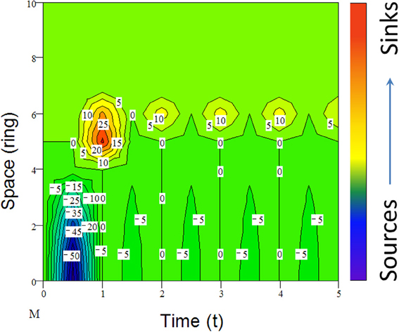
Figure 6. An example of simulated population dynamics across space from center (bottom) to margin (top patches) and time (reproductive seasons). For active migrants (mostly animals), long-distance dispersal (e.g., leptokurtic) could lead to the establishment of “pocket” populations (top) with long-persisting certain genotypes (Ibrahim et al., 1996). Positive numbers indicate the immigrants from the “source” or center and negative numbers (density) are the emigrants to the “sinks” or margin, following the active migration function (M) from jth to ith ring (ith ring is located outside of the present range in Figure 2; for details, see Guo et al., 2005).

FIGURE 7

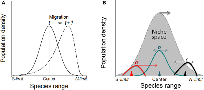
Figure 7. (A) Without physical barriers, the deviation of the abundance curve of a species from Gaussian distribution may indicate the migration direction under warming climates (in northern hemisphere; e.g., Maggini et al., 2011). Here, the population or the whole species range is moving toward the left where the abundance curve shows a much steeper slope than the right side. (B) The direction and magnitude (indicated by the arrows and their lengths, respectively) of shifts in abundance depend on where in the niche space the species is introduced (i.e., the positions of triangles) as shown by three newly introduced species as examples (a–c) although the niche space may also shift poleward under climate warming.

It is expected that the specific genetic structure of the central and marginal populations of different directions as a regulator would make differences in population dynamics (Eckert et al., 2008). Under human induced climatic warming, species will show elevational (upward) migration from continuous distribution at lower elevation to mountain tops thus form multi- and smaller distribution/abundance center (Lomolino, 2001). Smaller patches formed as a consequence of climate warming may become less stable as reflected by rapid changes in patch area and shape, and population structure would change as well. Historical data (e.g., museum collections) or abundance curves drawn at different times would be needed to solve this problem because it only makes sense when current abundance curve is compared with the historical ones to make predictions on population or species migration (see Figure 7, left). Similarly, the location of first introduction of the invasive species in the entire niche space would indicate where and how fast the species may further invade under both present and projected climate changes (Guo et al., 2012; Figure 7, right).

Similar to simulating the spread of human infectious diseases which mainly depends on the effective distance and rate of spread (e.g., Brockmann and Helbing, 2013; Nelson and Williams, 2013), the spread of invasive species could also be a simple reaction-diffusion process across the invaded and potentially invasible regions. Like many theoretical models, the assumptions in C-M models not necessarily realistic and complete; rather, they are intended for modeling simplicity to identify major ecological (demographical) drivers in population/range dynamics. A new species may often show a Gaussian curve but a newly introduced species may show deviations depending on where the species is introduced in its potential range. In nature, no species really has a perfect, smooth, symmetric, Gaussian curve. It is always helpful to question how realistic a theoretical model may be. Like many theoretical models, our assumptions not necessarily realistic and complete; rather, they are intended for modeling simplicity to identify major ecological (demographical) drivers in population/range dynamics. A new species may often show a Gaussian curve but a newly introduced species may show deviations depending on where in its potential range the species is introduced. Indeed, exceptional cases deserve special attention and need specific and additional work. In most cases, we are dealing with common patterns. Historical data or abundance curves drawn at different times would be needed to solve this problem because it only makes sense when current abundance curve is compared with the historical ones to make predictions on population or species migration (see Figures 7, 8).

FIGURE 8

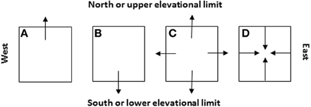
Figure 8. Four likely scenarios of the species' patch or range dynamics in major cardinal directions (i.e., A: shift northward, B: shift southward, C: expansion, and D: contraction) and their dependence on the initial locations of species introduction relative to the niche space and future climate change (see Figure 7). These cardinal directions are selected because they represent (1) the latitudinal gradients (S-N) along which the glaciations took place in the geological past and climate warming occurs and/or (2) the distance to the oceans or elevational changes (E-W, e.g., across North America or eastern Asia).

Simulation and Geospatial Modeling

Existing studies of invasive species have typically relied on methodologies associated with conservation biology, with limited development of the broad-scale geographic context and limited application of geospatial technologies. Given the complexity and multi- dimensions (spatiotemporal and human) of many species (Oro, 2013), geospatial simulation continues to be a pivotal tool, especially for projections of future population trajectories. After identifying and mapping the ecological features on invasive species' native regions, we can use simulation modeling (incorporated with projected future climate changes), GIS-remote sensing technology, and ecoinformatics to identify the potential habitats and directions of invasives future invasions in the invaded regions (e.g., Albright et al., 2010). Some invasives have distinctive characteristics in degree-days, soil temperature, elevation, and modeled evaportranspiration that may be used in combination with remote sensing to model distribution probabilities of the species (Underwood et al., 2003).

Previous modeling/simulation efforts on (marginal) population dynamics, adaptation and gene flow have used both deterministic and stochastic models including stepping-stone, source-sink, reaction-diffusion, and network models, among others (e.g., Antonovics et al., 2001; Keitt et al., 2001; Alleaume-Benharira et al., 2006). Each model shows advantages and limitations by addressing certain features while ignoring others. Because of the complexity and the large number of factors involved, a holistic or integrated approach simultaneously incorporating most if not all the critical features in one model seems impractical or almost impossible. On the upside, many new epidemic models are being developed for simulating and predicting the spread of infectious (human) diseases (e.g., Nelson and Williams, 2013) which could be adopted for invasive species because of the analogs between the two areas/subjects.

Sensitivity analysis predicts that central populations (or patches) are more stable, both spatially and temporally, while marginal populations (or patches) are more sensitive to environmental changes, especially for species with great dispersal power (Figure 9). To test this prediction, one may compare patches at the range center with similar sizes to those close to range margins to determine whether the population size or boundary changes are of a smaller magnitude than those of marginal populations. It would be reasonable to assume that patches within the invaded range will respond similarly to the whole invaded range, i.e., expanding, contracting, or shifting, following climate or land use changes. By combining the survey data from selected patches across the invaded range, we would be able to determine the level of synchronization in patch size dynamics and the direction of these changes (e.g., poleward or equatorward; see Figures 7–10). In either case (population dynamics synchronized or not synchronized), monitoring multiple patches across the invaded range will provide valuable information as to how climate might affect species invasions.

FIGURE 9

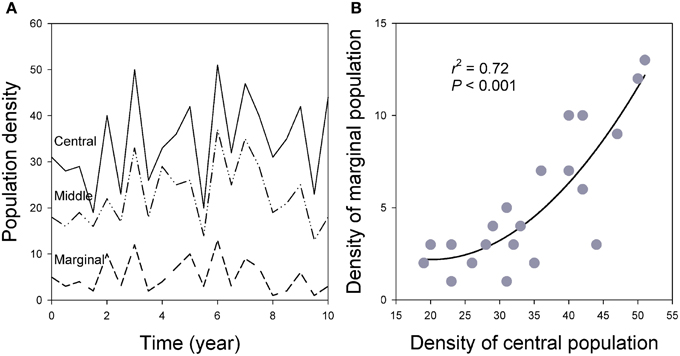
Figure 9. (A) Population synchronization across the species' ranges in which marginal populations show greater variation measured by CV of population density over time. (B) Population densities are closely related between central and marginal populations over time as the result of spatial synchronization (see also Figure 6; for details of the simulation models, see Guo et al., 2005).

FIGURE 10

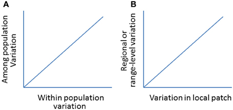
Figure 10. (A) A hypothetic positive relationship between within and among population variations (genetic or morphological; see Oleksiak et al., 2002 for a case study). (B) A hypothetical relationship in population variations (e.g., abundance, distribution) between local- (e.g., patch expansion) and regional- or range-levels (e.g., range expansion).

By examining the changes in local patch sizes in selected locations from year to year, we will be able to relate synchronized patch changes from small (local) to larger (regional) patches and to the whole (global) invaded ranges following climate change (Figure 9). This would allow us to test how reliable to use local patches to predict the changes on larger-scale or the whole invaded range (Figure 10). The basic reasoning behind this idea is that if climate changes similarly across the invaded range, the deviation in the patch dynamics (e.g., area and/or change direction) would indicate the effects of local land use patterns. Otherwise, if the climate becomes warmer (relative to long-term average) in one part of the range but cooler in other parts, we will relate to the causes of the deviations in patch size and shifting direction to local climate changes.

Many aspects mentioned above are being increasingly described, modeled, or visualized using advanced geospatial technologies (such as remote sensing, GPS, GIS, and LiDAR, e.g., Underwood et al., 2003). For example, we can use satellite-based remote sensing technology to make new distribution maps with many other determinant or limiting factors, including details that can better reflect the true structure of species' ranges and species abundance (rather than simply boundary lines). We refine this with remote sensing and modeling analysis to develop maps of current distribution of invasive species in both native and invaded habitats. After assembling and incorporating necessary input information from existing geographic and climatic databases, we will execute the models to predict distribution of the species using current climate and land cover as well as alternative climate and land cover change scenarios.

Sampling

While discrepancies in sampling strategy (e.g., sample size, location, spatial arrangement, and timing) have always been a confounding factor among studies, extensive sampling of major population parameters and vital rates toward all major cardinal directions across species' ranges is clearly needed (Kluth and Bruelheide, 2005; Yakimowski and Eckert, 2007). More importantly, the pivotal role of range shape (geometry), orientation, and structure has often been overlooked or ignored in assessing the C-M changes in genetic diversity. For example, the genetic diversity would be quite different when sampled in different cardinal directions from the center to margin, i.e., among C-N, C-S, C-W, and C-E directions unless the range is very small, not near-circular, or strong environmental clines affect genetic structure. Yet, the patterns in genetic variation measured in different directions cannot be simply averaged to generalize the C-M patterns for the species with a succinct interpretation (e.g., Howes and Lougheed, 2008; see also Garner et al., 2004).

The density of a species is “real” but the way we measure it is “artificial” and can be affected by spatial-temporal resolution or sampling scale (i.e., quadrat or window size) and techniques (MacKenzie et al., 2003). While we all agree that broader surveys across whole species range is needed, systematic sampling that includes quadrats with zero counts within clearly identified range boundaries is a key requirement. This is because density would be overestimated toward margin if selective sampling (i.e., only the patches with the species are sampled) is performed, especially with smaller quadrats. Survey the whole species range might be more revealing although species distribution often show self-similarity (or power-scaling; Hui and McGeoch, 2007) within and across the whole species ranges.

The species ranges are fractal and the way we measure range size is “artificial” and can be affected by spatial-temporal resolution or sampling scale (i.e., frame size, quadrat size, window size) and techniques (Gaston, 2003). The precision of measured distribution increases with decreasing scale. An extreme case would be when sampling is only conducted in the patches where the species is found or the winder size is so small that only covers only one individual (in the latter case, density would be the same across the species range). When all patches (including those with zero individuals) within a species' range are measured and analyzed in total using a range of window sizes (e.g., Fortin et al., 2005), the overall density would still be higher at the range centers. An increase in grid size (observational window size) can increase the chance of overestimating the distribution/occupancy of species thus sometimes fails to detect the abundance centers (Hui and McGeoch, 2007).

Previous samplings are often incomplete or uneven across the species' ranges. The most common approach that has been used so far is conducting paired comparison between core and peripheral populations (dichotomic), often in one direction (that is, the marginal populations are from one cardinal direction only; see review by Eckert et al., 2008). Other paired comparisons include core-core and peripheral-peripheral comparisons. The latter can further be analyzed through comparing neighboring populations and distant populations, i.e., those on the opposite edge of the species' range, especially between N and S populations with latitudinal climate disparities (Figure 2). Because different results would be expected from each of these paired comparisons mentioned above and simple C-M comparisons miss many other processes taking place between C- and M- populations, to make accurate and meaningful comparisons, it is critical to (1) sample entire species ranges when possible, (2) make clear distinctions between the total population and a single population in each ring, and distinctions between population sizes and densities, and (3) distinguish the comparison between pairs of populations, some from the center and others from the margin in one direction only, from the comparisons between selected central and selected marginal populations from different cardinal directions combined (e.g., Howes and Lougheed, 2008). For species with large latitudinal ranges, comparisons between N and S or among all populations along the S-N gradient might reveal stronger genetic diversity patterns than those along the C-M gradients.

Genetic or morphological variation can also be compared among and within populations across a species' range. Despite the reduced genetic variation within individual populations, the greater isolation among marginal populations due to their smaller sizes and greater distances among them would increase the overall variation among marginal populations. This overall greater genetic diversity in all marginal populations has previously been overlooked or underestimated as Figure 3 (top) demonstrates. At the margin where genetic diversity in a single population is relatively low, species spread or range expansion may be enhanced by a number of means such as increased dispersal and gene flow from interior populations. For example, Schmeller et al. (2005) report that, by incorporating locally adapted genes (alleles) from related species through hybridogenesis in marginal populations, range borders of certain species still gain or retain the ability to expand, despite the relative low genetic diversity.

Improved understanding of species range and abundance structure is still so much depending on sampling procedures and technology (Fortin et al., 2005). In nature, individuals of any species are not continuously distributed across its entire ranges, even in the densest populations. Thus, the description of species range is sensitive to spatial scale and timeframes. In most cases, sufficiently small window size (relative to organism body size and dispersability) is needed to capture the meaningful patterns in species distribution. In addition, the fractal nature of land surface makes measuring the distribution area even more difficult (Milne, 1991). For example, the actual surface area will decrease with increasing scale due to lost fractal dimension yet the measured occupation area for a species is likely to increase because no species actually covers all the space in the grid we choose to use (i.e., window size).

Two related issues need to be addressed: (1) when a species range boundary is clearly defined and accurately located, sampling quadrats of same size must be evenly across the whole species range; and (2) if quadrat size is much smaller than the patch size, it is possible that the density at the center of a marginal patch is similar to the margin of a central patch. An extreme case would be when sampling is only conducted in the patches where the species is found or the winder size is so small that only covers only one individual (in the latter case, density would be the same across the species range). When all patches (including those with zero individuals) within a species' range are measured and analyzed in total using a range of window sizes (e.g., Fortin et al., 2005), the overall density would still be higher at the range centers. At both center and margin, if we examine small patches within the entire range of species with “exceptional” abundance curves, the Gussian pattern may be common, although the exact shape may vary from patch to patch (Gaston, 2003).

While extensively monitoring most if not all populations within species' ranges is ideal when ranges are small or resources are not limited, intense monitoring the marginal populations may be more efficient when species ranges are large and resources are limited. All the sampling limitations (above) could be overcome due to the unprecedented advances in molecular and geospatial technologies plus the accumulated knowledge regarding C and M populations. Over large scales such as the whole range level, atlas and herbarium data have also been proved very helpful (Gimona and Brewer, 2006).

Human Activity Alters the Structure of Species Ranges

As major cause of global change, human activities have drastically modified earth's surface. One of the most visible changes would be the great alternation of species ranges through species introduction (both intentional and unintentional). Unlike species introductions that form new centers in remote locations, human land use may cause disruption of originally continuous distribution through habitat fragmentation. The species abundance curves might have changed especially over the regions or landscapes where agriculture or selective harvesting (over size or age; Fenberg and Rivadeneira, 2011) takes place. Such alternation and disruption in species ranges occurs even the underlying environmental variables such as climate might still be altered to a smaller extent. An associated drastic change would be the increasing formation of multiple abundance centers in relatively isolated patches due to the break-ups of formerly a single or a few centers in in natural settings as a consequence of habitat fragmentation and species invasions. These human-induced changes thus modify the original C-M patterns of the same species.

To date, most studies related to global (climate) change have investigated species range shift, especially at margins (limits, or boundaries); and relatively much less effort is devoted to examine how (internal) range structure has changed. The evidence of human destruction of original distribution of native species is abundant, leading to openings for invasive species. Indeed, given the present and projected accelerating degree and extent of human activities, the concepts, ideas, and configuration of (at least some) species ranges studied in Darwin's era (1800 s) might have evolved drastically. For example, the extensive croplands in the Great Plains may have divided original or existing species ranges into smaller pieces by fragmentation and each smaller patch may form a new and smaller abundance center. In such cases, the edge of croplands may not be treated as patch edges for locating abundance center as such edges are artificial and abrupt but the rest (opening) places become available for invasive species. For some others, the patches are still somehow connected through remained patches or corridors such as riparian zones or through windbreaks. In the same region, however, many species (often less common ones) might have formed disjunct distributions because the minimum population size cannot be maintained through highly patchy or fragmented landscapes.

In all these case with growing human influences, the artificially reduced abundance and patch size within species ranges would dramatically alter the features of species abundance centers (size, shape, location) thus describing and explaining abundance patterns (centers) for many native species may no longer be feasible (i.e., they are no longer in “natural” states). At the same time, the abundance curves for invading species may follow the newly created “gaps” where they interact with native species although underlying environmental conditions allow very different curves. In such situations, the study of C-M gradients for invasive species must first consider various forms of species interactions (e.g., competition, predation, and mutualism; With, 2002).

Conservation and Management Implications

When and where, time, resources and manpower allow, simultaneously monitoring as many parameters as possible within and across the whole species range might be the best solution for the management of invasive species. This will help identify the critical factors responsible at different invaded locations. For example, the causes of fast spread of kudzu (Pueraria lobata) in Florida (USA) may be different from that in Ontario (Canada) (Li et al., 2011). Therefore, the applications of research results for control and management of a particular invasive species from one location might not be suitable for other locations across the species' invaded ranges. Also, when we are able to identify the land use patterns that either promote or reduce invasive species invasion, recommendation can then be made accordingly to the landowners and managers to develop optimal land use plans. If we could better predict where invasive species might invade in the future under projected climate change scenarios and land use patterns, early warning and prevention are much more efficient than later management.

Range geometry (as well as latitude in some cases) clearly has significant conservation implications. Simplified C-M models show that the majority of genetic diversity and resources are actually located in populations between the range center and margin (Figure 3). Although marginal populations are usually smaller, more isolated, less stable, and thus more endangered, to a large degree, they rely on central or interior populations as their reliable genetic resources for long-term persistence (Howe et al., 1991). Thus, monitoring or controlling marginal (sink) populations alone is not sufficient as it neglects their genetic “sources” from the range center and those in the middle between center and margin. In light of these recent findings, ideally, management efforts should be allocated to the entire species range whenever possible. The same is true for conservation as shown by McDonald-Madden et al. (2008) who proposed a similar balanced and dynamic conservation strategy asserting that, to be effective, managers should conserve as many populations over space and time as possible (see also Furlow, 1995). The role of range-geometry metrics such as location (i.e., latitude), shape, and orientation in governing spatial genetic diversity distribution must be considered in allocating management efforts.

Although I only consider species with circular or linear ranges as examples, the results clearly demonstrate the effects of range geometry. For species with ranges of special shapes (e.g., linear, truncated, and disjunct) or sizes, the effects of range geometry need to be examined separately and different approaches may be needed. However, in any case, because the range margin covers much more area than the center (Figures 2, 3), it presents a great challenge for effective monitoring the population dynamics across species ranges. For this reason, prioritizing certain marginal populations (e.g., N vs. S) for detailed research and monitoring is needed. On the other hand, if financial and other resources are too limited for certain species with relatively larger ranges, because the equatorial edge of species may hold a unique set of genetic diversity different from either the core or the poleward periphery and because these genotypes have the greatest potential to be lost from the species under climate change (as conditions at the equatorial edge will likely become unsuitable first), a greater number of studies should be comparing the equatorial edge with the core or the entire range and conservation efforts may start from the equatorial edge.

For allocating management efforts on invasive species, perhaps among the most challenging issues is whether central or marginal populations should be given higher priority. Some would argue that central populations should be controlled first because they often hold the high genetic diversity and thus represent the major “sources” of genetic variation, while others suggest giving priorities to marginal populations because they are the “invasion fronts” and may be more sensitive climate change. In native species conservation, marginal populations have so far been the major focus because they (1) are usually more isolated and have low density, and (2) interact more extensively and intensively with resident species. For invasive species management, however, they might be equally important both for understanding what limit the species spread and for developing control measures.

When resources are available, invasive species management should increasingly monitor as many populations across a species' range as possible, rather than giving priorities to certain populations (Burgman et al., 2013). This is mostly because all populations are related to each other (Hanski, 1999), and each one contributes in somewhat unique way to the overall genetic variation. Future studies need to incorporate often-overlooked range geometry and C-M gradients in multi-directions, and to compare C-M patterns in genetic and phenotypic diversity of the same species in both native and exotic regions (Guo, 2006; Molins et al., 2014). Such studies could reveal patterns unseen through simple and paired C-M comparisons and information about limiting factors controlling the species in its native ranges which can be used for developing more effective management methods in invaded ranges.

Challenges and Opportunities

Studies of biotic invasions still face many challenges. In particular, to date most studies related to the C-M models and abundance center hypothesis have not examined whole species ranges, leading to many inconsistent results. When time and resources allow, simultaneously monitoring populations across the whole species' ranges might be the best solution. Where resources are limited, however, an efficient way to determine the limiting factors of species spread would be to use marginal populations and biophysical conditions at the species' range boundary because they are likely most sensitive to environmental change. While the C-M approach may be most effective for species with proximate circular ranges or patches, different approaches may be developed for others to accommodate the specific range geometry (e.g., size and shapes).

Field sampling needs to be carefully designed and conducted at the “right” times in growing season when populations of targeted invasive species show critical stages in life cycle such as germination, flowering, and seed production. In some cases where invasive species show clear elevational gradients in distribution, changes in upper and lower elevational limits could be used to mirror the effects of climate change on northern and southern limits (Figure 8). Investigation of patch boundaries within the geographic range of the species could be very useful for examining the regional effects of pattern and history of land use on entire species' ranges.

New techniques and more comprehensive (and balanced) sampling are needed for better understanding species' abundance and genetic structure across its range. Given the long-term goals in invasive species management, the following objectives related to the C-M gradients under global and regional changes are critical and need immediate attention.

(1) To identify and compare the boundary conditions either limiting or promoting the invasion of exotic species at the six cardinal directions (i.e., horizontally N, S, W, E, and vertically upper/lower limits), such as the climate and soil conditions (e.g., allelopathy; Peng et al., 2004) and disturbance regimes.

(2) To examine the boundary and C-M dynamics and to predict where and at what pace invasive species might further invade under various climate change and land use scenarios (GCMs; Hobbs, 2000; Albright et al., 2010; Bertelsmeier et al., 2013). This is needed for developing early-warning systems/techniques and can be done using simulation techniques (Carpenter et al., 2011).

(3) Use improved modeling and spatial technology to better simulate, predict, and map future invasions under various climatic and land use scenarios based on the invasion/spread history and present contour abundance curves (Albright et al., 2010; Olatinwo et al., 2013; Figure 7).

To reach these goals, the following questions need to be addressed first: (1) whether the genetic structure of selected species may have changed since introduction from native regions (Guo, 2006; Molins et al., 2014), (2) how invasiveness develops at margins through population's evolutionary potential and ability to adapt to changing environments, and (3) what specific genotypes are most invasive and where they are located along the C-M gradients? To answer these questions, we can take several immediate actions, including (1) collecting data to track historical invasion in relation to pathways, climate, and land use, (2) collecting comparable information for comparisons in C-M patterns between populations in both native vs. exotic regions, and (3) conducting experimental research (e.g., translocations, common gardens) to compare populations along the C-M gradients and between native and exotic ranges.

Conclusions

Traditional dichotomic C-M comparisons are simple and easier but often miss critical gradients and processes occurring in C-M continuum. The results from a few paired central-marginal comparisons also depend on the specific location and direction (such as N-S) the marginal population is chosen (Fenberg and Rivadeneira, 2011), thus overshadow the true difference with central populations. This overview stresses the importance of range-wide sampling in all major cardinal directions with the C-M gradients as the main focus that may reveal a more complete picture regarding population structure and dynamics.

Because of the complex nature of the problems involved, a major gap in studies of invasive species is the lack of integration and cooperation among disciplines and across multiple spatiotemporal scales or taxonomic groups (Ricklefs, 2003). With limited resources, one of the most efficient ways is to monitor as many factors as possible at the patch or range borders and across the selected C-M gradients because these locations are most sensitive to environmental changes and are relatively easy to study because they involve small focal areas. The rapidly accruing genetic and filed data from expanded molecular and GIS technologies and sampling efforts would enable us better understand range-wide population dynamics and manage the invasive species more effectively.

Conflict of Interest Statement

The author declares that the research was conducted in the absence of any commercial or financial relationships that could be construed as a potential conflict of interest.

Acknowledgments

I thank M. Taper for stimulating discussions on the subject, T. Albright, J. Falcone, J. Hellmann, D. Lee, D. Oro, A. Ryabov, and J. Wen for helpful comments on earlier versions. This work is partly supported by NSF grants (DEB-0640058 and DEB1241932).

References

Albright, T. P., Chen, H., Chen, L., and Guo, Q. F. (2010). The ecological niche and reciprocal prediction of the disjunct distribution of an invasive species: the example of Ailanthus altissima. Biol. Invas. 12, 2413–2427. doi: 10.1007/s10530-009-9652-8

CrossRef Full Text

Alexander, J. M., and Edwards, P. J. (2010). Limits to the niche and range margins of alien species. Oikos 119, 1377–1386. doi: 10.1111/j.1600-0706.2009.17977.x

CrossRef Full Text

Alleaume-Benharira, M., Pen, I. R., and Ronce, O. (2006). Geographical patterns of adaptation within a species' range: interactions between drift and gene flow. J. Evol. Biol. 19, 203–215. doi: 10.1111/j.1420-9101.2005.00976.x

Pubmed Abstract | Pubmed Full Text | CrossRef Full Text

Angert, A. L. (2006). Demography of central and marginal populations of monkeyflowers (Mimulus cardinalis and M. lewisii). Ecology 87, 2014–2025. doi: 10.1890/0012-9658(2006)87[2014:DOCAMP]2.0.CO;2

Pubmed Abstract | Pubmed Full Text | CrossRef Full Text

Angert, A. L., Bradshaw, H. D. Jr., and Schemske, D. W. (2008). Using experimental evolution to investigate geographic range limits in monkeyflowers. Evolution 62, 2660–2675. doi: 10.1111/j.1558-5646.2008.00471.x

Pubmed Abstract | Pubmed Full Text | CrossRef Full Text

Antonovics, J., Newman, T. J., and Best, B. J. (2001). “Spatially explicit studies on the ecology and genetics of population margins,” in Integrating Ecology and Evolution in a Spatial Context, eds J. Silvertown and J. Antonovics (Oxford: Blackwell), 91–116.

Bahn, V., O'Connor, R. J., and Krohn, W. B. (2006). Effect of dispersal at range edges on the structure of species ranges. Oikos 115, 89–96. doi: 10.1111/j.2006.0030-1299.14825.x

CrossRef Full Text

Bakker, E. G., Stahl, E. A., Toomajian, C., Nordborg, M., Kreitman, M., and Bergelson, J. (2006). Distribution of genetic variation within and among local populations of Arabidopsis thaliana over its species range. Mol. Ecol. 15, 1405–1418. doi: 10.1111/j.1365-294X.2006.02884.x

Pubmed Abstract | Pubmed Full Text | CrossRef Full Text

Belyayev, A., and Raskina, O. (2013). Chromosome evolution in marginal populations of Aegilops speltoides: causes and consequences. Ann. Bot. 111, 531–538. doi: 10.1093/aob/mct023

Pubmed Abstract | Pubmed Full Text | CrossRef Full Text

Bertelsmeier, C., Luque, G. M., and Courchamp, F. (2013). Increase in quantity and quality of suitable areas for invasive species as climate changes. Conserv. Biol. 27, 1458–1467. doi: 10.1111/cobi.12093

Pubmed Abstract | Pubmed Full Text | CrossRef Full Text

Bertocci, I., Araujo, R., Vaselli, S., and Sousa-Pinto, I. (2011). Marginal populations under pressure: spatial and temporal heterogeneity of Ascophyllum nodosum and associated assemblages affected by human trampling in Portugal. Mar. Ecol. Prog. Ser. 439, 73–82. doi: 10.3354/meps09328

CrossRef Full Text

Borgatti, S. P., and Everett, M. G. (1999). Models of core/periphery structures. Soc. Netw. 21, 375–395. doi: 10.1016/S0378-8733(99)00019-2

CrossRef Full Text

Bravo-Monzón, A. E., Ríos-Vásquez, E., Delgado-Lamas, G., and Espinosa-García, F. J. (2014). Chemical diversity among populations of Mikania micrantha: geographic mosaic structure and herbivory. Oecologia 174, 195–203. doi: 10.1007/s00442-013-2748-y

Pubmed Abstract | Pubmed Full Text | CrossRef Full Text

Bridle, J. R., and Vines, T. H. (2007). Limits to evolution at range margins: when and why does adaptation fail? Trends Ecol. Evol. 22, 140–147. doi: 10.1016/j.tree.2006.11.002

Pubmed Abstract | Pubmed Full Text | CrossRef Full Text

Brockmann, D., and Helbing, D. (2013). The hidden geometry of complex, network-driven contagion phenomena. Science 342, 1337–1342. doi: 10.1126/science.1245200

Pubmed Abstract | Pubmed Full Text | CrossRef Full Text

Brown, J. H. (1984). On the relationship between abundance and distribution of species. Am. Nat. 124, 255–279. doi: 10.1086/284267

CrossRef Full Text

Brown, J. H. (1995). Macroecology. Chicago: University of Chicago Press.

Burgman, M. A., McCarthy, M. A., Robinson, A., Hester, S. M., McBride, M. F., Elith, J., et al. (2013). Improving decisions for invasive species management: reformulation and extensions of the Panetta–Lawes eradication graph. Divers. Distrib. 19, 603–607. doi: 10.1111/ddi.12055

CrossRef Full Text

Carpenter, S. R., Cole, J. J., Pace, M. L., Batt, R., Brock, W. A., Cline, T., et al. (2011). Early warnings of regime shifts: a whole-ecosystem experiment. Science 332, 1079–1082. doi: 10.1126/science.1203672

Pubmed Abstract | Pubmed Full Text | CrossRef Full Text

Channell, R., and Lomolino, M. V. (2000). Dynamic biogeography and conservation of endangered species. Nature 403, 84–86. doi: 10.1038/47487

Pubmed Abstract | Pubmed Full Text | CrossRef Full Text

Chao, W. S., Serpe, M., Suttle, J. C., and Jia, Y. (2013). Increase in ACC oxidase levels and activities during paradormancy release of leafy spurge (Euphorbia esula) buds. Planta 238, 205–215. doi: 10.1007/s00425-013-1887-z

Pubmed Abstract | Pubmed Full Text | CrossRef Full Text

Chen, Y. G., and Zhou, Y. X. (2006). Reinterpreting central place networks using ideas from fractals and self-organized criticality. Environ. Plann. B Plann. Design 33, 345–364. doi: 10.1068/b31131

CrossRef Full Text

Colautti, R. I., Eckert, C. G., and Barrett, S. C. (2010). Evolutionary constraints on adaptive evolution during range expansion in an invasive plant. Proc. R. Soc. B Biol. Sci. 277, 1799–1806. doi: 10.1098/rspb.2009.2231

Pubmed Abstract | Pubmed Full Text | CrossRef Full Text

Dawson, M. N., Grosberg, R. K., Stuart, Y. T., and Sanford, E. (2010). Population genetic analysis of a recent range expansion: mechanisms regulating the poleward range limit in the volcano barnacle Tetraclita rubescens. Mol. Ecol. 19, 1585–1605. doi: 10.1111/j.1365-294X.2010.04588.x

CrossRef Full Text

Doak, D. F., and Morris, W. F. (2010). Demographic compensation and tipping points in climate-induced range shifts. Nature 467, 959–962. doi: 10.1038/nature09439

Pubmed Abstract | Pubmed Full Text | CrossRef Full Text

Dunning, J. B., Danielson, B. J., and Pulliam, H. R. (1992). Ecological processes that affect populations in complex landscapes. Oikos 65, 169–175. doi: 10.2307/3544901

CrossRef Full Text

Eckert, C. G., Samis, K. E., and Lougheed, S. C. (2008). Genetic variation across species' geographical ranges: the central-marginal hypothesis and beyond. Mol. Ecol. 17, 1170–1188. doi: 10.1111/j.1365-294X.2007.03659.x

Pubmed Abstract | Pubmed Full Text | CrossRef Full Text

Elton, C. S. (1958). The Ecology of Invasions by Plants and Animals. London: Methuen.

Epperson, B. K. (2007). Plant dispersal, neighbourhood size and isolation by distance. Mol. Ecol. 16, 3854–3865. doi: 10.1111/j.1365-294X.2007.03434.x

Pubmed Abstract | Pubmed Full Text | CrossRef Full Text

Feldhamer, G. A., Lesmeister, D. B., Devine, J. C., and Stetson, D. I. (2012). Golden mice (Ochrotomys nuttalli) co-occurrence with Peromyscus and the abundant-center hypothesis. J. Mamm. 93, 1042–1050. doi: 10.1644/11-MAMM-A-345.2

CrossRef Full Text

Fenberg, P. B., and Rivadeneira, M. M. (2011). Range limits and geographic patterns of abundance of the rocky intertidal owl limpet, Lottia gigantea. J. Biogeogr. 38, 2286–2298. doi: 10.1111/j.1365-2699.2011.02572.x

CrossRef Full Text

Fordham, D. A., Akçakaya, H. R., Araújo, M. B., Keith, D. A., and Brook, B. W. (2013). Tools for integrating range change, extinction risk and climate change information into conservation management. Ecography 36, 956–964. doi: 10.1111/j.1600-0587.2013.00147.x

CrossRef Full Text

Forman, R. T. (1995). Land Mosaics: The Ecology of Landscapes and Regions. Cambridge: Cambridge University Press.

Fortin, M. J., Keitt, T. H., Maurer, B. A., Taper, M. L., Kaufman, D. M., and Blackburn, T. M. (2005). Species' geographic ranges and distributional limits: pattern analysis and statistical issues. Oikos 108, 7–17. doi: 10.1111/j.0030-1299.2005.13146.x

CrossRef Full Text

Frankham, R. (1996). Relationship of genetic variation to population size in wildlife. Biol. Conserv. 10, 1500–1508. doi: 10.1046/j.1523-1739.1996.10061500.x

CrossRef Full Text

Freeman, L. C. (1979). Centrality in social networks: I. Conceptual clarification. Soc. Netw. 1, 215–239. doi: 10.1016/0378-8733(78)90021-7

CrossRef Full Text

Furlow, F. B. (1995). Peripheral populations and range collapse. Conserv. Biol. 9:1345. doi: 10.1046/j.1523-1739.1995.09061345.x

CrossRef Full Text

Garner, T. W., Pearman, B., and Angelone, S. (2004). Genetic diversity across a vertebrate species' range: a test of the central-peripheral hypothesis. Mol. Ecol. 13, 1047–1053. doi: 10.1111/j.1365-294X.2004.02119.x

Pubmed Abstract | Pubmed Full Text | CrossRef Full Text

Gaston, K. J. (2003). The Structure and Dynamics of Geographic Ranges. Oxford: Oxford University Press.

Gimona, A., and Brewer, M. J. (2006). Local environmental effects and spatial effects in macroecological studies using mapped abundance classes: the case of the rook Corvus frugilegus in Scotland. J. Anim. Ecol. 75, 1140–1146. doi: 10.1111/j.1365-2656.2006.01134.x

Pubmed Abstract | Pubmed Full Text | CrossRef Full Text

Gleick, J. (1987). Chaos: Making a New Science. London: Cardinal.

Grant, M. C., and Antonovics, J. (1978). Biology of ecologically marginal populations of Anthoxanthum odoratum. I. phenetics and dynamics. Evolution 32, 822–838. doi: 10.2307/2407497

CrossRef Full Text

Guo, Q. F. (2006). Intercontinental biotic invasions: what can we learn from native populations and habitats? Biol. Invasions 8, 1451–1459. doi: 10.1007/s10530-005-5834-1

CrossRef Full Text

Guo, Q. F. (2012). Incorporating latitudinal and central-marginal trends in assessing genetic variation across species ranges. Mol. Ecol. 21, 5396–5403. doi: 10.1111/mec.12012

Pubmed Abstract | Pubmed Full Text | CrossRef Full Text

Guo, Q. F., Sax, D. F., Qian, H., and Early, R. (2012). Latitudinal shifts of introduced species: possible causes and implications. Biol. Invasions 14, 547–556. doi: 10.1007/s10530-011-0094-8

CrossRef Full Text

Guo, Q. F., Taper, M. L., Schoeneberger, M., and Brandle, J. (2005). Spatial-temporal population dynamics across a species' range: from center to margin. Oikos 108, 47–57. doi: 10.1111/j.0030-1299.2005.13149.x

CrossRef Full Text

Guo, Q., Qian, H., Ricklefs, R. E., and Xi, W. (2006). Distributions of exotic plants in eastern Asia and North America. Ecol. Lett. 9, 827–834. doi: 10.1111/j.1461-0248.2006.00938.x

Pubmed Abstract | Pubmed Full Text | CrossRef Full Text

Hanski, I. (1999). Metapopulation Ecology. Oxford: Oxford University Press.

Hardie, D. C., and Hutchings, J. A. (2010). Evolutionary ecology at the extremes of species' ranges. Environ. Rev. 18, 1–20. doi: 10.1139/A09-014

Pubmed Abstract | Pubmed Full Text | CrossRef Full Text

Harris, L. D. (1988). Edge effects and conservation of biotic diversity. Conserv. Biol. 2, 330–332. doi: 10.1111/j.1523-1739.1988.tb00196.x

CrossRef Full Text

Hengeveld, R. (1989). Dynamics of Biological Invasions. New York, NY: Kluwer.

Hengeveld, R. (1990). Dynamic Biogeography. Cambridge: Cambridge University Press.

Hobbs, R. J. (2000). “Land-use changes and invasions,” in Invasive Species in a Changing World, eds H. A. Mooney and R. J. Hobbs (Washington, DC: Island Press), 55–64.

Holt, R. D., and Keitt, T. H. (2000). Alternative causes for range limits: a metapopulation perspective. Ecol. Lett. 3, 41–47. doi: 10.1046/j.1461-0248.2000.00116.x

CrossRef Full Text

Howe, R. W., Davis, G. J., and Mosca, V. (1991). The demographic significance of ‘sink’ populations. Biol. Conserv. 57, 239–255. doi: 10.1016/0006-3207(91)90071-G

CrossRef Full Text

Howes, B. J., and Lougheed, S. C. (2008). Genetic diversity across the range of a temperate lizard. J. Biogeogr. 35, 1269–1278. doi: 10.1111/j.1365-2699.2007.01867.x

CrossRef Full Text

Hui, C., and McGeoch, M. (2007). Modeling species distributions by breaking the assumption of self−similarity. Oikos 116, 2097–2107. doi: 10.1111/j.2007.0030-1299.16149.x

CrossRef Full Text

Huston, M. A. (2004). Management strategies for plant invasions: manipulating productivity, disturbance, and competition. Divers. Distrib. 10, 167–178. doi: 10.1111/j.1366-9516.2004.00083.x

CrossRef Full Text

Ibrahim, K. M., Nichols, R. A., and Hewitt, G. M. (1996). Spatial patterns of genetic variation generated by different forms of dispersal. Heredity 77, 282–291. doi: 10.1038/hdy.1996.142

CrossRef Full Text

Kawecki, T. J. (2008). Adaptation to marginal habitats. Annu. Rev. Ecol. Evol. Syst. 39, 321–342. doi: 10.1146/annurev.ecolsys.38.091206.095622

CrossRef Full Text

Keitt, T. H., Lewis, M. A., and Holt, R. D. (2001). Allee effects, invasion pinning, and species' borders. Am. Nat. 157, 203–216. doi: 10.1086/318633

Pubmed Abstract | Pubmed Full Text | CrossRef Full Text

Kluth, C., and Bruelheide, H. (2005). Central and peripheral Hornungia petraea populations: patterns and dynamics. J. Ecol. 93, 584–595. doi: 10.1111/j.1365-2745.2005.00997.x

CrossRef Full Text

Kokko, H., and López-Sepulcre, A. (2006). From individual dispersal to species ranges: perspectives for a changing world. Science 313, 789–791. doi: 10.1126/science.1128566

Pubmed Abstract | Pubmed Full Text | CrossRef Full Text

Lammi, A., Siikamäki, P., and Mustajärvi, K. (1999). Genetic diversity, population size, and fitness in central and peripheral populations of a rare plant Lychnis viscaria. Conserv. Biol. 13, 1069–1078. doi: 10.1046/j.1523-1739.1999.98278.x

CrossRef Full Text

Leger, E. A., Espeland, E. K., Merrill, K. R., and Meyer, S. E. (2009). Genetic variation and local adaptation at a cheatgrass (Bromus tectorum) invasion edge in western Nevada. Mol. Ecol. 18, 4366–4379. doi: 10.1111/j.1365-294X.2009.04357.x

Pubmed Abstract | Pubmed Full Text | CrossRef Full Text

Le Roux, J. J., Wieczorek, A. M., and Meyer, J.-Y. (2008). Genetic diversity and structure of the invasive tree Miconia calvescens in Pacific islands. Divers. Distrib. 14, 935–948. doi: 10.1111/j.1472-4642.2008.00504.x

CrossRef Full Text

Lester, S. E., Gaines, S. D., and Kinlan, B. P. (2007). Reproduction on the edge: large-scale patterns of individual performance in a marine invertebrate. Ecology 88, 2229–2239. doi: 10.1890/06-1784.1

Pubmed Abstract | Pubmed Full Text | CrossRef Full Text

Li, Z. Y., Dong, Q., Albright, T. P., and Guo, Q. F. (2011). Natural and human dimensions of a quasi-wild species: the case of kudzu. Biol. Invasions 13, 2167–2179. doi: 10.1007/s10530-011-0042-7

CrossRef Full Text

Liebhold, A., Koenig, W. D., and Bjørnstad, O. N. (2004a). Spatial synchrony in population dynamics. Ann. Rev. Ecol. Evol. Syst. 35, 467–490. doi: 10.1146/annurev.ecolsys.34.011802.132516

CrossRef Full Text

Liebhold, A., Sork, V., Peltonen, M., Koenig, W., Bjørnstad, O. N., Westfall, R., et al. (2004b). Within-population spatial synchrony in mast seeding of North American oaks. Oikos 104, 156–164. doi: 10.1111/j.0030-1299.2004.12722.x

CrossRef Full Text

Lomolino, M. (2001). Elevation gradients of species−density: historical and prospective views. Glob. Ecol. Biogeogr. 10, 3–13. doi: 10.1046/j.1466-822x.2001.00229.x

CrossRef Full Text

MacKenzie, D. I., Nichols, J. D., Hines, J. E., Knutson, M. G., and Franklin, A. B. (2003). Estimating site occupancy, colonization, and local extinction when a species is detected imperfectly. Ecology 84, 2200–2207. doi: 10.1890/02-3090

Pubmed Abstract | Pubmed Full Text | CrossRef Full Text

Maggini, R., Lehmann, A., Kéry, M., Schmid, H., Beniston, M., Jenni, L., et al. (2011). Are Swiss birds tracking climate change? Detecting elevational shifts using response curve shapes. Ecol. Model. 222, 21–32. doi: 10.1016/j.ecolmodel.2010.09.010

CrossRef Full Text

Magurran, A. E. (2007). Species abundance distributions over time. Ecol. Lett. 10, 347–354. doi: 10.1111/j.1461-0248.2007.01024.x

Pubmed Abstract | Pubmed Full Text | CrossRef Full Text

Malchow, H., Petrovskii, S. V., and Venturino, E. (2008). Spatiotemporal Patterns in Ecology and Epidemiology: Theory, Models, and Simulation. London: Chapman and Hall/CRC Press.

Mandak, B., Bímová, K., Plačková, I., Mahelka, V., and Chrtek, J. (2005). Loss of genetic variation in geographically marginal populations of Atriplex tatarica (Chenopodiaceae). Ann. Bot. 96, 901–912. doi: 10.1093/aob/mci242

Pubmed Abstract | Pubmed Full Text | CrossRef Full Text

McDonald-Madden, E., Baxter, P. W. J., and Possingham, H. P. (2008). Subpopulation triage: how to allocate conservation effort among populations. Conserv. Biol. 22, 656–665. doi: 10.1111/j.1523-1739.2008.00918.x

Pubmed Abstract | Pubmed Full Text | CrossRef Full Text

Milne, B. T. (1991). “Lessons from applying fractal models to landscape patterns,” in Quantitative Methods in Landscape Ecology, eds M. G. Turner and R. H. Gardner (New York, NY: Springer), 199–235.

Mistro, D. C., Díaz Rodrigues, L. A., and Petrovskii, S. (2012). Spatiotemporal complexity of biological invasion in a space-and time-discrete predator–prey system with the strong Allee effect. Ecol. Complexity 9, 16–32. doi: 10.1016/j.ecocom.2011.11.004

CrossRef Full Text

Moilanen, A., and Hanski, I. (2001). On the use of connectivity measures in spatial ecology. Oikos 95, 147–151. doi: 10.1034/j.1600-0706.2001.950116.x

CrossRef Full Text

Molins, M. P., Corral, J. M., Aliyu, O. M., Koch, M. A., Betzin, A., Maron, J. L., et al. (2014). Biogeographic variation in genetic variability, apomixis expression and ploidy of St. John's wort (Hypericum perforatum) across its native and introduced range. Ann. Bot. 113, 417–427. doi: 10.1093/aob/mct268

Pubmed Abstract | Pubmed Full Text | CrossRef Full Text

Murphy, H.T., van der Wal, J., and Lovett-Doust, J. (2006). Distribution of abundance across the range in eastern North American trees. Glob. Ecol. Biogeogr. 15, 63–71. doi: 10.1111/j.1466-822X.2006.00194.x

CrossRef Full Text

Nelson, K. E., and Williams, C. M. (2013). Infectious Disease Epidemiology. London: Jones and Bartlett Publishers.

Olatinwo, R., Guo, Q. F., Fei, S. L., Otrosina, W., Klepzig, K., and Streett, D. (2013). “Vulnerability to insects, diseases and invasive plants in relation to climate change,” in Climate Change Adaptation and Mitigation Management Options: A Guide for Natural Resource Managers in Southern Forest Ecosystems, eds J. Vose and K. Klepzig (Boca Raton: CRC Press), 127–172.

Oleksiak, M. F., Churchill, G. A., and Crawford, D. L. (2002). Variation in gene expression within and among natural populations. Nat. Gen. 32, 261–266. doi: 10.1038/ng983

Pubmed Abstract | Pubmed Full Text | CrossRef Full Text

Oro, D. (2013). Grand challenges in population dynamics. Front. Ecol. Evol. 1:2. doi: 10.3389/fevo.2013.00002

CrossRef Full Text

Paetkau, D., Waits, L. P., Clarkson, P. L., Craighead, L., Vyse, E., Ward, R., et al. (1998). Variation in genetic diversity across the range of North American brown bears. Conserv. Biol. 12, 418–429. doi: 10.1046/j.1523-1739.1998.96457.x

CrossRef Full Text

Pease, C. M., Lande, R., and Bull, J. J. (1989). A model of population growth, dispersal and evolution in a changing environment. Ecology 70, 1657-1664. doi: 10.2307/1938100

Pubmed Abstract | Pubmed Full Text | CrossRef Full Text

Peng, S. L., Wen, J., and Guo, Q. F. (2004). Mechanism and active variety of allelochemicals. Acta Bot. Sin. 46, 757–766.

Peterson, A. T., and Vieglais, D. A. (2001). Predicting species invasions using ecological niche modeling: new approaches from bioinformatics attack a pressing problem. Bioscience 51, 363–371. doi: 10.1641/0006-3568(2001)051[0363:PSIUEN]2.0.CO;2

CrossRef Full Text

Petrovskii, S. V., and Li, B. L. (2005). Exactly Solvable Models of Biological Invasion. London: Chapman and Hall/CRC Press.

Pouget, M., Youssef, S., Migliore, J., Juin, M., Médail, F., and Baumel, A. (2013). Phylogeography sheds light on the central–marginal hypothesis in a Mediterranean narrow endemic plant. Ann. Bot. 112, 1409–1420. doi: 10.1093/aob/mct183

Pubmed Abstract | Pubmed Full Text | CrossRef Full Text

Reichert, S. E. (1993). Investigation of potential gene flow limitation of behavioral adaptation in an aridlands spider. Behav. Ecol. Sociobiol. 32, 355–363. doi: 10.1007/BF00183792

CrossRef Full Text

Ricklefs, R. E. (2003). Genetics, evolution, and ecological communities. Ecology 84, 588–591. doi: 10.1890/0012-9658(2003)084[0588:GEAEC]2.0.CO;2

CrossRef Full Text

Ryabov, A. B., and Blasius, B. (2008). Population growth and persistence in a heterogeneous environment: the role of diffusion and advection. Math. Model. Nat. Phenom. 3, 42–86. doi: 10.1051/mmnp:2008064

CrossRef Full Text

Saavedra-Sotelo, N. C., Calderon−Aguilera, L. E., Reyes−Bonilla, H., Paz−García, D. A., et al. (2013). Testing the genetic predictions of a biogeographical model in a dominant endemic Eastern Pacific coral (Porites panamensis) using a genetic seascape approach. Ecol. Evol. 3, 4070–4091. doi: 10.1002/ece3.734

Pubmed Abstract | Pubmed Full Text | CrossRef Full Text

Sagarin, R. D., and Gaines, S. D. (2002). The ‘abundant centre’ distribution: to what extent is it a biogeographical rule? Ecol. Lett. 5, 137–147. doi: 10.1046/j.1461-0248.2002.00297.x

CrossRef Full Text

Samaniego, H., and Marquet, P. A. (2013). Range structure analysis: unveiling the internal structure of species' ranges. Theor. Ecol. 6, 419–426. doi: 10.1007/s12080-013-0177-5

CrossRef Full Text

Samis, K. E., and Eckert, C. G. (2007). Testing the abundant center model using range-wide demographic surveys of two coastal dune plants. Ecology 88, 1747–58. doi: 10.1890/06-1153.1

Pubmed Abstract | Pubmed Full Text | CrossRef Full Text

Schmeller, D. S., Seitz, A., Crivelli, A., and Veith, M. (2005). Crossing species' range borders: interspecies gene exchange mediated by hybridogenesis. Proc. R. Soc. B Biol. Sci. 272, 1625–1631. doi: 10.1098/rspb.2005.3129

Pubmed Abstract | Pubmed Full Text | CrossRef Full Text

Schooley, R. L., and Branch, L. C. (2011). Habitat quality of source patches and connectivity in fragmented landscapes. Biodiver. Conser. 20, 1611–1623. doi: 10.1007/s10531-011-0049-5

Pubmed Abstract | Pubmed Full Text | CrossRef Full Text

Seebens, H., Gastner, M. T., and Blasius, B. (2013). The risk of marine bioinvasion caused by global shipping. Ecol. Lett. 16, 782–790. doi: 10.1111/ele.12111

Pubmed Abstract | Pubmed Full Text | CrossRef Full Text

Shigesada, N., and Kawasaki, K. (1997). Biological Invasions: Theory and Practice. Oxford: Oxford University Press.

Soley-Guardia, M., Radosavljevic, A., Rivera, J. L., and Anderson, R. P. (2014). The effect of spatially marginal localities in modelling species niches and distributions. J. Biogeogr. doi: 10.1111/jbi.12297. (in press).

CrossRef Full Text

Storey Madeoy, J., Strout, J. L., Wurfel, M., Ronald, J., and Akey, J. M. (2007). Gene-expression variation within and among human populations. Am. J. Human Gen. 80, 502–509. doi: 10.1086/512017

Pubmed Abstract | Pubmed Full Text | CrossRef Full Text

Underwood, E., Ustin, S., and DiPietro, D. (2003). Mapping nonnative plants using hyperspectral imagery. Remote Sens. Environ. 86, 150–161. doi: 10.1016/S0034-4257(03)00096-8

CrossRef Full Text

Vallecillo, S., Brotons, L., and Osborne, P. E. (2010). Geographical variation in the distributional constraints along a gradient of population aggregation. Acta Oecol. 36, 666–674. doi: 10.1016/j.actao.2010.10.004

CrossRef Full Text

Veldtman, R., Chown, S. L., and McGeoch, M. A. (2010). Using scale–area curves to quantify the distribution, abundance and range expansion potential of an invasive species. Divers. Distrib. 16, 159–169. doi: 10.1111/j.1472-4642.2009.00632.x

CrossRef Full Text

Wakeley, J. (2004). “Metapopulation genetics,” in Metapopulation biology, eds I. Hanski and O. E. Gaggiotti (San Diego: Academic Press), 175–198.

Watts, M. J., Fordham, D. A., Akcakaya, H. R., Aiello-Lammens, M. E., and Brook, B. W. (2013). Tracking shifting range margins using geographical centroids of metapopulations weighted by population density. Ecol. Model. 269, 61–69. doi: 10.1016/j.ecolmodel.2013.08.010

CrossRef Full Text

Whitham, T. G., Martinsen, G. D., Keim, P., Floate, K. D., Dungey, H. S., and Potts, B. M. (1999). Plant hybrid zones affect biodiversity: tools for a genetic-based understanding of community structure. Ecology 80, 416–428. doi: 10.1890/0012-9658(1999)080[0416:PHZABT]2.0.CO;2

CrossRef Full Text

Whittaker, J. B. (1971). Population changes in Neophilaenus lineatus (L.) (Homoptera: Cercopidae) in different parts of its range. J. Anim. Ecol. 40, 425–443. doi: 10.2307/3253

CrossRef Full Text

Williams, C. K., Ives, A. R., and Applegate, R. D. (2003). Population dynamics across geographical ranges: time-series analyses of three small game species. Ecology 84, 2654–2667. doi: 10.1890/03-0038

CrossRef Full Text

Williamson, M. (1996). Biological Invasions. New York, NY: Springer.

With, K. (2002). The landscape ecology of invasive spread. Conserv. Biol. 16, 1192–1203. doi: 10.1046/j.1523-1739.2002.01064.x

CrossRef Full Text

Wu, J., and Loucks, O. L. (1995). From balance of nature to hierarchical patch dynamics: a paradigm shift in ecology. Q. Rev. Biol. 70, 439–466. doi: 10.1086/419172

CrossRef Full Text

Yakimowski, S. B., and Eckert, C. G. (2007). Threatened peripheral populations in context: geographical variation in population frequency and size and sexual reproduction in a clonal woody shrub. Conserv. Biol. 21, 811–822. doi: 10.1111/j.1523-1739.2007.00684.x

Pubmed Abstract | Pubmed Full Text | CrossRef Full Text

Yin, Z. Y., Peng, S. L., Ren, H., Guo, Q., and Chen, Z. H. (2005). LogCauchy, log-sech and lognormal distributions of species abundances in forest communities. Ecol. Model. 184, 329–340. doi: 10.1016/j.ecolmodel.2004.10.011

CrossRef Full Text