Dissecting genetic effects with imprinting

Introduction

Classical models of genetic effects were established almost one century ago for assembling biometric observations with Mendelian genetics (Fisher, 1918; Provine, 1971). This way, mechanistic explanations were provided for interesting properties of quantitative traits that had been revealed in the nineteenth century, particularly the regression toward mediocrity (Galton, 1886). A key concept in this theory is the split of effects of allele substitutions into additive and non-additive components, since the population variance of the additive components was shown to determine the resemblance between relatives within that population (see e.g. Falconer and Mackay, 1996).

The practicality of that rule keeps on being of huge importance nowadays. By assessing the resemblance between relatives for a trait within one generation of a population (which requires tracking relatedness and phenotype scores) it is possible to estimate the additive variance of that trait at that population. That estimate may in its turn be used to predict the resemblance between parents and their offspring and hence the response to selection in the forthcoming generation. Thus, although the theory behind relies on genetic effects, no direct information about the genes underlying a trait in a population is necessary in practice for estimating parameters with convenient predictive power.

With time, molecular, statistical and computational tools have enabled mapping experiments to be performed even in non-model species (see e.g. Rifkin, 2012). The need to update models of genetic effects for making the most of this new source of information was soon pointed out (Cheverud and Routman, 1995), leading to the development of models of genetic effects depicting the GP map as effects of allele substitutions from individual genotypes (Hansen and Wagner, 2001). This is the context in which the Natural and Orthogonal Interactions (NOIA) model of genetic effects was developed (Álvarez-Castro and Carlborg, 2007; Álvarez-Castro and Yang, 2011).

NOIA is a generalization of models of genetic effects that unifies the individual-based formulations mentioned right above with the aforementioned classical approaches, which depict the GP map in terms of effects of allele substitutions averaged over populations. As an example, this approach has enabled analyses of the role of epistatic interactions during the artificial selection process leading to the domestication of chicken (Álvarez-Castro et al., 2008). The classical population-referenced models are convenient for obtaining genetic effects of growth rate from the data generated in quantitative trait loci (QTL) experiments. But, next, those have to be transformed into individual-based genetic effects for analyzing how allele substitutions could have occurred in genes underlying growth rate from the reference of the genotype of the wild ancestors of current domestic chicken. In general, being able to transform between the individual- and the population-referenced approaches opens new opportunities of analyses of gene effects and interactions, as reviewed by Álvarez-Castro (2012).

QTL analyses eventually focussed also on the quest for imprinted genes and the estimation of imprinting effects (Knott et al., 1998). The traditional scheme of either maternal or paternal allele-effect silencing is known not to be universal—the callypige phenotype in sheep being a remarkable counterexample for this (Cockett et al., 1996). Indeed, several alternative patterns of imprinting have been described more recently (e.g. Wolf et al., 2008; Xiao et al., 2013). In general, a gene is imprinted for a trait when heterozygotes with different parent-of-origin of their alleles are associated to different phenotypes. Hence, imprinting always involves some kind of dominance (since at least one of the two cases will depart from the mid-homozygote expectation).

New models of genetic effects, involving also epistasis, have recently been proposed to detect and analyze imprinted genes (Wolf and Cheverud, 2009). Here, the discussion on how to model genetic effects in the presence of imprinting is resumed with emphasis on the conceptualization (and thus the biological meaning) of all genetic effects involved. Two different options of extending NOIA to imprinting are developed and pondered in order to stress that the meaning of the genetic effects with imprinting must be considered with particular caution.

Individual- and Population-Referenced Genetic Effects

First, let us recall the most basic expressions and facts of NOIA (from Álvarez-Castro and Carlborg, 2007; Álvarez-Castro et al., 2012). The effects of allele substitutions can be expressed in terms of additive (a) and dominance (d) effects in matrix notation as G = SE, which, for one non-imprinted locus with two alleles (A₁, A₂) and using the homozygote for the first allele as reference, expands to:

$\begin{array}{cc}\left(\begin{array}{c}{G}_{11}\\ G_{12}\\ G_{22}\end{array}\right)=\left(\begin{array}{ccc}1& 0& 0\\ 1& 1& 1\\ 1& 2& 0\end{array}\right)\left(\begin{array}{c}R\\ a\\ d\end{array}\right)& \left(1\right)\end{array}$

In this expression, E is the vector of genetic effects (including also the reference point R), G is the vector of genotypic values (accounting for the expected phenotype for each of the genotypes), and S is the genetic-effect design matrix, which determines how the genetic effects are defined as a reparameterization of the genotypic values. This point is easier to visualize through the equivalent expression E = S⁻¹ G:

$\begin{array}{cc}\left(\begin{array}{c}R\\ a\\ d\end{array}\right)=\left(\begin{array}{ccc}1& 0& 0\\ -\raisebox{1ex}{$1$}\!\left/ \!\raisebox{-1ex}{$2$}\right.& 0& \raisebox{1ex}{$1$}\!\left/ \!\raisebox{-1ex}{$2$}\right.\\ -\raisebox{1ex}{$1$}\!\left/ \!\raisebox{-1ex}{$2$}\right.& 1& -\raisebox{1ex}{$1$}\!\left/ \!\raisebox{-1ex}{$2$}\right.\end{array}\right)\left(\begin{array}{c}{G}_{11}\\ G_{12}\\ G_{22}\end{array}\right)& \left(2\right)\end{array}$

Since a = (G₂₂ − G₁₁)/2 is half the distance between the genotypic values of the two homozigotes, adding two additive effects from the genotypic value of the reference genotype A₁A₁ (G₁₁) brings us to the genotypic value of the other homozygote (G₂₂). Thus, adding one only additive effect brings us to the midpoint between the two homozygotes, from which further adding the dominance effect brings us to the genotypic value of the heterozygote (G₁₂). Indeed, the dominance effect d = G₁₂ − (G₁₁ + G₂₂)/2 measures the deviation of the heterozygote from its additive expectation.

More general expressions, enabling the use of any genotype as reference point, have been developed. In any case, the split of effects of allele substitutions from the reference of an individual genotype into additive and interaction components has direct evolutionary meaning. Indeed, assuming that the genotypic values reflect fitness, a quick comparison of the additive and dominance effects provides the equilibrium properties of the system (either one stable or one unstable polymorphic equilibrium, or fixation of a particular allele, which may occur asymptotically with complete dominance). For the simple case of one locus with two alleles, this information can also be retrieved visually from the representation of the raw genotypic values—the genetic effects become more useful for systems of increasing complexity.

On the other hand, the classical additive and interaction population-referenced genetic effects are useful for analyzing properties of particular populations, with given genotype frequencies (p_ij, with p_i = p_ii + 1/2 p₁₂ being the allele frequencies and μ the phenotype mean). They are average effects of allele substitutions over populations and they can be obtained by a regression of the genotypic values on the allele content. The general expression for two alleles can be written as:

$\begin{array}{cc}\left(\begin{array}{c}{G}_{11}\\ G_{12}\\ G_{22}\end{array}\right)=\left(\begin{array}{ccc}1& -2p_2& -\frac{p_{12}{p}_{22}}{2p_1{p}_2-\raisebox{1ex}{$1$}\!\left/ \!\raisebox{-1ex}{$2$}\right.p_{12}}\\ 1& p_1-p_2& \frac{p_{11}{p}_{22}}{p_1{p}_2-\raisebox{1ex}{$1$}\!\left/ \!\raisebox{-1ex}{$4$}\right.p_{12}}\\ 1& 2p_1& -\frac{p_{11}{p}_{12}}{2p_1{p}_2-\raisebox{1ex}{$1$}\!\left/ \!\raisebox{-1ex}{$2$}\right.p_{12}}\end{array}\right)\left(\begin{array}{c}\mu \\ \alpha \\ \delta \end{array}\right)& \left(3\right)\end{array}$

The parameters of this model are summarized in Table 1. The link between expression (3) and the previous ones comes easy, by just taking into account that the genotypic values remain the same. From any two expressions of this kind, G = S₁E₁ and G = S₂E₂, the genetic effects can be transformed into each other directly as:

$\begin{array}{cc}{E}_2={(S_2)}^{-1}{S}_1{E}_1& \left(4\right)\end{array}$

TABLE 1

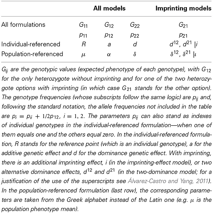
Table 1. Summary of the parameters of the models in this article.

Interactions Make a Difference

Using expression (4), it is easy to derive that a GP map in which d = 0 fulfills δ = 0 and α = a, regardless of the genotypic frequencies. However, the presence of interactions makes the relationship between individual- and population-referenced genetic effects to be far from trivial—and, indeed, far more interesting (Álvarez-Castro and Le Rouzic, 2014). This is illustrated by two simple examples in Figure 1. These graphs show the linear regression (solid line) of the genotypic values (discs) on the allele content (horizontal axis) for a particular population (with specific allele frequencies), as well as the decomposition of the genetic variance (curves) for any allele frequencies.

FIGURE 1

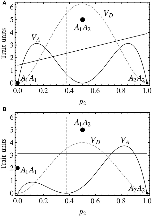
Figure 1. Genotypic values (discs) and variance decomposition (curves) of one-locus, two-allele (A₁ and A₂), non-imprinted genetic systems with overdominance assuming Hardy–Weinberg proportions for all possible allele frequencies (represented by the frequency of A₂, p₂). The variances (black solid curve for additive, gray dashed curve for dominance) are actually plotted as trait units squared. The size of the discs marking the genotypic values are scaled according to p₁ = 0.625 (approximately, p₁₁ = 0.14, p₁₂ = 0.47, p₂₂ = 0.39). (A) The genotypic values are G₁₁ = 0, G₁₂ = 5, G₂₂ = 0, leading to individual-referenced genetic effects (from the reference of A₁A₁) a = 0, d = 5. At p₂ = 0.375 (p₁ = 0.625, marked by the vertical dashed line), the regression of the genotypic values on the proportional allele content (solid line) is an increasing function with slope (and thus population-referenced additive effect) α = 2.5, indicating that p₂ would increase under directional selection (toward the equilibrium point, p₁ = p₂ = 0.5). (B) The genotypic values are the same as in (A) but for G₁₁ = 2, leading to individual referenced genetic effects of a = −1, d = 4. At p₂ = 0.375 (p₁ = 0.625, marked by the vertical dashed line), the regression of the genotypic values on the proportional allele content (solid line) has α = 0 slope, indicating a polymorphic equilibrium point.

The first example (Figure 1A) shows a case in which the individual-referenced additive genetic effect is nil (the genotypic values of the homozygotes are equal) whereas the dominance effect is not (the genotypic value of the heterozygote is different from them). The slope of the weighted regression of the genotypic values on the allele content provides the population-referenced additive genetic effect, α. In that figure, such regression is shown for a Hardy–Weinberg population with p₁ = 0.625, marked with a vertical dashed line. Since the slope of the regression is positive, so it is α. The second example (Figure 1B) still shows a case of overdominance (the genotypic values of the homozygotes are lower than the one of the heterozygote, i.e., d > |a|), although in this case the individual-referenced additive effect is not nil. However, the regression at p₁ = 0.625 has a slope of zero, indicating that this is a (polymorphic) equilibrium point.

In the context of a population, the decomposition of the genotypic values into additive and interaction effects has its parallel at the level of variances. Indeed, in the second example (Figure 1B), the additive variance is nil at p₁ = 0.625. Coming back to the first example (Figure 1A), the additive variance is not nil at p₁ = 0.625 (where the regression slope is not either nil) and, more in general, the additive variance, which determines the selection response, dominates the extremes of the graph (40% of the possible frequencies), indicating very efficient selection response of those populations (toward the equilibrium point, with p₁ = 0.5, where the additive variance is nil).

Thus, throughout these examples it becomes evident that interaction makes it possible both to have nil individual-referenced with non-nil population-referenced additive effects and vice versa. Overall, the presence of interactions unveils that individual- and population-referenced genetic effects have different meanings. The later ones reflect properties of populations (the additive effect and the additive variance are nil at equilibrium frequencies) whereas the former ones are effects of allele substitutions from individual references (the additive effect is nil when the homozygotes have equal genotypic values). Keeping this in mind aids interpretation of the subsequent developments and discussion.

Modeling Imprinting: How Many Additive and Dominance Effects?

When considering one imprinted locus with two alleles, we could be tempted to try to fit it into a one-locus four-allele genetic model, since each of the two alleles (with different nucleotide sequences) may be expressed at the level of the phenotype in two ways (each has two possible methylation stages), thus leading to a total of four variants with potentially different effects on the phenotype. One evident issue coming from this scheme arises when considering how segregation is assumed in a one-locus four-allele model, which does not at all consider transformations of the variants into one another through generations (as it is the case of alleles in imprinted genes). Moreover, even if we dismissed any analyses involving segregation, we could not possibly use the multiallelic model for depicting the differences between phenotypes due to allelic variants, as explained below.

Let the two alleles be A₁ and A₂, just as in the cases without imprinting above. Due to imprinting there now also exist the modified variants Ā₁ and Ā₂, summing up to a total of four variants as mentioned just above. In a four-allele model of genetic effects, there are six additive effects, three of which can be retrieved from the other three (see e.g. Álvarez-Castro and Yang, 2011). These parameters account for effects of allele substitutions between any possible pair of homozygotes, which in our case would be A₁A₁, A₂A₂, Ā₁Ā₁, and Ā₂Ā₂. However, none of these genotypes will be present in any of the individuals of our analyses. More to the point, we cannot easily think of those genotypes as putative artificial constructs, since imprinted loci preclude viability under unbalanced dosages of modified alleles (Kono et al., 2004; Kawahara et al., 2007).

Indeed, the two “homozygotes” of our imprinted biallelic locus actually are A₁Ā₁ and A₂Ā₂—they are allele-wise homozygotes, although not variant-wise homozygotes. Only substitutions implying the pairs A₁-A₂ and Ā₁-Ā₂ are allowed. Thus, one only additive effect of allele substitutions makes sense in this genetic system, involving substitutions of alleles A₁ and A₂ in each of their variants. In the context of the individual-referenced framework, that effect can be measured in a way analogous to the non-imprinted loci as a = (G₂₂ − G₁₁)/2, just considering that with imprinting the “homozygotes” bear two differently modified allelic variants.

Thus, although properly conceptualizing the additive effects of an imprinted locus may require some reflection, they in the end can be modeled in a way that brings no additional complexity as compared to modeling the non-imprinted case. It is the modeling of the dominance effects that will make the difference. It has been discussed just above that from genotype A₁Ā₁ there is one only way of performing two allele substitutions, which leads to genotype A₂Ā₂. There are however two possible ways of performing one only allele substitution from that genotype, leading to either A₁Ā₂ or A₂Ā₁. Consequently, considering two possible dominance effects (one for each parent-of-origin of the two alleles in the heterozygote) emerges as a sensible solution.

To begin with the development of this two-dominance setting, an expression of the genotypic values as a sum of genetic effects of allele substitutions from one reference genotype is firstly provided—as it was done in expression (1) above for a non-imprinted locus. This way (following the same logic as in Álvarez-Castro and Carlborg, 2007; Álvarez-Castro and Yang, 2011), the expression of NOIA from the reference of homozygote A₁Ā₁ can be obtained as:

$\begin{array}{cc}\left(\begin{array}{c}{G}_{11}\\ G_{12}\\ G_{21}\\ G_{22}\end{array}\right)=\left(\begin{array}{cccc}1& 0& 0& 0\\ 1& 1& 1& 0\\ 1& 1& 0& 1\\ 1& 2& 0& 0\end{array}\right)\left(\begin{array}{c}R\\ a\\ d^{12}\\ d^{21}\end{array}\right)& \left(5\right)\end{array}$

All parameters are summarized in Table 1. The genotypic value of A₂Ā₂ is here expressed as the sum of two additive effects from the reference whilst the genotypic values of the heterozygotes involve one additive plus one dominance effect each. The difference between (5) and (1) is that in (5) each heterozygote involves a different dominance effect. By equating the vector of genetic effects in (5) we obtain an extension of expression (2) to imprinting, providing how each of the genetic effects is defined in terms of the genotypic values:

$\begin{array}{cc}\left(\begin{array}{c}R\\ a\\ d^{12}\\ d^{21}\end{array}\right)=\left(\begin{array}{cccc}1& 0& 0& 0\\ -\raisebox{1ex}{$1$}\!\left/ \!\raisebox{-1ex}{$2$}\right.& 0& 0& \raisebox{1ex}{$1$}\!\left/ \!\raisebox{-1ex}{$2$}\right.\\ -\raisebox{1ex}{$1$}\!\left/ \!\raisebox{-1ex}{$2$}\right.& 1& 0& -\raisebox{1ex}{$1$}\!\left/ \!\raisebox{-1ex}{$2$}\right.\\ -\raisebox{1ex}{$1$}\!\left/ \!\raisebox{-1ex}{$2$}\right.& 0& 1& -\raisebox{1ex}{$1$}\!\left/ \!\raisebox{-1ex}{$2$}\right.\end{array}\right)\left(\begin{array}{c}{G}_{11}\\ G_{12}\\ G_{21}\\ G_{22}\end{array}\right)& \left(6\right)\end{array}$

Thus, for instance, the second dominance effect is defined as d²¹ = G₂₁−½(G₁₁ + G₂₂). Expression (6) also entails the general individual-referenced formulation of NOIA for one biallelic imprinted locus, by just replacing the first row of the matrix by (p₁₁, p₁₂, p₂₁, p₂₂), so that any genotype may be chosen as reference (e.g. A₂Ā₂ is the reference when p₂₂ = 1 and the remaining p_ij = 0).

For describing the potential response of the imprinted genetic system to one-generation step of selection, a population-referenced formulation [as expression (3) for a non-imprinted locus] is required. Following the same approach as by Álvarez-Castro and Carlborg (2007, Appendix C; see Supplementary Material), such expression can be obtained as:

$\begin{array}{cc}\left(\begin{array}{c}{G}_{11}\\ G_{12}\\ G_{21}\\ G_{22}\end{array}\right)=\left(\begin{array}{cccc}1& -2p_2& -\frac{p_{12}{p}_{22}}{p_{11}{p}_2+p_1{p}_{22}}& -\frac{p_{21}{p}_{22}}{p_{11}{p}_2+p_1{p}_{22}}\\ 1& p_1-p_2& \frac{4p_{11}{p}_{22}+p_{21}(p_{11}+p_{22})}{2(p_{11}{p}_2+p_1{p}_{22})}& -\frac{p_{21}(p_{11}+p_{22})}{2(p_{11}{p}_2+p_1{p}_{22})}\\ 1& p_1-p_2& -\frac{p_{12}(p_{11}+p_{22})}{2(p_{11}{p}_2+p_1{p}_{22})}& \frac{4p_{11}{p}_{22}+p_{12}(p_{11}+p_{22})}{2(p_{11}{p}_2+p_1{p}_{22})}\\ 1& 2p_1& -\frac{p_{11}{p}_{12}}{p_{11}{p}_2+p_1{p}_{22}}& -\frac{p_{11}{p}_{21}}{p_{11}{p}_2+p_1{p}_{22}}\end{array}\right)\left(\begin{array}{c}\mu \\ \alpha \\ {\delta }^{12}\\ {\delta }^{21}\end{array}\right)& \left(7\right)\end{array}$

Using the procedure for inspecting orthogonality of models of genetic effects, also conveyed by Álvarez-Castro and Carlborg (2007, Appendix C; see the Supplementary material), it follows that expression (7) entails an orthogonal decomposition of the genotypic values into additive and dominance components, thus leading to an orthogonal decomposition of the genetic variance. The two dominance effects are however not orthogonal to each other. Overall, it is possible to model a biallelic imprinted locus using one additive and two dominance genetic effects, which makes it straightforward to keep track of the biological meaning of the parameters, in analogy with the non-imprinted case.

Imprinting as a Genetic Effect

The previous setting can be used for detecting imprinting by just developing a procedure for testing whether the two dominance effects are significantly different. To this aim, it seems however more convenient to design a model in which a parameter accounts for the difference between the two heterozygotes, thus leading to a more direct test for imprinting—consisting in just checking whether that parameter is significantly different from zero. Actually, this is in general terms the approach commonly chosen to model imprinting (see e.g. Wolf et al., 2008). Hereafter, NOIA is extended following that approach and thus implemented with a parameter to account for the putative difference between the heterozygotes with different parent-of-origin. As in the previous section, an expression of effects of allele substitutions from the reference of homozygote A₁Ā₁ is here provided in the first place, as:

$\begin{array}{cc}\left(\begin{array}{c}{G}_{11}\\ G_{12}\\ G_{21}\\ G_{22}\end{array}\right)=\left(\begin{array}{cccc}1& 0& 0& 0\\ 1& 1& 1& -1\\ 1& 1& 1& 1\\ 1& 2& 0& 0\end{array}\right)\left(\begin{array}{c}R\\ a\\ d\\ i\end{array}\right)& \left(8\right)\end{array}$

This model is designed for using the midpoint between the two heterozygotes to define the dominance effect and the deviations of the two heterozygotes from that point as the imprinting effect. A graphical comparison explaining how the three models shown in this article (the non-imprinted model, the two-dominances model and the imprinting-effect model) decompose the genotypic values is shown in Figure 2. By equating the vector of genetic effects in (8) it follows:

$\begin{array}{cc}\left(\begin{array}{c}R\\ a\\ d\\ i\end{array}\right)=\left(\begin{array}{cccc}1& 0& 0& 0\\ -\raisebox{1ex}{$1$}\!\left/ \!\raisebox{-1ex}{$2$}\right.& 0& 0& \raisebox{1ex}{$1$}\!\left/ \!\raisebox{-1ex}{$2$}\right.\\ -\raisebox{1ex}{$1$}\!\left/ \!\raisebox{-1ex}{$2$}\right.& \raisebox{1ex}{$1$}\!\left/ \!\raisebox{-1ex}{$2$}\right.& \raisebox{1ex}{$1$}\!\left/ \!\raisebox{-1ex}{$2$}\right.& -\raisebox{1ex}{$1$}\!\left/ \!\raisebox{-1ex}{$2$}\right.\\ 0& -\raisebox{1ex}{$1$}\!\left/ \!\raisebox{-1ex}{$2$}\right.& -\raisebox{1ex}{$1$}\!\left/ \!\raisebox{-1ex}{$2$}\right.& 0\end{array}\right)\left(\begin{array}{c}{G}_{11}\\ G_{12}\\ G_{21}\\ G_{22}\end{array}\right)& \left(9\right)\end{array}$

FIGURE 2

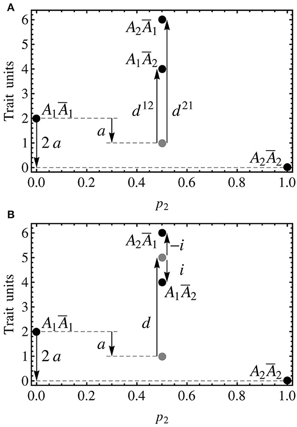
Figure 2. Individual-referenced genetic effects proposed in the text for a one-locus, two-allele, imprinted genetic system. As in the previous figure, the alleles are A₁ and A₂, with the variants due to imprinting being Ā₁ and Ā₂. Although no population frequencies are considered in this figure, the notation of the axes is kept consistent with the other figures, with p₂ = 0.5 indicating the heterozygotes. Also the genotypic values (black discs) are mostly kept, with the one of the heterozygote of Figure 1 (A₁A₂, G₁₂ = 5) being the midpoint between the ones of the two heterozygotes in this figure (A₁Ā₂ and A₂Ā₁, G₁₂ = 4 and G₂₁ = 6, respectively). (A) The two-dominances model is a natural extension of the non-imprinted case that consists in introducing two dominance parameters, one for each heterozygote. As well as in the non-imprinted case, the dominance effects measure departures of the heterozygotes from their additive expectation (gray disc). (B) The imprinting-effect model keeps one only dominance effect that accounts for the departure of the midpoint between the two heterozygotes (upper gray disc) and the midpoint between the homozygotes (lower gray disc), and adds up an imprinting effect for accounting for the distance between the heterozygotes and their midpoint (upper gray disc). Thus, the dominance effect in this model coincides with that of a non-imprinted model (i.e., the one that would be obtained if imprinting was just disregarded).

From this expression it immediately follows that indeed d = ½(G₁₂ + G₂₁) − ½(G₁₁ + G₂₂) (i.e., the dominance effect measures the distance of the midpoint between the two heterozygotes and the additive expectation) and i = ½(G₂₁ − G₁₂) (i.e., the imprinting effect measures the distance of the heterozygotes from the midpoint between them). Expression (9) provides a general individual-referenced formulation, analogously to (6) for the two-dominances model in the previous section. Also in an analogous way as in that section, an orthogonal population-referenced formulation of the imprinting-effect model can be obtained as:

$\begin{array}{cc}\left(\begin{array}{c}{G}_{11}\\ G_{12}\\ G_{21}\\ G_{22}\end{array}\right)=\left(\begin{array}{cccc}1& -2p_2& -\frac{p_{22}\left(p_{12}+p_{21}\right)}{2p_1{p}_2-\raisebox{1ex}{$1$}\!\left/ \!\raisebox{-1ex}{$2$}\right.\left(p_{12}+p_{21}\right)}& 0\\ 1& p_1-p_2& \frac{p_{11}{p}_{22}}{p_1{p}_2-\raisebox{1ex}{$1$}\!\left/ \!\raisebox{-1ex}{$2$}\right.\left(p_{12}+p_{21}\right)}& \frac{-2p_{21}}{p_{12}+p_{21}}\\ 1& p_1-p_2& \frac{p_{11}{p}_{22}}{p_1{p}_2-\raisebox{1ex}{$1$}\!\left/ \!\raisebox{-1ex}{$2$}\right.\left(p_{12}+p_{21}\right)}& \frac{2p_{12}}{p_{12}+p_{21}}\\ 1& 2p_1& -\frac{p_{11}\left(p_{12}+p_{21}\right)}{2p_1{p}_2-\raisebox{1ex}{$1$}\!\left/ \!\raisebox{-1ex}{$2$}\right.\left(p_{12}+p_{21}\right)}& 0\end{array}\right)\left(\begin{array}{c}\mu \\ \alpha \\ \delta \\ \iota \end{array}\right)& \left(10\right)\end{array}$

In this case, the three genetic (additive, dominance and imprinting) effects are fully orthogonal. The independence of the parameters makes this expression to resemble expression (3). Indeed, the decomposition of the genotypic values of the homozygotes into additive and dominance effects in (3) holds in (10), since p₁₂ in (3) is equivalent to (p₁₂ + p₂₁) in (10). Concerning the heterozygotes, in the imprinted case we have two instead of one, leading to an extra row in the genetic-effects design matrix in (10), and there is an extra (imprinting) term in the decomposition, coming from the fourth column of that matrix. That term actually makes the only difference of the decomposition of the genetic effects of the heterozygotes as compared with the decomposition of the heterozygote in the non-imprinted case (3).

Variance Decomposition with Imprinting

The previous expressions and arguments can be extended to the decomposition of the genetic variance with an imprinting variance component, which can easily be obtained from the model in matrix notation above (10) by following the formulae provided by Álvarez-Castro and Yang (2011). In expressions (12) and (13) of that article, the additive and the dominance variance have been obtained as V_A = P^T_G (α_G ○ α_G) and V_D = P^T_G (δ_G ○ δ_G), respectively. In an analogous way (by means of analogous intermediate definitions; see Supplementary Material), a general expression for the imprinting variance can be provided simply as:

$\begin{array}{cc}{V}_O=P_G^{\text{T}}\left({\iota }_G°{\iota }_G\right)& \left(11\right)\end{array}$

Since V_I traditionally stands for the epistatic variance, the subscript O is here chosen for the imprinting variance, ultimately coming from a differential effect of the alleles depending on their parent-of-origin. In any case, it is also possible to obtain the decomposition of the genetic variance by getting all three variance components at the same time, by just following expressions (14) and (15) in Álvarez-Castro and Yang (2011). Indeed, the imprinting variance component emerges from that formulae as a new term due to feeding them with expression (10).

By obtaining the variance decomposition in any of the ways described above (each individually or all simultaneously), it is easy to check that the additive and the dominance variances actually remain the same as for a non-imprinted biallelic locus. Assuming for simplicity the Hardy–Weinberg proportions, they are V_A = 2p₁p₂[a + d (p₁ − p₂)]², V_D = (2dp₁p₂)² (see e.g. Falconer and Mackay, 1996)—, whilst the imprinting variance component can be expressed simply as:

$\begin{array}{cc}{V}_O=2i^2{p}_1{p}_2& \left(12\right)\end{array}$

Figure 3 shows the decomposition of the genetic variance for two cases of imprinting. The genotypic values in Figure 3A are the same as in Figure 2, and thus they also fit the non-imprinted case in Figure 1B, in which the genotypic value of the heterozygote (A₁A₂, G₁₂ = 5) is the midpoint between the genotypic values of the two heterozygotes in Figure 3A (A₁Ā₂ and A₂Ā₁, G₁₂ = 4 and G₂₁ = 6, respectively). Therefore, the additive effects coincide in both cases and the dominance value of the imprinting-effect model in Figure 3A coincides with the simpler non-imprinted model in Figure 1B. Hence, the additive and the dominance variances coincide in both graphs. In Figure 3A there is, though, an extra (imprinting) term of the genetic variance decomposition.

FIGURE 3

Figure 3. Genotypic values (discs) and variance decomposition (curves) of one-locus, two-allele, imprinted genetic systems assuming Hardy–Weinberg proportions. The notation is in accordance with the previous figures (with the addition of a black dashed curve for the imprinting variance). (A) The genotypic values are G₁₁ = 2, G₁₂ = 4, G₂₁ = 6, G₂₂ = 0, leading to individual-referenced genetic effects (from the reference of A₁Ā₁) a = −1, d = 4, i = −1. Since the additive and the dominance effects are the same as in Figure 1B, the additive and the dominance variances coincide and the equilibrium point also remains at p₂ = 0.375. (B) The genotypic values are the same as in (A) but for G₂₁ = 1 (at the midpoint between the two homozygotes), leading to individual referenced genetic effects of a = −1, d = 2.5, i = −2.5. The equilibrium point occurs here at p₂ = 0.3.

As it is the case for dominance, the imprinting variance is higher for intermediate frequencies. In Figure 3A, the relatively small imprinting effect (relatively short distance between the two heterozygotes) leads to a small imprinting variance for all allele frequencies. In Figure 3B, however, it is shown that with larger differences between the two heterozygotes the imprinting variance may dominate the variance decomposition at almost any allele frequencies. And this actually occurs in practice, since this case fits to the callypige pattern mentioned above (with equal or similar phenotype values of the two homozygotes and one of the heterozygotes, relative to a higher value of the remaining heterozygote). Imprinting is thus—as well as other allele interactions (Álvarez-Castro and Le Rouzic, 2014)—a phenomenon that may by itself condition little responses to selection in the face of high genetic variances.

Incidentally, this particular claim could not be supported using the two-dominances model alone. Indeed, that model does not provide a separate term accounting for the variance explained by the difference between the two heterozygotes. Instead, it leads to a dominance variance that is different from the one of this imprinting-effect model (and thus also from the one of the non-imprinted case), and it actually equals the sum of the classical dominance variance V_D and the imprinting variance V_O as expressed above (11, 12).

Comparisons to Previous Models

Xiao et al. (2013) have recently proposed a model of imprinting based on the (non-imprinted) NOIA model. They take the option of implementing an explicit imprinting parameter, which in their mathematical construction is closely related to the additive effect, rather than to the dominance effect as in the imprinting-effect model developed above (8–10). Since it is in this article acknowledged that modeling imprinting requires some improvisation as compared to other facts of genetic architecture, several different solutions could be possible—it is not intended here to pose any objective criticism on that choice by itself.

The developments by Xiao et al. (2013) are indeed inspired in the NOIA model and they provide both statistical (i.e., population-referenced) and functional (which are not population-referenced) formulations. However, their models are difficult to be considered as pure extensions of the NOIA model. A very simple counterexample for this can be shown through their expression (12), from which it follows that they define the functional additive effect as r₁ = G₂₂ − G₁₁, whereas in the NOIA model it is defined as a = (G₂₂ − G₁₁)/2. This can be easily derived e.g. from (2) for the non-imprinted case, and also from (6) and (9) for the extensions to imprinting provided in this article.

Xiao et al. (2013) carried out simulations to prove that their statistical models are more appropriate (due to orthogonality) for detecting allelic effects than their functional developments. This effort seems to be rather futile since the functional formulations are in general not developed with that motivation in mind, but mainly for representing the GP map as effects of allele substitutions from individual references (Hansen and Wagner, 2001; Álvarez-Castro and Carlborg, 2007; Álvarez-Castro, 2012; and also summarized above). In any case, the statistical models of imprinting by Xiao et al. (2013) are admittedly not fully orthogonal as the imprinting-effect model provided above (10), but only under certain conditions e.g. (but not only) under the Hardy–Weinberg proportions.

Wolf and Cheverud (2009, Appendix 2) had also provided a model with an explicit imprinting parameter that is orthogonal under the Hardy–Weinberg proportions. As well as Xiao et al. (2013), they make the point that, also with imprinting, extensions to multiple loci with epistasis come naturally using the Kronecker product of genetic-effect design matrices (following Tiwari and Elston, 1997), which incidentally applies directly also to the models of imprinting provided in this article. However, Wolf and Cheverud (2009) do not provide explicit expressions for performing variance decompositions.

Neither they discuss an explicit link of their statistical setting to a functional formulation, although their expressions (4) and (5) fit to an extension of the physiological model (Cheverud and Routman, 1995, which is an alternative to statistical formulations with the unweighted population mean as reference point) rather than to the F₂ model they initially follow in their developments. More to the point, in their previous work on imprinting (Wolf et al., 2008) they made an extension of the F_∞ model, another alternative to the classical statistical formulations.

There is also a previous work in which a two-dominance strategy has been chosen to model imprinting, by Santure and Spencer (2011). They have adapted several standard quantitative approaches to derive quantitative genetics parameters in the presence of imprinting, which is implemented as in this article, in the form of one dominance effect for each heterozygote. The different approaches considered in that article lead to different results, but none of them enables an orthogonal decomposition of the genetic variance into additive and dominance (due to the two dominance effects) components. For several of those approaches, expressions of the covariances due to lack of orthogonality could not be derived.

Discussion

Since models of genetic effects are mathematical expressions aimed to enable the estimation of parameters with particular biological interpretations, their development is often directed to a predefined target. The difficulties of these developments often consist in reaching the mathematical properties that are in accordance with the desired biological meanings. With imprinting, there appears an extra layer of issues to be solved, ultimately coming from the fact that many combinations of alleles or allele variants will never occur (not even artificially). For solving that issue, modeling that A₂Ā₂ can be reached by performing two equal allele substitutions from A₁Ā₁ entails a very sensible and practical solution (even acknowledging that this is not in reality the case).

Standing from this point, and facing the presence of two different heterozygotes (and their genotypic values), it appears natural to think of accounting for two different dominance effects, analogous to the one dominance effect in the non-imprinted case. This solution, here called the two-dominances model, is not only feasible but, as shown in Figure 2A, rather clean by construction. It indeed leads naturally to an orthogonal variance partition into additive and interaction components. However, with this setting it may not be completely straightforward to detach imprinting as an effect either to test or to analyze in terms of evolutionary properties.

Traditional models of imprinting have embraced the option of implementing an explicit imprinting effect, which is here called the imprinting-effect model. Dominance is modeled as a departure from an additive (non-dominance) expectation. For modeling imprinting in an analogous way, a non-imprinting reference has to be considered. Due to the particularities of imprinting, this reference has to be a construct. Indeed, as explained above, we cannot just remove imprinting effects from our alleles and expect that the resulting genotypes exist or could even be viable, and there seems to be no biological justification for choosing one of the heterozygotes as the non-imprinted reference against the other one. Hence, the midway between the two of them is in this article set as a non-imprinted fictitious reference. In Figure 2B it can be seen that this leads for instance to a definition of the dominance effect in terms of points (gray discs) that are not genotypic values (black discs). In any case, several advantages come from this choice.

The imprinting-effect model here provided leads to a fully orthogonal setting, which entails a clear advantage over previous models. This is optimal in the first place for testing for statistical significance of the imprinting parameter. Furthermore, this setting can be described as a pure extension of a non-imprinting case with the heterozygote at the midpoint between the two imprinted heterozygote options. The variance partition, in particular, remains equal to the non-imprinting case in what regards all variance components except from the imprinting variance, which is of course absent in the non-imprinting case. This enables extremely convenient comparisons: the equilibrium points of the two cases will be the same, with a slowed down speed of phenotype change along generations for the imprinted case, which shall be more noticeable for increasing proportions of the imprinting variance component in the genetic variance partition (since the proportion of the additive component of the phenotypic variance decreases accordingly).

Besides population-referenced orthogonal expressions, individual-based formulations are in this article provided. When using any expressions in this article, the choice of a formulation and a reference point must be based on the mathematical properties and/or biological meaning that fits the particular question to be addressed. Each choice leads to different numerical values of at least some of the parameters in an applied case and thus not paying enough attention to picking the correct expression may be misleading. An illustration of such requisite of awareness on the specific kind of genetic effects used in each case follows.

In their article on imprinting and epistasis, Wolf and Cheverud (2009) claim, based on a previous work (Cheverud, 2000), that “additive-by-dominance indicates that the additive effect of the first locus depends on (i.e., changes as a function of) the genotype present in the second locus, while the dominance effect of the second locus depends on the genotype present at the first locus.” This is true when analyzing a genetic system with the physiological model (that is, for physiological additive-by-dominance genetic effects). Functional formulations are meant to express genetic effects from the reference of individual genotypes, i.e., as individual-based formulations. Mathematically, it is straightforward to use those expressions also from other reference points and, when doing so, it can be shown that they then coincide with statistical (population-referenced) formulations under certain conditions [Álvarez-Castro and Carlborg, 2007, expression (7)]. Both the F_∞, the F₂ and the physiological models are instances of this situation: they thus may fit both to functional and to statistical interpretations and this is why the afore-cited sentence holds true within its particular context.

However, it is worthwhile noting that the referred sentence is not true for additive-by-dominance genetic effects of any model or formulation, and in particular it cannot be applied if the genetic effects are orthogonal (in the context a population under study) and conditions (7) of Álvarez-Castro and Carlborg (2007) do not hold. Indeed, in those instances it may well be that dominance-by-dominance interactions generate statistical additive-by-dominance interaction at genetic systems for which the latest equals zero under the physiological model. Such a phenomenon is analogous to the simpler instance shown in Figure 1, where the presence of dominance interaction is shown to generate additive variance in a genetic system where there are no difference between the homozygotes (i.e., nil functional additive effects). Interestingly, this hierarchical behavior works in a different way when it comes to imprinting. Indeed, the imprinting-effect model developed above is structured such that functional imprinting alone (with neither functional dominance nor functional additive effects) generates neither dominance nor additive variance, as it can be seen by the fact that these variances do not depend on the imprinting effect.

Overall, it is in general crucial to mind the biological meaning of the models in order to make the choice of the particular expression to be used in each particular case. In relation with this, NOIA conveniently provides expressions that work as a change-of-reference tool so that the genetic effects required to a particular question can be obtained from any others. The scope of that tool applies to transformations between the two-dominances and the imprinting-effect models developed above, which differ in the presence/absence of an explicit genetic imprinting effect. The choices of formulations are therefore not excluding, but potentially informative about different aspects in the analysis of a particular situation under study as long as the resulting values of the genetic effects (or variance decompositions) are interpreted in the light of the particular form of the genetic model used.

This article stands on recent advances in genetic modeling for carrying out new theoretical developments to the aid of the analysis of genetic imprinting. The models here developed improve previous proposals by providing both functional and statistical formulations that enable an orthogonal partition of the genotypic values and the genetic variance with a separate component for imprinting, which enables both better estimation of, and insight on, imprinted genes. Besides, imprinting may here be conceived also as an excuse or a challenge in order to elaborate on the logics behind the development of models of genetic effects—what are they intended for, which difficulties condition their stage of development, how to face them. Overall, one more step in the generalization of models of genetic effects is here provided, as well as keys about the way models of genetic effects may keep on being developed.

Conflict of Interest Statement

The author declares that the research was conducted in the absence of any commercial or financial relationships that could be construed as a potential conflict of interest.

Acknowledgment

The author acknowledges the two reviewers for their suggestions, which improved this manuscript. The Autonomous Administration Xunta de Galicia provided funding for this research through project EM2014/024.

Supplementary Material

The Supplementary Material for this article can be found online at: http://www.frontiersin.org/journal/10.3389/fevo.2014.00051/abstract

References

Álvarez-Castro, J. M., Carlborg, O., and Ronnegard, L. (2012). “Estimation and interpretation of genetic effects with epistasis using the NOIA model,” in Quantitative Trait Loci (QTL): Methods and Protocols, ed S. Rifkin (New York, NY: Springer, Humana Press), 191–204.

Álvarez-Castro, J. M. (2012). Current applications of models of genetic effects with interactions across the genome. Curr. Genomics 13, 163–175. doi: 10.2174/138920212799860689

Pubmed Abstract | Pubmed Full Text | CrossRef Full Text

Álvarez-Castro, J. M., and Carlborg, Ö. (2007). A unified model for functional and statistical epistasis and its application in quantitative trait loci analysis. Genetics 176, 1151–1167. doi: 10.1534/genetics.106.067348

Pubmed Abstract | Pubmed Full Text | CrossRef Full Text

Álvarez-Castro, J. M., and Le Rouzic, A. (2014). “On the partitioning of genetic variance with epistasis,” in Epistasis: Methods and Protocols, eds J. H. Moore and S. M. Williams (New York, NY: Springer, Humana Press). (in press).

Álvarez-Castro, J. M., Le Rouzic, A., and Carlborg, Ö. (2008). How to perform meaningful estimates of genetic effects. PLoS Genet. 4:e1000062. doi: 10.1371/journal.pgen.1000062

Pubmed Abstract | Pubmed Full Text | CrossRef Full Text

Álvarez-Castro, J. M., and Yang, R.-C. (2011). Multiallelic models of genetic effects and variance decomposition in non-equilibrium populations. Genetica 139, 1119–1134. doi: 10.1007/s10709-011-9614-9

Pubmed Abstract | Pubmed Full Text | CrossRef Full Text

Cheverud, J. M. (2000). “Detecting epistasis among quantitative trait loci,” in Epistasis and the Evolutionary Process, eds J. B. Wolf, E. D. Brodie and M. J. Wade (Oxford: Oxford University Press), 58–81.

Cheverud, J. M., and Routman, E. J. (1995). Epistasis and its contribution to genetic variance components. Genetics 139, 1455–1461.

Pubmed Abstract | Pubmed Full Text

Cockett, N. E., Jackson, S. P., Shay, T. L., Farnir, F., Berghmans, S., Snowder, G. D., et al. (1996). Polar overdominance at the ovine callipyge locus. Science 273, 236–238. doi: 10.1126/science.273.5272.236

Pubmed Abstract | Pubmed Full Text | CrossRef Full Text

Falconer, D. S., and Mackay, T. F. C. (1996). Introduction to Quantitative Genetics. Harlow: Prentice Hall.

Fisher, R. A. (1918). The correlation between relatives on the supposition of Mendelian inheritance. Trans. R. Soc. Edinb. 52, 339–433.

Galton, F. (1886). Regression towards mediocrity in hereditary stature. Anthrop. Inst. Great Br. Ireland 15, 246–263.

Hansen, T. F., and Wagner, G. P. (2001). Modeling genetic architecture: a multilinear theory of gene interaction. Theor. Popul. Biol. 59, 61–86. doi: 10.1006/tpbi.2000.1508

Pubmed Abstract | Pubmed Full Text | CrossRef Full Text

Kawahara, M., Wu, Q., Takahashi, N., Morita, S., Yamada, K., Ito, M., et al. (2007). High-frequency generation of viable mice from engineered bi-maternal embryos. Nat. Biotechnol. 25, 1045–1050. doi: 10.1038/nbt1331

Pubmed Abstract | Pubmed Full Text | CrossRef Full Text

Knott, S. A., Marklund, L., Haley, C. S., Andersson, K., Davies, W., Ellegren, H., et al. (1998). Multiple marker mapping of quantitative trait loci in a cross between outbred wild boar and large white pigs. Genetics 149, 1069–1080.

Pubmed Abstract | Pubmed Full Text

Kono, T., Obata, Y., Wu, Q., Niwa, K., Ono, Y., Yamamoto, Y., et al. (2004). Birth of parthenogenetic mice that can develop to adulthood. Nature 428, 860–864. doi: 10.1038/nature02402

Pubmed Abstract | Pubmed Full Text | CrossRef Full Text

Provine, W. B. (1971). The Origins of Theoretical Population Genetics. Chicago, IL: University of Chicago Press.

Rifkin, S. A. (2012). Quantitative Trait Loci (QTL). New York, NY: Springer. doi: 10.1007/978-1-61779-785-9

CrossRef Full Text

Santure, A. W., and Spencer, H. G. (2011). Quantitative genetics of genomic imprinting: a comparison of simple variance derivations, the effects of inbreeding, and response to selection. G3 (Bethesda) 1, 131–142. doi: 10.1534/g3.111.000042

Pubmed Abstract | Pubmed Full Text | CrossRef Full Text

Tiwari, H. K., and Elston, R. C. (1997). Deriving components of genetic variance for multilocus models. Genet. Epidemiol. 14, 1131–1136.

Pubmed Abstract | Pubmed Full Text

Wolf, J. B., and Cheverud, J. M. (2009). A framework for detecting and characterizing genetic background-dependent imprinting effects. Mamm. Genome 20, 681–698. doi: 10.1007/s00335-009-9209-2

Pubmed Abstract | Pubmed Full Text | CrossRef Full Text

Wolf, J. B., Cheverud, J. M., Roseman, C., and Hager, R. (2008). Genome-wide analysis reveals a complex pattern of genomic imprinting in mice. PLoS Genet 4:e1000091. doi: 10.1371/journal.pgen.1000091

Pubmed Abstract | Pubmed Full Text | CrossRef Full Text

Xiao, F., Ma, J., and Amos, C. I. (2013). A unified framework integrating parent-of-origin effects for association study. PLoS ONE 8:e72208. doi: 10.1371/journal.pone.0072208

Pubmed Abstract | Pubmed Full Text | CrossRef Full Text