Individual differences in the potential and realized developmental plasticity of personality traits

Introduction

One of the defining criteria for personality in humans and animals is that individual differences in behavior are maintained across time (Caspi et al., 2005; Reale et al., 2007; Stamps and Groothuis, 2010a). The temporal consistency of individual differences in behavior is described by differential consistency (also called broad-sense repeatability, Stamps and Groothuis, 2010a). Differential consistency indicates the extent to which individual differences in trait values at one time are comparable to individual differences in the same trait values at one or more later times. Hence, it can be described by measuring the relationship between behavior scores and time for different individuals in the same sample. If the relationship between behavior and age or time is similar for all of the individuals in a sample, differential consistency will be high (Figure 1A); conversely, pronounced differences between individuals in the slopes or shapes of this relationship generate lower levels of differential consistency (Figure 1B). If behavior is measured at two different ages, differential consistency can be estimated by correlations, across individuals, between their scores at the two ages (e.g., see Hayes and Jenkins, 1997). When behavior is measured at multiple ages, specific versions of the statistic called repeatability (R) may provide reasonable estimates of differential consistency, as long as certain conditions are satisfied (McGraw and Wong, 1996; Nakagawa and Schielzeth, 2010; Biro and Stamps, under review).

FIGURE 1

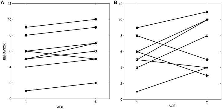
Figure 1. Differential consistency. (A) When differences among individuals in behavior are maintained over age or time, differential consistency (broad-sense repeatability) is high (r = 0.94). (B) When differences among individuals in behavior change over age or time, differential consistency is lower (r = 0.37).

Although the differential consistency of personality traits may be high when behavior is measured over short periods of time, it is often lower when measured over longer periods (Roberts and Delvecchio, 2000; Caspi et al., 2005; Stamps and Groothuis, 2010a; Boulton et al., 2014; Riemer et al., 2014). Also, when differential consistency is measured at different periods over the lifetime, it often varies as a function of age. In some species, the differential consistency of personality traits increases with age, i.e., personality is more stable later in life than it is early in life (squid, Sinn et al., 2008; humans, Roberts and Delvecchio, 2000; Caspi et al., 2005; dogs, Fratkin et al., 2013; fish, Edenbrow and Croft, 2011). These observations raise the question of why personality traits that are temporally stable over short periods might be less so over ontogeny.

In free-living animals, one obvious reason why the temporal stability of personality might change over ontogeny is that individuals had different experiences during the period in question. It is clear that personality traits can change within individuals as a result of past experience (Stamps and Groothuis, 2010a,b) For instance, Madagascar hissing cockroaches (Gromphadorhina portentosa) repeatedly exposed to predators over a 5 week period eventually became shyer, on average, than comparable individuals with no such experience (McDermott et al., 2014). Hence, in free-living animals, individual differences in behavior at a given age could easily occur as a result of differences among them in past experiences. However, this cannot be the whole story, because changes in the differential consistency of personality traits over time are observed even if all the subjects in a study are maintained from birth or hatching in captivity under highly standardized conditions (fish, Bell and Stamps, 2004; Edenbrow and Croft, 2011; squid, Sinn et al., 2008; insects, Gyuris et al., 2012; and primates, Sussman and Ha, 2011). Situations in which the differential consistency of personality changes over ontogeny, even when every subject has been exposed to the same (or at least very similar) experiential factors, imply that individuals differ with respect to the effects of the same experience on their behavioral development. In other words, changes in personality over time could be due to individual differences in developmental plasticity. More formally, in order to understand why personality might change over time, we need to understand individual differences in the developmental plasticity of personality traits. This is the topic explored in the current article.

We use a recent Bayesian model of behavioral development (Stamps and Krishnan, in press) to illustrate a number of basic principles relevant to individual differences in the developmental plasticity of personality traits. We begin with definitions of key concepts (i.e., behavioral developmental plasticity, potential, and realized plasticity) and then describe experimental protocols that empiricists have used to study individual differences in the developmental plasticity of behavior. A brief outline of the assumptions of the model is followed by a description of how it can be used to predict individual differences in developmental trajectories and the changes in the differential consistency of personality over ontogeny that result from those differences. We then show how the model can be used to illustrate the distinction between the potential and realized developmental plasticity of behavioral traits, and to show why relationships between initial scores for personality traits and the developmental plasticity of those traits would be expected to vary as a function of the cues to which individuals were exposed during ontogeny. Finally, we discuss the advantages and disadvantages of using different experimental protocols to estimate differences across individuals in the developmental plasticity of behavioral and other traits. We illustrate our main points by considering the development of boldness, a personality trait that has been studied in a wide range of animals, including humans (Fox et al., 2005; Reale et al., 2007; Conrad et al., 2011).

Definitions

When applied to behavior, the terms “plasticity” and “developmental plasticity” can be ambiguous because there are many different ways in which behavior can vary within individuals or genotypes as a result of variation in external stimuli (review in Stamps, under review). Here, we follow a longstanding tradition in ethology and psychology of discriminating between situations in which behavior varies as an immediate response to changes in external stimuli (contextual plasticity or activational plasticity) and situations in which behavior varies as a function of changes in external stimuli, experiences or environmental conditions that occurred in the past (developmental plasticity) (Stamps and Groothuis, 2010a; Snell-Rood, 2013). When applied to behavior, the term developmental plasticity encompasses a very wide range of phenomena, including learning, acclimation, and life-cycle staging (sensu Piersma and Drent, 2003), as well as situations in which experiences early in life affect the behavior expressed later in life. Since the current article is primarily concerned with gradual changes in personality that occur over ontogeny, it focuses on situations in which repeated or continuous exposure to specific types of experiential factors over extended periods of time affect the development and expression of personality traits.

When discussing the developmental plasticity of behavioral traits, it is also important to distinguish between potential and realized plasticity. Potential plasticity refers to the ability of an individual or a genotype to change its phenotype in response to changes in external stimuli, experiences, or environmental conditions, while realized plasticity refers to the change in phenotype that is actually observed when a given individual or genotype has been exposed to a specific set of external stimuli, experiences or environmental conditions (Stamps, under review). Potential plasticity is a construct that is central to theories on the evolution and ecological significance of individual differences in plasticity. This is because theoreticians often assume that individuals with high potential plasticity pay costs of maintaining the “machinery” that allows them to detect, monitor and respond to different stimuli, and that these maintenance costs of plasticity are paid even if the individual never expresses that plasticity (DeWitt et al., 1998; Auld et al., 2010). In contrast, realized plasticity is what empiricists actually measure in a given experiment. Concepts similar to potential and realized plasticity have been mentioned in passing by other authors. For instance, Ydenberg and Prins (2012) defined “flexibility” as the ability to adjust foraging behavior as circumstances change, but then noted that flexible individuals might not actually change their behavior if their original behavior performed well under the new set of conditions. Similarly, a recent theoretical model of the effects of phenotypic plasticity on population dynamics distinguished between the range of phenotypes that an individual is able to generate (plasticity-range), and the extent to which an individual's phenotype actually changes in a given situation (plasticity-used) (Gomez-Mestre and Jovani, 2013).

Understandably, empiricists often assume that their estimates of the realized plasticity of different individuals map directly onto the potential plasticity of those individuals. For instance, Thomson et al. (2012) found that initially shy rainbow trout (Oncorhynchus mykiss) did not significantly alter their level of boldness in response to a week's exposure to cues from a predator, and interpreted their results as indicating that shy fish were unable to respond to external cues. However, as we show below, the extent to which estimates of realized developmental plasticity reflect potential developmental plasticity can vary, depending on the experimental design that is used to measure differences among individuals or agents in developmental plasticity.

Experimental Designs for Studying the Developmental Plasticity of Personality Traits

Two experimental designs have traditionally been used to study the developmental plasticity of behavior: within-individual (or longitudinal) designs, and “common garden” designs. In within-individual designs, the behavior of the same agents is repeatedly measured at different ages. If subjects are repeatedly measured in the field, the resulting data simply describe how behavior of individual animals and the differential consistency of the individuals within the group changes as a function of age (e.g., Lucas and Donnellan, 2011; Petelle et al., 2013). However, if subjects are studied under carefully controlled conditions in the laboratory, within-individual designs can be used to describe how specific types of external stimuli, experiential factors, or environmental conditions affect the behavioral developmental trajectories of each of the subjects.

Within-individual designs are routinely used to describe individual differences in learning rates (Bell and Peeke, 2012; Thornton and Lukas, 2012), but they can also be used to study individual differences in other types of developmental plasticity, including the developmental plasticity of personality. For instance, by assessing the boldness of the same individuals before and after a period of exposure to cues from predators, researchers can use the difference between the two scores to estimate how each subject's boldness changed as a result of this experience (Bell and Sih, 2007; Thomson et al., 2012; Frost et al., 2013). Similarly, by repeatedly measuring the boldness of individuals reared in a “safe” environment (i.e., raised without any cues from predators, dangerous conspecifics, or other sources of danger), researchers can describe how the boldness of individuals or genotypes changes over the juvenile period as a function of this type of experience (Edenbrow and Croft, 2011; Sussman and Ha, 2011).

In the simplest type of within-individual design, subjects are consistently or repeatedly exposed to one set of cues or experiential factors over the entire study period. A slightly more complicated design involves first exposing subjects for an extended period to one set of cues or experiences, and then exposing them for a second extended period to a different set of cues or experiences. We will consider how both of these within-individual protocols can be used to study individual differences in the developmental plasticity of personality traits.

The second important way to investigate individual differences in developmental plasticity is to use a specific type of common garden experimental design, referred to here as a “replicate individual design.” In this version of a common garden experiment, replicate individuals are used as surrogates for individual animals. Replicate individuals are individuals with the same genotype (e.g., clones, isolines, or more approximately, siblings), raised under the same conditions prior to the beginning of an experiment (Stamps and Groothuis, 2010a). Replicate individuals not only share genes, but also important experiential factors (e.g., maternal or sibling effects) that typically vary more among than within genotypes. If such genotypes are derived from individuals randomly sampled from the same population, and have not been subsequently exposed to artificial selection, they can provide a powerful tool for studies of individual differences in various types of behavioral plasticities (Stamps, under review).

When replicate individuals are used to study behavioral development, they allow researchers to estimate how the behavior of each individual would have differed if that individual had been exposed to different experiences earlier in life. To this end, individuals with the same age and genotype are randomly assigned to different treatments. Then the individuals in each treatment are exposed to a different set of stimuli, experiential factors or environmental conditions for a specified period of time. Finally, the behavior of all of the subjects is measured using standard assays at the same age later in life.

Replicate individual designs have, of course, been widely used to study genotypic differences in the developmental plasticity of morphological and life history traits (e.g., Auld et al., 2010). However, they can also be used to describe differences among genotypes in the developmental plasticity of behavior. For instance, researchers have used replicate individual designs to document differences among isolines of Drosophila melanogaster in the effects of the larval rearing medium on adult responses to olfactory stimuli (Sambandan et al., 2008), differences among isolines of D. simulans in the effects of rearing temperature on female choosiness and mate preferences (Ingleby et al., 2013), and differences among paternal half-sibs of waxmoths (Achroia grisella) in the effects of density, temperature, and food levels during the larval period on adult male calling song (Zhou et al., 2008).

Model Description

We only briefly summarize the main assumptions of the model here, since details of the model are available elsewhere (Stamps and Krishnan, in press). We assume that at the time of birth or hatching, individuals already possess information about conditions in the external world, information provided to them by their distant ancestors (e.g., via genes, Leimar et al., 2006; Shea, 2007) and by their immediate ancestors (e.g., via inherited epigenetic factors and maternal effects, Uller, 2008; Shea et al., 2011; Keiser and Mondor, 2013; Burton and Metcalfe, 2014). We assume that at birth or hatching, different individuals in the same population begin life with different information from their ancestors, but that after birth or hatching, all individuals have the same personal experiences, which also provide them with information about conditions in the external world. The key assumption of our model is that, within each individual, information from its ancestors and information from a series of personal experiences is combined over ontogeny through Bayesian-like processes to affect behavior. The model focuses on personal experiences (cues) that provide information about the external world but do not directly affect the resources available for growth and development. For instance, it would apply to experiments in which animals were repeatedly exposed to stimuli from predators or conspecifics, but not to experiments in which the “experience” consisted of restricted food rations or infection by pathogens.

As is the case for any Bayesian model of behavior, our model includes four basic components: prior distributions, posterior distributions, likelihood functions and response functions. Informally, a prior distribution specifies an individual's beliefs about a biologically relevant variable (e.g., the state of danger) before it has a given experience (e.g., exposure to cues from a predator), and a posterior distribution specifies that individual's beliefs about that same variable after it has had that experience. The likelihood function for a particular type of experience specifies the probability that that experience would occur, given each possible state of the variable; the response function links belief to action, by specifying the relationship between an individual's current belief (based on its prior or its posterior distribution) and the behavior it expresses based on that belief. Importantly, the posterior distribution after one experience becomes the prior distribution for the next experience. This is why Bayesian approaches are useful for modeling development, where it is typical for a given individual to have a series of experiences over ontogeny, each of which may provide additional information about the state of the world (Frankenhuis and Panchanathan, 2011a,b; Fischer et al., 2014).

The current model assumes that at birth or hatching, individuals have different prior distributions, and that both the variable that individuals are attempting to estimate in the external environment (e.g., the state of danger) and the individuals' behavioral response to that estimate (e.g., their level of boldness) are continuously distributed. When combined, these two assumptions allow us to model personality traits, which may be expressed soon after birth or hatching, and which usually vary continuously across individuals within populations. These assumptions set our model apart from other recent Bayesian models of development, which assume that (1) all of the individuals in a population are born with the same prior distribution, (2) the variable in the external world that animals are attempting to estimate can take on one of only two different states, and (3) there are only two phenotypes, each of which is favored in one of the two states (e.g., Frankenhuis and Panchanathan, 2011a; Fischer et al., 2014). In addition, our assumption that prior and posterior distributions are continuously distributed allows the means and the variances of these distributions to vary independently of one another (see below, Appendix and Discussion); this is not an option in two-state models, since in binomial distributions, the variance is a fixed function of the mean.

In our model, we assume that the variable in the external environment (here, the state of danger) varies continuously from 0 to 1 (we divide the interval from 0 to 1 into 100 equally spaced states for ease of numerical computation), and use beta distributions to describe both prior distributions and likelihood functions. Beta distributions use two parameters (α and β) to generate a wide variety of monotonically increasing, monotonically decreasing, unimodal (hump-shaped), and uniform distributions. We do not, however, consider U-shaped prior distributions or likelihood functions (α < 1 and β < 1), in which extremely high and extremely low values of the variable are both more likely to occur than any intermediate values of the variable. This is because situations in which both extreme values of a variable are more likely to occur than any intermediate value are more easily and appropriately modeled using two-state rather than multiple-state Bayesian models.

We focus on likelihood functions with intermediate reliability, where the term reliability indicates the extent to which a given cue is associated with different states of the variable. With respect to the current model, a cue with the lowest reliability would be one that was equally likely to occur at any of the 100 states of danger, while a cue with the highest reliability would be one that was only likely to occur at only one of the 100 states of danger. Cues with moderately reliable likelihood functions are most relevant for studying the development of personality because cues with very low reliability have little effect on the behavior of any individual, while cues with very high reliability encourage every individual to rapidly develop the same phenotype (Frankenhuis and Panchanathan, 2011a; Fischer et al., 2014), even if those individuals began with different prior distributions (Stamps and Krishnan, in press).

For simplicity, in this article we focus on linear response functions (for discussion of other response functions, see Stamps and Krishnan, in press). That is, we assume that there is a linear relationship between the mean of the prior or posterior distribution at a given age and the mean level of behavior expressed by an individual at that age. Depending on the variable and the behavior, this relationship can be positive or negative. We assume that the level of boldness exhibited by an individual is negatively related to its current estimate of the state of danger (see also Appendix).

In order to investigate how individuals with a range of prior distributions would respond to experiences with different likelihood functions, we use Matlab to model the developmental trajectories of 15 hypothetical individuals, each of which has a different prior distribution for the state of danger. Each individual's prior distribution is described by its mean (0.1, 0.3, 0.5, 0.7, and 0.9) and its variance (0.001, 0.02, and the maximum variance possible for the mean value, given the constraints on the beta distributions noted above). The maximum possible variance for each prior distribution depends on its mean value. For instance, for prior distributions with a mean of 0.1 or 0.9, the maximum variance = 0.0426; whereas for prior distributions with a mean of 0.3 or 0.7, the maximum variance = 0.0864. For a prior distribution with a mean of 0.5, the maximum variance = 0.0833; this is the special case of a uniform distribution (α = 1, β = 1), in which each of the 100 possible states is equally likely to occur. Together, these 15 distributions span the range of prior distributions that are possible under the assumptions of our model.

We assume that each of the 15 individuals begins with a different prior distribution at birth or hatching (at age 0), and that the behavior expressed by each individual at age 0 is directly related to the mean of its prior distribution. Then all of the individuals are exposed to the same cues (same likelihood function) from age 0 to age 1. Each individual's posterior distribution at age 1 is computed by combining its prior distribution with the likelihood function using Bayes' equation, and its behavior at age 1 is assumed to be directly related to the mean of its posterior distribution at age 1. Each individual's posterior distribution at age 1 then becomes its prior distribution for the next experience (from age 1 to age 2). The procedure outlined above is then repeated to generate the posterior distributions and the expected behavior of each individual for each age from 2 to 4, as a function of their prior distributions at birth or hatching, and the likelihood functions for the cues to which they were exposed over the course of ontogeny.

Previous analyses have shown that when prior distributions are continuously distributed, the effects of a given cue (i.e., a given likelihood function) on the development of behavior depend on the mean and the variance of the prior distribution (Stamps and Krishnan, in press). If a prior distribution has low variance, behavior is not expected to change much, if at all, after any cue, regardless of the mean of the prior distribution or the shape of the likelihood function. In contrast, if a prior distribution has high variance, the extent to which a given cue affects behavior depends on the discrepancy between the mean of the prior distribution and the information about the state provided by the likelihood function. An intuitive explanation for these patterns is provided in the Appendix; see also Results.

Results

Within-Individual Designs for Describing the Developmental Plasticity of Personality Traits as a Function of Experience

Repeated exposure to cues with the same likelihood function

In this section, we assume that individuals with 15 different prior distributions for the state of danger are continuously or repeatedly exposed to the same cues (same likelihood function) from birth or hatching until the end of the juvenile period (see also Stamps and Krishnan, in press). The boldness of each individual is assessed soon after birth, and then again at a series of different ages. The developmental plasticity of boldness of each individual can then be estimated by the slope or shape of its developmental trajectory, either for a portion of ontogeny (e.g., from age 0 to age 1) or across the entire study period (e.g., from age 0 to age 4).

In the current study, we compare the results from three simulated experiments, in which a set of individuals with the same initial prior distributions are either repeatedly exposed to cues indicating that level of danger in the current environment is relatively low (Figure 2), to cues indicating that the level of danger is relatively high (Figure 3), or to cues indicating that the level of danger is intermediate (Figure 4).

FIGURE 2

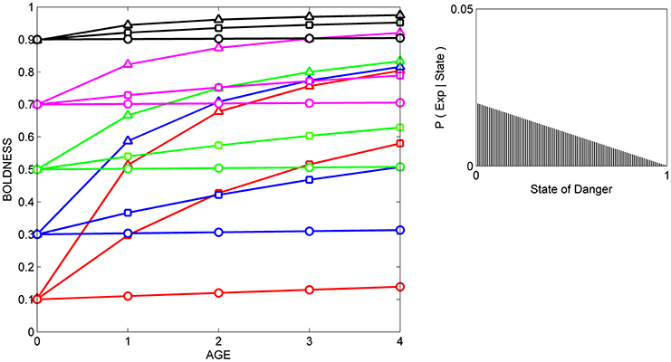
Figure 2. Developmental trajectories for boldness resulting from repeated exposure to cues indicative of safety. Fifteen hypothetical individuals with different prior distributions at birth are repeatedly exposed to the same cue, and their boldness is recorded at 5 ages across ontogeny. The mean of each prior distribution (and the resulting mean level of behavior at age 0) is indicated by color (red: 0.1, blue: 0.3, green: 0.5, magenta: 0.7, black: 0.9); the variance of each prior distribution is indicated by symbols (circles: variance = 0.001, squares, variance = 0.02; triangles, variance = maximal variance for each mean). The likelihood function (right box) indicates the probability of experience given the state (P (Exp|State) for each of the 100 possible states, ranging from 0 to 1. This likelihood function is moderately reliable and left-biased (i.e., the cue is more likely to occur when danger is low than when danger is moderate to high); it was generated by a beta distribution in which α = 2 and β = 1.

FIGURE 3

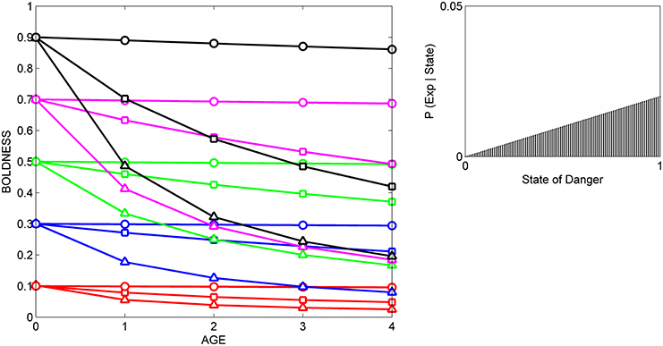
Figure 3. Developmental trajectories for boldness resulting from repeated exposure to a moderately reliable cue indicative of danger. Symbols for prior distributions as in Figure 2. The likelihood function (right box) was generated by a beta distribution with α = 1 and β = 2.

FIGURE 4

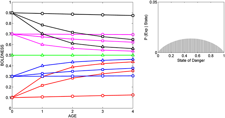
Figure 4. Developmental trajectories for boldness resulting from repeated exposure to a moderately reliable cue indicative of intermediate levels of danger. Symbols for prior distributions as in Figure 2. The likelihood function (right box) was generated by a beta distribution with α = 1.75 and β = 1.75.

In all three situations, scores for boldness tend to converge on the level of boldness that is encouraged by the likelihood function. That is, if cues indicate that the state of danger is low (Figure 2), most individuals gradually become bolder, if cues indicate that the state of danger is high, most individuals gradually become shyer (Figure 3), and if cues indicate that the state of danger is intermediate (Figure 4), most shy individuals gradually become bolder and most bold individuals gradually become shyer.

The variance and mean of each individual's prior distribution together determine how it will respond to a given cue. Individuals whose prior distributions had low variance (indicated by circles) maintain their initial level of boldness across ontogeny, regardless of the cues to which they are exposed. For instance, initially shy individuals whose prior distributions had low variance (red circles) remain shy, even if repeatedly exposed to cues indicating that the world is safe (Figure 2). In contrast, if individuals' prior distributions had high variance (indicated by triangles), their developmental trajectories depend on the relationship between the mean of their prior distribution and the likelihood function for the cue. An individual who was very shy at birth but whose prior distribution had a high variance (red triangles) becomes much bolder over ontogeny if raised with cues indicating that the world is relatively safe (Figure 2), remains shy over ontogeny if raised with cues indicating that the world is relatively dangerous (Figure 3), and becomes somewhat bolder if raised with cues indicating that the world is moderately safe (Figure 4). Of course, individuals can have prior distributions with variance anywhere between these two extremes: predicted developmental trajectories for individuals whose prior distributions had an intermediate variance of 0.02 are indicated by the lines with squares in Figures 2–4.

These predicted differences among individuals in their developmental trajectories for boldness follow directly from basic principles of Bayesian updating (see Appendix). Low variance for its prior distribution implies that, at birth, an individual is quite certain that the estimate of the state of danger provided by its ancestors is correct. Hence, the individual would continue to express the level of boldness encouraged by its prior distribution, even if repeatedly exposed to moderately reliable cues that imply that its initial level of boldness might not be appropriate in the current environment. In contrast, high variance for a prior distribution indicates that, at birth, an individual is very uncertain that the estimate of the state provided by its ancestors is correct. In that case, repeated exposure to moderately reliable cues can lead to a change in the level of boldness over ontogeny, but the extent to which behavior changes over time depends on the discrepancy between the estimate of the state of danger provided by the cue and the estimate of the state of danger provided by information from the individual's ancestors.

These patterns also provide a possible explanation for changes in the differential consistency of personality over ontogeny. The differential consistency of boldness for a given period (e.g., from age 0 to age 1) can be estimated by measuring the slope of each individual's developmental trajectory, and then quantifying the extent to which those slopes differ across the 15 individuals in the group. It can be easily seen that in Figures 2–4, the slopes of the developmental trajectories differ more across individuals earlier in life (from age 0 to age 1) than they do later in life (from age 3 to age 4). In other words, in the examples illustrated here, the model predicts that the differential consistency of personality will increase with age. Previous analyses indicate that differential consistency would increase with age for many other, though not all, likelihood functions and response functions (Stamps and Krishnan, in press; unpublished data).

In addition, the model predicts that relationships among individuals between personality traits and the developmental plasticity of those traits will vary, depending on the cues to which those individuals were exposed over ontogeny. More formally, across individuals, the relationship between initial scores for behavior (i.e., the intercepts of the development trajectories) and the absolute value (magnitude) of the slopes of the developmental trajectories depends on the likelihood function. For instance, in Figure 2, individuals with high initial scores are less plastic than individuals with low initial scores, as is indicated by the negative relationship across individuals between intercepts and the magnitude of the slopes across the entire study period (from age 0 to age 4). In contrast, in Figure 3, individuals with high initial scores are more plastic than those with low initial scores (a positive relationship, across individuals, between intercepts and the magnitude of the slopes), while in Figure 4, the relationship between intercept and the magnitude of the slopes is U-shaped: bold individuals become shyer, shy individuals become bolder, and intermediately bold individuals maintain their initial levels of behavior.

Finally, these results provide an easy way to grasp the distinction between potential plasticity and realized plasticity. The model indicates that the variance of an individual's prior distribution is directly related to its potential plasticity. Individuals whose prior distributions had low variance have low potential developmental plasticity, in the sense that they would not be expected to change their behavior much, if at all, in response to exposure to any cue over the course of development. In contrast, individuals whose prior distributions had high variance have high potential plasticity, because they are capable of major changes in behavior as a function of exposure to cues during development. Individuals whose prior distributions had intermediate variance have intermediate potential plasticity: they are able to change their behavior as a result of exposure to cues, but to a lesser extent for any given cue than individuals whose prior distributions had high variance.

However, it is also clear from comparison of Figures 2–4 that individuals with high potential plasticity do not necessarily always exhibit high realized plasticity. Instead, individuals whose prior distributions had high variance may express low realized plasticity, intermediate realized plasticity, or high realized plasticity, depending on the extent to which the estimate of the state provided by their prior distribution contradicts the estimate of the state provided by the cues to which they are exposed. For instance, a potentially plastic individual who initially estimated that the state of danger is intermediate (green triangles) would not be expected to change its level of boldness over ontogeny if exposed to cues that confirmed this initial estimate (Figure 4), but would be expected to either increase or decrease its level of boldness if exposed over ontogeny to cues that contradicted this initial estimate (Figures 2, 3).

Sequential exposure to cues with opposing likelihood functions

In this section we consider a slightly more complicated situation, in which individuals are first exposed to one cue (with one likelihood function) for an extended period over ontogeny and then are exposed to a different cue (with a different likelihood function) for a second extended period. We focus on situations in which the likelihood functions are biased in different directions, because if different cues or experiences have similar likelihood functions, they are predicted to have comparable effects on developmental trajectories.

In the first example (Figure 5A), individuals born with a range of prior distributions are first exposed from age 0 to age 2 to a cue with a moderately reliable left-biased likelihood function (i.e., a cue that indicates that the state of danger is relatively low) and are then exposed from age 2 to age 4 to a different moderately reliable cue with a right-biased likelihood function (i.e., a cue indicating that the state of danger is relatively high). As one would expect, across all of the subjects, average boldness first gradually increases when individuals are exposed to cues indicative of safety, and then average boldness gradually declines when individuals are exposed to cues indicative of danger. Also, as one would expect from the discussion in the previous section, individuals with low potential plasticity (prior distributions with low variance) do not change their behavior in response to either type of experience.

FIGURE 5

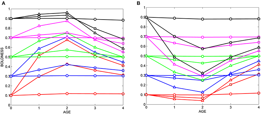
Figure 5. Sequential exposure to cues with different likelihood functions. (A) Fifteen hypothetical individuals are first exposed from age 0 to age 2 to cues indicating that the world is relatively safe (see box in Figure 2), then are exposed from age 2 to age 4 to cues indicating that the world is relatively dangerous (see box in Figure 3). (B) Individuals with the same prior distributions are first exposed from age 0 to age 2 to cues indicating that the world is relatively dangerous (box, Figure 3), then to cues indicating that the world is relatively safe (box, Figure 2). Symbols for prior distributions as in Figure 2.

However, some of the other patterns illustrated in Figure 5A are less intuitive. For instance, even though both likelihood functions are equally informative (same shape, albeit biased in opposite directions, see boxes in Figures 2, 3), following exposure to both cues, individuals with moderate to high potential plasticity do not end up with the same level of boldness that they had at birth or hatching (at age 0). Instead, scores for boldness tend to converge on the intermediate values that are appropriate for both likelihood functions. And, despite the change in cues and likelihood functions midway through ontogeny, differential consistency tends to increase as a function of age: the variance across individuals in the slopes of their developmental trajectories is higher from age 0 to age 1 than it is from age 3 to age 4. Thus, several of the patterns expected when individuals are exposed to a single cue through ontogeny are also observed if cues reverse midway through ontogeny.

With respect to providing reasonable estimates of potential developmental plasticity, the sequential within-individual design does a better job than a simpler experimental protocol in which individuals are exposed to just one cue over ontogeny. This is because individuals with high potential plasticity whose behavior is unaffected by initial exposure to a cue with a likelihood function biased in one direction would be expected to change their behavior when exposed to a different cue with a likelihood function biased in the opposite direction. For instance, the potentially plastic “bold” individual indicated by the black triangles in Figure 5A maintains its initial level of high boldness (low realized plasticity) as long as it is exposed to cues indicative of safety, but subsequently reduces its level of boldness (high realized plasticity) when it is repeatedly exposed to cues indicative of danger.

However, one problem with using sequential within-individual designs to estimate potential plasticity is that the order in which individuals are exposed to each of a series of cues affects their responses to those cues. This can be seen easily by using the range of scores each individual expresses over ontogeny to estimate its realized plasticity. For instance, in Figure 5A, the individual indicated by the red triangles has scores which range from a minimum of 0.1 to a maximum of 0.68 over the period from age 0 to age 4, so it has higher realized plasticity than the individual indicated by the blue squares, whose scores range from 0.3 to 0.4 over the same period. By extension, we can use this method to compare the realized plasticity of individuals with the same prior distribution who were sequentially exposed to the same two cues, but in a different order (Figure 5A vs. Figure 5B). This process shows that the realized plasticity of equivalent individuals depends on the order in which they were exposed to the same cues. For instance, the initially shy individual indicated by the red triangles is more plastic in Figure 5A (range of boldness scores: 0.1–0.68) than is the equivalent individual in Figure 5B (range of scores: 0.05–0.42). As a result of these differences, the rank-order of realized plasticity for the individuals in the two groups varies as a function of cue order. For example, the individual with the highest realized plasticity in Figure 5A is the initially shy individual indicated by the red triangles, but the individual with the highest realized plasticity in Figure 5B is the initially bold individual indicated by the black triangles.

The order in which individuals are sequentially exposed to cues over ontogeny affects their realized plasticity because, by its very nature, Bayesian updating incorporates information from the past when estimating the current state of the world (see Appendix, and references on Bayesian updating in Stamps and Krishnan, in press). The notion that order matters when subjects are sequentially exposed to different cues or experiences is quite familiar to empiricists studying another type of developmental plasticity, learning. For instance, in reversal learning experiments, acquisition rates for the first response in the sequence are often different from the acquisition rates for the second response, following the change in the task contingency (e.g., Colwill et al., 2005; Moy et al., 2007; Shettleworth, 2010; Lloyd and Leslie, 2013).

The fact that order matters when individuals are exposed to different cues over ontogeny implies that although sequential within-individual designs provide better estimates of potential developmental plasticity than within-individual designs that only utilize one cue, there may still be substantial discrepancies between the estimates of realized developmental plasticity provided by this method and the potential plasticity of the subjects.

Replicate Individual Designs

Common garden experiments using replicate individuals as subjects (i.e., replicate individual designs) measure developmental plasticity differently than is the case for within-individual (longitudinal) experimental designs. Instead of describing how the behavior of each individual changes over time as a function of exposure to a given experience (or sequence of experiences), the scores of matched individuals who have been exposed to different experiences over the same period of time are compared to one another.

A little thought reveals that replicate individual designs are equivalent to simultaneously conducting two or more of the experiments outlined above, except that in this case, the subjects are genotypes (replicate individuals) rather than individual animals. For instance, imagine that one set of representatives of 15 genotypes were raised in the presence of cues indicative of safety (Figure 2), and a second matched set of the same genotypes were raised in the presence of cues indicative of danger (Figure 3). Then, at age 4, boldness is assessed for each of the subjects in each treatment. The resulting data could then be used to estimate each genotype's developmental response to each set of cues, as indicated in Figure 6. Note that instead of plotting the behavior of each agent as a function of age or time, we now plot the mean behavior of each genotype at age 4, as a function of the cues to which they were exposed earlier in life: treatment 1 (reared with cues indicative of safety), vs. treatment 2 (reared with cues indicative of danger).

FIGURE 6

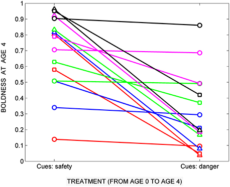
Figure 6. A hypothetical common garden experiment showing how exposure to cues in two different rearing treatments might affect the boldness of 15 genotypes (replicate individuals). Genotypes with the prior distributions specified by the symbols in Figure 2 are either raised with cues indicative of safety (see Figure 2) or with cues indicative of danger (see Figure 3). The mean boldness scores at age 4 are compared for the two treatment groups. Realized developmental plasticity is lowest for genotypes whose prior distributions had low variance (circles), intermediate for genotypes whose prior distributions had intermediate variance (squares) and highest for genotypes whose prior distributions had high variance (triangles).

In the simplest replicate individual design, in which matched genotypes are raised in two different treatments and their trait values are compared at the end of the study, the plasticity of each genotype is indicated by the difference between its scores in the two treatments (see Auld et al., 2010). It can be seen that this procedure provides reasonable estimates of the potential plasticity of the 15 genotypes in this study (Figure 6). Genotypes whose prior distributions had low variance (circles) have low plasticity: there is little or no difference in their scores at age 4 after being reared in the two treatments. Genotypes whose prior distributions had intermediate variance (squares) have moderately lower boldness scores after treatment 2 than after treatment 1, while genotypes whose prior distributions had high variance (triangles) have much lower boldness scores after treatment 2 than after treatment 1.

Generally speaking, replicate individual designs have several advantages over within-individual designs with respect to estimating the potential developmental plasticity of different agents. Because individuals with the same genotype can be exposed over ontogeny to two (or more) different treatments, individuals with high potential plasticity are expected to change their behavior in response to at least one of them. This is in contrast to the situation when subjects are exposed to just one cue throughout the experiment, since in the latter situation individuals with high potential plasticity may have low realized plasticity if raised with cues that indicate that their initial phenotype was appropriate for the current environment. And, because each set of replicate individuals is reared under a single set of conditions, the order effects that can complicate sequential, within-individual designs are not a concern in replicate individual designs.

On the other hand, information about temporal change in behavior is lost in traditional replicate individual designs. This is because in such designs, the behavior of the different replicate individuals is typically not measured soon after birth or hatching, so there is no way to estimate the extent to which the behavior of each agent changed over ontogeny. Of course, there are also a number of practical issues with replicate individual designs, e.g., replicate individuals are more readily available in some species than others, and because behavior can vary among individuals with the same genotype, large numbers of individuals per genotype may be required to obtain reliable estimates of the behavior of each genotype. These issues are discussed in more detail in Stamps, under review.

Discussion and Conclusions

The current article shows that a simple Bayesian model can be very useful for illustrating concepts relevant to the development of personality. It explains why one would expect to see individual differences in the developmental trajectories of personality traits and changes in the differential consistency of personality over ontogeny, even if every subject was raised under the same set of conditions. It shows why we would expect relationships between initial personality scores and the developmental plasticity of personality to vary among empirical studies, as a function of the cues to which those subjects were exposed during those studies. More broadly, it highlights the distinction between realized and potential plasticity, and indicates why certain experimental protocols for studying the developmental plasticity of behavioral traits might provide better estimates than others of the potential plasticity of different individuals or genotypes. In addition, the model may have practical value, in terms of predicting the developmental trajectories of personality traits of individuals or genotypes. This topic is explored in greater detail in Stamps and Krishnan (in press), which discusses ways to estimate the mean and variance of an agent's prior distribution, based on the mean level of behavior, and the short-term spontaneous variability of behavior (intra-individual variability (IIV), or intra-genotypic variability) that it expresses soon after birth or hatching.

Another insight from the model is that different experimental designs provide different information about individual differences in the developmental plasticity of behavioral traits. Within-individual (longitudinal) designs provide the data required to describe individual developmental trajectories and changes in the differential consistency of behavioral traits over ontogeny, but they provide less reliable estimates of the potential plasticity of different individuals or genotypes than do replicate individual designs. Conversely, although traditional replicate individual designs can provide reasonable estimates of the potential plasticity of different replicate individuals (genotypes), they don't provide information about how personality changes as a function of age. In species and situations in which replicate experimental designs are impractical, our analyses suggest that sequential within-individual designs (in which cues switch midway through ontogeny) are more likely to provide reasonable estimates of potential plasticity than are within-individual designs in which the subjects are reared with the same cues throughout ontogeny. In species and situations in which replicate individual designs are feasible, we suggest using hybrid experimental designs, i.e., common garden experiments in which the behavior of the subjects is measured before they are placed in the different treatment groups, and then measured again at regular intervals over the study (e.g., Edenbrow and Croft, 2013). With sufficient statistical power, this type of hybrid design can not only provide estimates of the potential plasticity of different replicate individuals, but also provide estimates of the shapes or the slopes of their behavioral developmental trajectories.

Although experimental studies of individual differences in the developmental trajectories of personality traits are still quite limited, there is some support for the model's general prediction that relationships between initial scores for personality traits and the subsequent plasticity of those traits might vary as a function of the cues to which individuals were exposed over ontogeny. For instance, when pigtailed macaques, Macaca nemestrina and clones (genotypes) of Mangrove killifish, Kryptolebias marmoratus were raised in the absence of cues indicative of danger, the average boldness of juveniles increased with age, but across individuals or genotypes, shy individuals became bolder and bold individuals remained relatively bold (Edenbrow and Croft, 2011; Sussman and Ha, 2011). Thus, the intercepts and the magnitude of the slopes of developmental trajectories for boldness were negatively related to one another, as predicted by the model (see Figure 2, also Stamps and Krishnan, in press). In contrast, when juvenile rainbow trout, Oncorhynchus mykiss, were repeatedly exposed to predators over a 2 week period, there was no change in their average boldness, but bold individuals became shyer, and shy individuals become bolder (Frost et al., 2013). This is the pattern predicted by our model if individuals with different initial levels of boldness were repeatedly exposed to cues indicative of an intermediate level of danger (e.g., see Figure 4). To our knowledge, to date no one has described the developmental trajectories for boldness for individuals or genotypes who initially expressed different levels of boldness, and who were then repeatedly or continuously exposed to cues indicative of high levels of danger. In this situation, our model predicts a decline in average boldness over ontogeny, and a positive relationship, across agents, between the intercepts and the magnitude of the slopes of developmental trajectories for boldness (e.g., see Figure 3).

Although boldness was used to illustrate the main points of this study, the same approach could be used to model the development of other personality traits (e.g., activity, exploratory behavior, aggressiveness). Similarly, although we have focused on cues that might affect individuals' estimates of the state of danger, cues associated with other variables in the external world (e.g., local population density, food availability, etc.) might also affect the development of personality traits. In principle, the general approach outlined in the current study could apply to any continuously variable labile behavioral or physiological trait. In practice, the major challenge for empiricists will be to begin their experiments already armed with reasonable assumptions about the likelihood functions for specific cues, and about the response functions that link prior distributions or posterior distributions with behavior.

In the current article we were able to build upon an extensive literature that indicates that cues from predators (or the lack thereof) convey information about the state of danger, and that levels of boldness should decline as estimates of the state of danger increase. However, it is not always obvious how behavior should change over ontogeny in response to continuous or repeated exposure to a given cue. For instance, there is empirical evidence that juvenile crickets use repeated exposure to acoustic signals from adult males to estimate the type of social environment they will later encounter as adults (see Bailey and Zuk, 2008; Kasumovic et al., 2011; DiRienzo et al., 2012). However, it is currently unclear how exposure to those cues should affect the development of aggressive behavior. Some authors have suggested that exposure to cues indicative of high densities of local competitors should favor the development of elevated levels of aggressiveness in male crickets (e.g., see DiRienzo et al., 2012). But cues indicating that the local neighborhood already contains many older, vigorously calling, territory owners might just as easily favor the development of reduced aggressiveness and enhanced subordinate behavior in callow, young males. This alternate hypothesis is suggested by empirical studies indicating that newly mature male crickets have difficulty competing aggressively with older, established territorial residents (e.g., Dixon and Cade, 1986; Buena and Walker, 2008; Rillich et al., 2011). In fact, preliminary results support the second hypothesis: male Gryllus integer reared with conspecific calls exhibited lower levels of aggressiveness as adults in standardized staged encounters than did males reared without them (DiRienzo et al., 2012). Hence, until more is known about the levels of aggressiveness favored when young male crickets emerge in localities with different densities of older, established territory owners, it would be premature to construct theoretical models based on assumptions about the effects of conspecific calls on the development of aggressiveness in this taxon.

Many of the assumptions which underlie the current study are not new, and can be found scattered among different literatures. These include (1) there is standing genetic variation within populations, not only in behavioral trait values but also in the potential plasticity of those traits (Wolf et al., 2008, 2011; Rodriguez, 2013), (2) information provided by parents about the environment can affect the development of personality traits (Reddon, 2012; Schuett et al., 2013), (3) information from ancestors and from personal experiences combines across ontogeny to affect the development of phenotypic traits (Leimar et al., 2006; Frankenhuis and Panchanathan, 2011a; Fischer et al., 2014), and (4) Bayesian-like mechanisms provide the optimal way to combine information from different sources (McLinn and Stephens, 2006; McNamara et al., 2006; Lange and Dukas, 2009). Our main contribution has been to combine these assumptions to generate predictions about individual differences in the developmental trajectories of continuously distributed phenotypic traits. One of the major insights to be gleaned from this approach is that variation among individuals and genotypes in the reliability of information provided by their ancestors may play as important a role as the reliability of information from personal experiences in determining how a given individual or genotype will respond to exposure to a given type of experience over the course of development. That is, our model suggests that an individual who assumes that the information from its ancestors is highly reliable (i.e., a prior distribution with low variance) would have lower potential plasticity than an individual who assumes that the information from its ancestors is less reliable (i.e., a prior distribution with high variance). Thus, our approach complements earlier theoretical studies which indicate that developmental plasticity can be limited by the reliability of the cues to which individuals are exposed over ontogeny (DeWitt et al., 1998; Tufto, 2000; Frankenhuis and Panchanathan, 2011a; Fischer et al., 2014). It expands upon those findings to show that even if every subject is exposed to the same (moderately reliable) cues over ontogeny, individual differences in developmental trajectories would still be expected if neonates start out with different information from their ancestors, a situation which is likely to be common in the natural world (Stamps and Krishnan, in press).

More generally, we suggest that a Bayesian perspective can be helpful for understanding a number of difficult concepts in development. It shows how genes, maternal effects, and personal experiences might iteratively interact with one another across ontogeny to affect the expression of behavior and other phenotypic traits (see also Oyama, 2000; Bateson and Gluckman, 2011). It emphasizes that information about the same state of the world can come from many different sources, at many different times across an individual's lifetime, and that information from genes does not have precedence over information from other sources (see Lickliter, 2008). It demonstrates that information from ancestors can continue to affect an individual's developmental trajectory, even after that individual has had a series of informative personal experiences, and suggests why some individuals might be more sensitive than others to the effects of the same experiential factors on their developmental trajectories. Hence, a Bayesian approach to development may have value that extends well beyond the specific questions addressed in the current study.

Conflict of Interest Statement

The Guest Associate Editor Ann Valerie Hedrick declares that, despite being affiliated with the same institution as author Judy Stamps, the review process was handled objectively and no conflict of interest exists. The authors declare that the research was conducted in the absence of any commercial or financial relationships that could be construed as a potential conflict of interest.

References

Auld, J. R., Agrawal, A. A., and Relyea, R. A. (2010). Re-evaluating the costs and limits of adaptive phenotypic plasticity. Proc. R. Soc. B 277, 503–511. doi: 10.1098/rspb.2009.1355

Pubmed Abstract | Pubmed Full Text | CrossRef Full Text | Google Scholar

Bailey, N. W., and Zuk, M. (2008). Acoustic experience shapes female mate choice in field crickets. Proc. R. Soc. B 275, 2645–2650. doi: 10.1098/rspb.2008.0859

Pubmed Abstract | Pubmed Full Text | CrossRef Full Text | Google Scholar

Bateson, P., and Gluckman, P. (2011). Plasticity, Robustness, Development and Evolution. New York, NY: Cambridge University Press. doi: 10.1017/CBO9780511842382

CrossRef Full Text | Google Scholar

Bell, A. M., and Peeke, H. V. S. (2012). Individual variation in habituation: behaviour over time toward different stimuli in threespine sticklebacks (Gasterosteus aculeatus). Behaviour 149, 1339–1365. doi: 10.1163/1568539X-00003019

CrossRef Full Text

Bell, A. M., and Sih, A. (2007). Exposure to predation generates personality in threespined sticklebacks (Gasterosteus aculeatus). Ecol. Lett. 10, 828–834. doi: 10.1111/j.1461-0248.2007.01081.x

Pubmed Abstract | Pubmed Full Text | CrossRef Full Text | Google Scholar

Bell, A. M., and Stamps, J. A. (2004). Development of behavioural differences between individuals and populations of sticklebacks, Gasterosteus aculeatus. Anim. Behav. 68, 1339–1348. doi: 10.1016/j.anbehav.2004.05.007

CrossRef Full Text | Google Scholar

Boulton, K., Grimmer, A. J., Rosenthal, G. G., Walling, C. A., and Wilson, A. J. (2014). How stable are personalities? A multivariate view of behavioural variation over long and short timescales in the sheepshead swordtail, Xiphophorus birchmanni. Behav. Ecol. Sociobiol. 68, 791–803. doi: 10.1007/s00265-014-1692-0

CrossRef Full Text | Google Scholar

Buena, L. J., and Walker, S. E. (2008). Information asymmetry and aggressive behaviour in male house crickets, Acheta domesticus. Anim. Behav. 75, 199–204. doi: 10.1016/j.anbehav.2007.04.027

CrossRef Full Text | Google Scholar

Burton, T., and Metcalfe, N. B. (2014). Can environmental conditions experienced in early life influence future generations? Proc. R. Soc. B 281:20140311. doi: 10.1098/rspb.2014.0311

Pubmed Abstract | Pubmed Full Text | CrossRef Full Text | Google Scholar

Caspi, A., Roberts, B. W., and Shiner, R. L. (2005). Personality development: stability and change. Annu. Rev. Psychol. 56, 453–484. doi: 10.1146/annurev.psych.55.090902.141913

Pubmed Abstract | Pubmed Full Text | CrossRef Full Text | Google Scholar

Colwill, R. M., Raymond, M. P., Ferreira, L., and Escudero, H. (2005). Visual discrimination learning in zebrafish (Danio rerio). Behav. Processes 70, 19–31. doi: 10.1016/j.beproc.2005.03.001

Pubmed Abstract | Pubmed Full Text | CrossRef Full Text | Google Scholar

Conrad, J. L., Weinersmith, K. L., Brodin, T., Saltz, J. B., and Sih, A. (2011). Behavioural syndromes in fishes: a review with implications for ecology and fisheries management. J. Fish Biol. 78, 395–435. doi: 10.1111/j.1095-8649.2010.02874.x

Pubmed Abstract | Pubmed Full Text | CrossRef Full Text | Google Scholar

Courville, A. C., Daw, N. D., and Touretzky, D. S. (2006). Bayesian theories of conditioning in a changing world. Trends Cogn. Sci. 10, 294–300. doi: 10.1016/j.tics.2006.05.004

Pubmed Abstract | Pubmed Full Text | CrossRef Full Text | Google Scholar

DeWitt, T. J., Sih, A., and Wilson, D. S. (1998). Costs and limits of phenotypic plasticity. Trends Ecol. Evol. 13, 77–81. doi: 10.1016/S0169-5347(97)01274-3

Pubmed Abstract | Pubmed Full Text | CrossRef Full Text | Google Scholar

DiRienzo, N., Pruitt, J. N., and Hedrick, A. V. (2012). Juvenile exposure to acoustic sexual signals from conspecifics alters growth trajectory and an adult personality trait. Anim. Behav. 84, 861–868. doi: 10.1016/j.anbehav.2012.07.007

CrossRef Full Text | Google Scholar

Dixon, K. A., and Cade, W. H. (1986). Some factors influencing male male aggression in the field cricket Gryllus integer (time of day, age, weight and sexual maturity). Anim. Behav. 34, 340–346. doi: 10.1016/S0003-3472(86)80102-6

CrossRef Full Text | Google Scholar

Edenbrow, M., and Croft, D. P. (2011). Behavioural types and life history strategies during ontogeny in the mangrove killifish, Kryptolebias marmoratus. Anim. Behav. 82, 731–741. doi: 10.1016/j.anbehav.2011.07.003

CrossRef Full Text | Google Scholar

Edenbrow, M., and Croft, D. P. (2013). Environmental and genetic effects shape the development of personality traits in the mangrove killifish Kryptolebias marmoratus. Oikos 122, 667–681. doi: 10.1111/j.1600-0706.2012.20556.x

CrossRef Full Text | Google Scholar

Fischer, B., Van Doorn, G. S., Dieckmann, U., and Taborsky, B. (2014). The evolution of age-dependent plasticity. Am. Nat. 183, 108–125. doi: 10.1086/674008

Pubmed Abstract | Pubmed Full Text | CrossRef Full Text | Google Scholar

Fox, N. A., Henderson, H. A., Marshall, P. J., Nichols, K. E., and Ghera, M. M. (2005). Behavioral inhibition: linking biology and behavior within a developmental framework. Annu. Rev. Psychol. 56, 235–262. doi: 10.1146/annurev.psych.55.090902.141532

Pubmed Abstract | Pubmed Full Text | CrossRef Full Text | Google Scholar

Frankenhuis, W. E., and Panchanathan, K. (2011a). Balancing sampling and specialization: an adaptationist model of incremental development. Proc. R. Soc. B 278, 3558–3565. doi: 10.1098/rspb.2011.0055

Pubmed Abstract | Pubmed Full Text | CrossRef Full Text | Google Scholar

Frankenhuis, W. E., and Panchanathan, K. (2011b). Individual differences in developmental plasticity may result from stochastic sampling. Perspect. Psychol. Sci. 6, 336–347. doi: 10.1177/1745691611412602

Pubmed Abstract | Pubmed Full Text | CrossRef Full Text | Google Scholar

Fratkin, J. L., Sinn, D. L., Patall, E. A., and Gosling, S. D. (2013). Personality consistency in dogs: a meta-analysis. PLoS ONE 8:e54907. doi: 10.1371/journal.pone.0054907

Pubmed Abstract | Pubmed Full Text | CrossRef Full Text | Google Scholar

Frost, A. J., Thomson, J. S., Smith, C., Burton, H. C., Davis, B., Watts, P. C., et al. (2013). Environmental change alters personality in the rainbow trout, Oncorhynchus mykiss. Anim. Behav. 85, 1199–1207. doi: 10.1016/j.anbehav.2013.03.006

CrossRef Full Text | Google Scholar

Gomez-Mestre, I., and Jovani, R. (2013). A heuristic model on the role of plasticity in adaptive evolution: plasticity increases adaptation, population viability and genetic variation. Proc. R. Soc. B 280:20131869. doi: 10.1098/rspb.2013.1869

Pubmed Abstract | Pubmed Full Text | CrossRef Full Text | Google Scholar

Gyuris, E., Fero, O., and Barta, Z. (2012). Personality traits across ontogeny in firebugs, Pyrrhocoris apterus. Anim. Behav. 84, 103–109. doi: 10.1016/j.anbehav.2012.04.014

Pubmed Abstract | Pubmed Full Text | CrossRef Full Text | Google Scholar

Hayes, J. P., and Jenkins, S. H. (1997). Individual variation in mammals. J. Mammal. 78, 274–293. doi: 10.2307/1382882

CrossRef Full Text | Google Scholar

Ingleby, F. C., Hunt, J., and Hosken, D. J. (2013). Genotype-by-environment interactions for female mate choice of male cuticular hydrocarbons in Drosophila simulans. PLoS ONE 8:e67623. doi: 10.1371/journal.pone.0067623

Pubmed Abstract | Pubmed Full Text | CrossRef Full Text | Google Scholar

Kasumovic, M. M., Hall, M. D., Try, H., and Brooks, R. C. (2011). The importance of listening: juvenile allocation shifts in response to acoustic cues of the social environment. J. Evol. Biol. 24, 1325–1334. doi: 10.1111/j.1420-9101.2011.02267.x

Pubmed Abstract | Pubmed Full Text | CrossRef Full Text | Google Scholar

Keiser, C. N., and Mondor, E. B. (2013). Transgenerational behavioral plasticity in a parthenogenetic insect in response to increased predation risk. J. Insect Behav. 26, 603–613. doi: 10.1007/s10905-013-9376-6

CrossRef Full Text | Google Scholar

Lange, A., and Dukas, R. (2009). Bayesian approximations and extensions: optimal decisions for small brains and possibly big ones too. J. Theor. Biol. 259, 503–516. doi: 10.1016/j.jtbi.2009.03.020

Pubmed Abstract | Pubmed Full Text | CrossRef Full Text | Google Scholar

Leimar, O., Hammerstein, P., and Van Dooren, T. J. M. (2006). A new perspective on developmental plasticity and the principles of adaptive morph determination. Am. Nat. 167, 367–376. doi: 10.1086/499566

Pubmed Abstract | Pubmed Full Text | CrossRef Full Text | Google Scholar

Lickliter, R. (2008). The growth of developmental thought: implications for a new evolutionary psychology. New Ideas Psychol. 26, 353–369. doi: 10.1016/j.newideapsych.2007.07.015

Pubmed Abstract | Pubmed Full Text | CrossRef Full Text | Google Scholar

Lloyd, K., and Leslie, D. S. (2013). Context-dependent decision-making: a simple Bayesian model. J. R. Soc. Interface 10:20130069. doi: 10.1098/rsif.2013.0069

Pubmed Abstract | Pubmed Full Text | CrossRef Full Text | Google Scholar

Lucas, R. E., and Donnellan, M. B. (2011). Personality development across the life span: longitudinal analyses with a national sample from Germany. J. Pers. Soc. Psychol. 101, 847–861. doi: 10.1037/a0024298

Pubmed Abstract | Pubmed Full Text | CrossRef Full Text | Google Scholar

McDermott, D. R., Chips, M. J., McGuirk, M., Armagost, F., Dirienzo, N., and Pruitt, J. N. (2014). Boldness is influenced by sublethal interactions with predators and is associated with successful harem infiltration in Madagascar hissing cockroaches. Behav. Ecol. Sociobiol. 68, 425–435. doi: 10.1007/s00265-013-1657-8

CrossRef Full Text | Google Scholar

McGraw, K. O., and Wong, S. P. (1996). Forming inferences about some intraclass correlation coefficients. Psychol. Methods 1, 30–46. doi: 10.1037/1082-989X.1.4.390

CrossRef Full Text | Google Scholar

McLinn, C. M., and Stephens, D. W. (2006). What makes information valuable: signal reliability and environmental uncertainty. Anim. Behav. 71, 1119–1129. doi: 10.1016/j.anbehav.2005.09.006

CrossRef Full Text | Google Scholar

McNamara, J. M., Green, R. F., and Olsson, O. (2006). Bayes' theorem and its applications in animal behaviour. Oikos 112, 243–251. doi: 10.1111/j.0030-1299.2006.14228.x

CrossRef Full Text | Google Scholar

Moy, S. S., Nadler, J. J., Young, N. B., Perez, A., Holloway, L. P., Barbaro, R. P., et al. (2007). Mouse behavioral tasks relevant to autism: phenotypes of 10 inbred strains. Behav. Brain Res. 176, 4–20. doi: 10.1016/j.bbr.2006.07.030

Pubmed Abstract | Pubmed Full Text | CrossRef Full Text | Google Scholar

Nakagawa, S., and Schielzeth, H. (2010). Repeatability for Gaussian and non-Gaussian data: a practical guide for biologists. Biol. Rev. Camb. Philos. Soc. 85, 935–956. doi: 10.1111/j.1469-185X.2010.00141.x

Pubmed Abstract | Pubmed Full Text | CrossRef Full Text | Google Scholar

Oyama, S. (2000). The Ontogeny of Information: Developmental Systems and Evolution. Durham, NC: Duke University Press. doi: 10.1215/9780822380665

CrossRef Full Text | Google Scholar

Petelle, M. B., McCoy, D. E., Alejandro, V., Martin, J. G. A., and Blumstein, D. T. (2013). Development of boldness and docility in yellow-bellied marmots. Anim. Behav. 86, 1147–1154. doi: 10.1016/j.anbehav.2013.09.016

CrossRef Full Text | Google Scholar

Piersma, T., and Drent, J. (2003). Phenotypic flexibility and the evolution of organismal design. Trends Ecol. Evol. 18, 228–233. doi: 10.1016/S0169-5347(03)00036-3

Pubmed Abstract | Pubmed Full Text | CrossRef Full Text | Google Scholar

Reale, D., Reader, S. M., Sol, D., McDougall, P. T., and Dingemanse, N. J. (2007). Integrating animal temperament within ecology and evolution. Biol. Rev. Camb. Philos. Soc. 82, 291–318. doi: 10.1111/j.1469-185X.2007.00010.x

Pubmed Abstract | Pubmed Full Text | CrossRef Full Text | Google Scholar

Reddon, A. R. (2012). Parental effects on animal personality. Behav. Ecol. 23, 242–245. doi: 10.1093/beheco/arr210

CrossRef Full Text | Google Scholar

Riemer, S., Muller, C., Viranyi, Z., Huber, L., and Range, F. (2014). The predictive value of early behavioural assessments in pet dogs - a longitudinal study from neonates to adults. PLoS ONE 9:e101237. doi: 10.1371/journal.pone.0101237

Pubmed Abstract | Pubmed Full Text | CrossRef Full Text | Google Scholar

Rillich, J., Schildberger, K., and Stevenson, P. A. (2011). Octopamine and occupancy: an aminergic mechanism for intruder-resident aggression in crickets. Proc. R. Soc. B 278, 1873–1880. doi: 10.1098/rspb.2010.2099

Pubmed Abstract | Pubmed Full Text | CrossRef Full Text | Google Scholar

Roberts, B. W., and Delvecchio, W. F. (2000). The rank-order consistency of personality traits from childhood to old age: a quantitative review of longitudinal studies. Psychol. Bull. 126, 3–25. doi: 10.1037/0033-2909.126.1.3

Pubmed Abstract | Pubmed Full Text | CrossRef Full Text | Google Scholar

Rodriguez, R. L. (2013). Causes of variation in genotype x environment interaction. Evol. Ecol. Res. 15, 733–746.

Google Scholar

Sambandan, D., Carbone, M. A., Anholt, R. R. H., and Mackay, T. E. C. (2008). Phenotypic plasticity and genotype by environment interaction for olfactory behavior in Drosophila melanogaster. Genetics 179, 1079–1088. doi: 10.1534/genetics.108.086769

Pubmed Abstract | Pubmed Full Text | CrossRef Full Text | Google Scholar

Schuett, W., Dall, S. R. X., Wilson, A. J., and Royle, N. J. (2013). Environmental transmission of a personality trait: foster parent exploration behaviour predicts offspring exploration behaviour in zebra finches. Biol. Lett. 9, 20130120. doi: 10.1098/rsbl.2013.0120

Pubmed Abstract | Pubmed Full Text | CrossRef Full Text | Google Scholar

Shea, N. (2007). Representation in the genome and in other inheritance systems. Biol. Philos. 22, 313–331. doi: 10.1007/s10539-006-9046-6

CrossRef Full Text | Google Scholar

Shea, N., Pen, I., and Uller, T. (2011). Three epigenetic information channels and their different roles in evolution. J. Evol. Biol. 24, 1178–1187. doi: 10.1111/j.1420-9101.2011.02235.x

Pubmed Abstract | Pubmed Full Text | CrossRef Full Text | Google Scholar

Shettleworth, S. J. (2010). Cognition, Evolution and Behavior. New York, NY: Oxford University Press.

Google Scholar

Sinn, D. L., Gosling, S. D., and Moltschaniwskyj, N. A. (2008). Development of shy/bold behaviour in squid: context-specific phenotypes associated with developmental plasticity. Anim. Behav. 75, 433–442. doi: 10.1016/j.anbehav.2007.05.008

CrossRef Full Text | Google Scholar

Snell-Rood, E. C. (2013). An overview of the evolutionary causes and consequences of behavioural plasticity. Anim. Behav. 85, 1004–1011. doi: 10.1016/j.anbehav.2012.12.031

CrossRef Full Text | Google Scholar

Stamps, J. A., and Groothuis, T. G. G. (2010b). Developmental perspectives on personality: implications for ecological and evolutionary studies of individual differences. Phil. Trans. R. Soc. B 365, 4029–4041. doi: 10.1098/rstb.2010.0218

Pubmed Abstract | Pubmed Full Text | CrossRef Full Text | Google Scholar

Stamps, J., and Groothuis, T. G. G. (2010a). The development of animal personality: relevance, concepts and perspectives. Biol. Rev. Camb. Philos. Soc. 85, 301–325. doi: 10.1111/j.1469-185X.2009.00103.x

Pubmed Abstract | Pubmed Full Text | CrossRef Full Text | Google Scholar

Stamps, J., and Krishnan, V. V. (in press). Combining information from ancestors and personal experiences to predict individual differences in developmental trajectories. Am. Nat.

Pubmed Abstract | Pubmed Full Text | Google Scholar

Sussman, A., and Ha, J. (2011). Developmental and cross-situational stability in infant pigtailed macaque temperament. Dev. Psychol. 47, 781–791. doi: 10.1037/a0022999

Pubmed Abstract | Pubmed Full Text | CrossRef Full Text | Google Scholar

Thomson, J. S., Watts, P. C., Pottinger, T. G., and Sneddon, L. U. (2012). Plasticity of boldness in rainbow trout, Oncorhynchus mykiss: do hunger and predation influence risk-taking behaviour? Horm. Behav. 61, 750–757. doi: 10.1016/j.yhbeh.2012.03.014

Pubmed Abstract | Pubmed Full Text | CrossRef Full Text | Google Scholar

Thornton, A., and Lukas, D. (2012). Individual variation in cognitive performance: developmental and evolutionary perspectives. Philos. Trans. R. Soc. Lond. B Biol. Sci. 367, 2773–2783. doi: 10.1098/rstb.2012.0214

Pubmed Abstract | Pubmed Full Text | CrossRef Full Text | Google Scholar

Tufto, J. (2000). The evolution of plasticity and nonplastic spatial and temporal adaptations in the presence of imperfect environmental cues. Am. Nat. 156, 121–130. doi: 10.1086/303381

Pubmed Abstract | Pubmed Full Text | CrossRef Full Text | Google Scholar

Uller, T. (2008). Developmental plasticity and the evolution of parental effects. Trends Ecol. Evol. 23, 432–438. doi: 10.1016/j.tree.2008.04.005

Pubmed Abstract | Pubmed Full Text | CrossRef Full Text | Google Scholar

Wolf, M., Van Doorn, G. S., and Weissing, F. J. (2008). Evolutionary emergence of responsive and unresponsive personalities. Proc. Natl. Acad. Sci. U.S.A. 105, 15825–15830. doi: 10.1073/pnas.0805473105

Pubmed Abstract | Pubmed Full Text | CrossRef Full Text | Google Scholar

Wolf, M., Van Doorn, G. S., and Weissing, F. J. (2011). On the coevolution of social responsiveness and behavioural consistency. Proc. R. Soc. B 278, 440–448. doi: 10.1098/rspb.2010.1051

Pubmed Abstract | Pubmed Full Text | CrossRef Full Text | Google Scholar

Ydenberg, R. C., and Prins, H. H. T. (2012). “Foraging,” in Behavioural Responses to a Changing World, eds U. Candolin and B. M. Wong (New York, NY: Oxford University Press), 93–105.

Zhou, Y., Kuster, H. K., Pettis, J. S., Danka, R. G., Gleason, J. M., and Greenfield, M. D. (2008). Reaction norm variants for male calling song in populations of Achroia grisella (Lepidoptera: Pyralidae): toward a resolution of the lek paradox. Evolution 62, 1317–1334. doi: 10.1111/j.1558-5646.2008.00371.x

Pubmed Abstract | Pubmed Full Text | CrossRef Full Text | Google Scholar

Appendix

Effects of the Means and Variances of Prior Distributions on Bayesian Updating (reprinted, with permission, from Stamps and Krishnan, in press; ©2014 by The University of Chicago)

Here we show how differences between individuals in the means of their prior distributions affect Bayesian updating. One individual (Figure A1A) has a prior distribution with a high mean, indicating that at birth or hatching, this individual estimates that the level of danger is more likely to be high than it is to be low or moderate. This individual is then maintained for a period (e.g., a month) under “safe” conditions, with no exposure to cues from predators, aggressive conspecifics, or any other potential dangers. As is indicated by the shape of the likelihood function, this type of experience is more likely to occur when the level of danger is low than when it is moderate to high. When this individual's prior distribution is combined with this likelihood function, via Bayesian updating, it yields the posterior distribution shown in Figure A1A. That is, after the experience, this individual revises downwards its belief about the level of danger. Finally, assuming that “boldness” is negatively related to the mean of the prior or the posterior distribution for danger, we would expect this individual to be bolder after the experience (based on the mean of its posterior distribution) than it was when it was naive (based on the mean of its prior distribution).

FIGURE A1

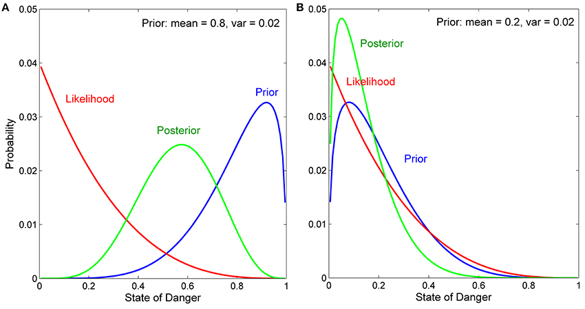
Figure A1. Effect of the mean of the prior distribution on Bayesian updating. Two individuals (A,B) are both exposed to the same experience, with the likelihood function indicated in red. The first individual (A) has a prior distribution with a high mean; the second individual (B) has a prior distribution with a low mean. When the likelihood function and the prior distribution contradict each other (A), the posterior distribution is displaced from the prior distribution. In contrast, when the likelihood function and the prior distribution are concordant (B), the posterior distribution is very similar to the prior distribution.

A second individual (Figure A1B) has a prior distribution with a low mean, indicating that when it is naïve, this individual estimates that the level of danger is more likely to be low than it is to be moderate to high. This individual is then exposed to the same experience (same likelihood function) as was the case for the individual in Figure A1A. However, in this case, the estimate of the state of danger provided by this individual's prior distribution is very similar to the estimate of the state of danger provided by the experience. As a result, its posterior distribution is very similar to its prior distribution. By extension, we would expect this individual's boldness score after the experience to be similar to its score when it was naïve.

This example illustrates a very general and very basic feature of Bayesian updating, namely that the effects of a given experience on estimates of the state of the world depend on the discrepancy between the prior distribution and the likelihood function (Courville et al., 2006). One can intuitively see that if a naïve individual believes that the world is a safe place, an extended period of time with no cues indicative of danger simply confirms its initial belief, and hence, has little or no effect on its belief that the world is safe. On the other hand, if a naïve individual believes that the world is dangerous, an extended period of time with no cues indicative of danger is a “surprise,” so this experience is more likely to change its estimate of danger.

A second important point is that the effect of a potentially informative experience on an individual's estimate of the state of the world also depends on the variance of its prior distribution (Figure A2). Consider a situation in which two individuals both have prior distributions with the same mean value (mean = 0.8). That is, when naïve, both of them estimate that the state of danger is relatively high. However, the variance of the first individual's prior distribution (Figure A2A) is much higher than the variance of the second individual's prior distribution (Figure A2B). Both individuals are then exposed to experience indicating that the level of danger is moderately low. In the case of the first individual, this experience leads to a reduction in its estimate of the level of danger, i.e., a posterior distribution shifted to the left of its prior distribution (Figure A2A). However, in the case of the second individual, the same experience has little effect on its estimate of danger; its posterior distribution is very similar to its prior distribution (Figure A2B). Thus, although both individuals would be expected to express the same high level of boldness when naïve, after the same experience, the first individual's level of boldness would increase, but the second individual's level of boldness would not change.

FIGURE A2

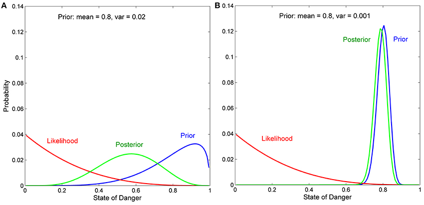
Figure A2. Effect of the variance of the prior distribution on Bayesian updating. Two individuals (A,B) are both exposed to the same experience, with the likelihood function indicated in red. Both individuals have prior distributions with the same mean, but the individual in (A) has a prior distribution with a high variance, whereas the individual in (B) has a prior distribution with a low variance. When variance of the prior is high (A), the posterior distribution is displaced from the prior distribution. However, when the variance of the prior is low (B), the posterior distribution is virtually the same as the prior distribution.

In this case, the intuitive explanation is that the variance of an individual's prior distribution indicates the confidence an individual has in its initial belief about the state of the world. If a naïve individual vaguely suspects that the world might be dangerous, experience indicating it is actually safe should alter its estimate of the state of the danger, and hence, its behavior. However, if a naïve individual firmly believes that the world is dangerous, that same experience should have little or no effect on either this belief or its behavior.