There is more to climate than the North Atlantic Oscillation: a new perspective from climate dynamics to explain the variability in population growth rates of a long-lived seabird

Introduction

The past two decades have produced a plethora of ecological studies that hinge on the North Atlantic Oscillation (NAO) as a proxy for “climate” (Sætre et al., 1999; Ottersen et al., 2001; Forchhammer et al., 2002; Stenseth et al., 2003; Durant et al., 2004; Sandvik et al., 2005, 2012; Dippner et al., 2014). This ubiquitous proxy usage may have led to the spread of a misconception of what NAO actually represents in an ecological context. Finding a statistical relationship without fully comprehending the underlying physics hinders the understanding of the climate-ecology interaction (Hallett et al., 2004; Stenseth and Mysterud, 2005). The point sometimes overlooked is that the NAO is just one of a number of modes of climate variability in the Northern Hemisphere (Barry and Carleton, 2001; Stenseth et al., 2003), as highlighted in Table 1. Thus, a better understanding of climate dynamics is critical before hinging on a proxy.

TABLE 1

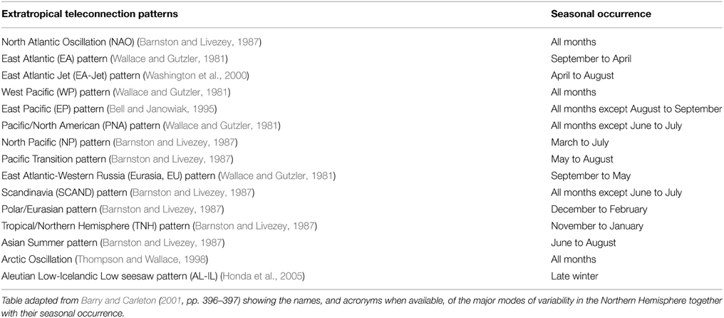
Table 1. Major teleconnection patterns in the Northern Hemisphere.

The NAO is defined as one of the leading modes of variability in the North Atlantic sector. It is characterized by an anomalous dipole of atmospheric pressure with centers over Iceland and Azores: a positive phase corresponds to a higher than normal subtropical high-pressure system and a deeper than normal low-pressure system called the Icelandic low (Hurrell, 1995; Barry and Carleton, 2001; Hurrell et al., 2003; Bader et al., 2011). The NAO could be considered as a manifestation of changes in the storm distribution: the cumulative effect of the storms and the associated changes in the storm track lead to the NAO signal (Mesquita et al., 2008, 2011). Nevertheless, the NAO is also influenced by other climatic processes, such as sea-ice changes in the Arctic and the Sea of Okhotsk in the North Pacific, and may shift its sign within a season (Bader et al., 2011; Mesquita et al., 2011). Even a single storm may have enough momentum to shift the NAO sign (Rivière and Orlanski, 2007) and the NAO is known to have a variable center of action (Zhang et al., 2008).

Indeed, with so many climatic features, it is no wonder the NAO “has recently become increasingly common to use” (Durant et al., 2004, p. 338). The use of the NAO as a “proxy,” without looking for other climatic clues, is implicitly based on the simplifying assumption that NAO is “climate variability.” This may, in the worst case scenario, lead to the erroneous conclusion that a certain ecological process is unrelated to climate, only because no relationship with NAO has been found. Furthermore, ther Sandvik et al. (2012) have shown that the relationship between the NAO and population growth rate of seabirds is highly variable, both within and across species. This alone does not mean that populations that do not co-vary with the NAO are unaffected by climate, however.

Furthermore, when studies use NAO without providing a clear climate dynamics framework behind its effect on ecology, they become pointless (Mysterud et al., 2000). Statistical results need to be supported by physical mechanisms. Finding that there is a relationship with a proxy without providing a physical mechanism for it may even make the validity of the relationship dubious. Correspondingly, Ottersen et al. (2001, p. 9), in an early review of the ecological effects of the NAO, warn against an overuse of a proxy without understanding its full implications: “Unless a mechanistically based explanation is provided, the veracity of any statistical NAO-ecology relationship will thus remain uncertain.” Moreover, relying on a specific proxy also makes it harder for ecologists to explain how atmospheric dynamics influence ecology (cf. Sydeman et al., 2014).

Thus, the objective of the present study is to illustrate standard statistical methods used in climatology to understand the connection between climate and ecological dynamics. Here, these methods will be applied to the population dynamics of the Common Guillemot Uria aalge, a long-lived seabird that breeds on Hornøya, a small island in northern Norway. Instead of starting with a proxy, this study will look one step before that, viz. finding what is affecting the species and where these climatic influences come from. Only afterwards, an appropriate climatic measure (or proxy) will be chosen. Our findings clearly demonstrate that there is more to climate than the NAO that impacts seabird populations.

Materials and Methods

Study Species, Study Area, and Data Collection

The Common Guillemot is a medium-sized (about 1000 g) seabird belonging to the auks (Alcidae). It is a colonial cliff-breeder with a circumpolar distribution in the boreo-low Arctic region. The Common Guillemot lays a single egg, which is incubated for 33 days on average. The chick is fed by both parents for 3 weeks, before it leaves the colony, still flightless, with its father. Birds start to breed when they are 5–7 years old, and annual adult survival is high (87–95%; Gaston and Jones, 1998). The Norwegian population amounts to approximately 15 000 breeding pairs, which represents a 90% reduction compared to the population size of the 1960s. The species is therefore listed as critically endangered in Norway (Kålås et al., 2010).

The fieldwork was carried out from 1980 to 2011 on Hornøya (70° 23′ N, 31° 9′ E), a 0.5 km² island in northeastern Norway. Annual counts of individual Common Guillemots on predefined monitoring plots were made by one of us (R.T.B.) late in the incubation period or during hatching. To minimize the day-to-day variation, five to ten counts were made on different days, and the mean number was used as an index of population size. The monitoring followed internationally standardized methods (Walsh et al., 1995). Successive annual estimates of the total population on Hornøya were based on a single, total count of 1900 individuals made in 1987 and the annual rates of change documented in the monitoring plots. See Barrett (1983, 2001) and Erikstad et al. (2013) for more details.

As can be seen from the population trajectory in Figure 1, there was a pronounced crash in population size from 1986 to 1987 (cf. Vader et al., 1990; and Erikstad et al., 2013). To estimate the yearly variation in population growth rate r, we used the variation in estimate of the total population size N in each census from 1 year to the next [r_t = ln (N_t/N_{t − 1})].

FIGURE 1

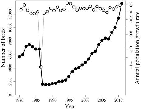
Figure 1. Dynamics of the Common Guillemot population on Hornøya, Northern Norway, from 1980 to 2011. Counts and estimates of numbers of breeding birds (filled circles, left-hand y-axis) and annual population growth rates r (open circles, right-hand y-axis). Figure adapted from and Erikstad et al. (2013).

Climate Datasets

Mean Sea Level Pressure Data

Mean sea level pressure (hereafter “MSLP”) from the European Centre for Medium-Range Weather Forecasts (ECMWF) Re-Analysis Interim Project (hereafter “ERA-Interim”) was used throughout this study (Berrisford et al., 2009; Dee et al., 2011). Re-analysis data “provide a multivariate, spatially complete, and coherent record of the global atmospheric circulation,” and the ERA-Interim reanalysis, particularly, is one of the most sophisticated gridded datasets at high-resolution at present (Dee et al., 2011, p. 554).

ERA-Interim data were created using the ECMWF Integrated Forecast System (IFS) model with fully coupled atmosphere, land surface, and ocean waves (Dee et al., 2011) together with the 4-dimensional variational assimilation (4D-Var) system (Courtier et al., 1994; Veerse and Thepaut, 1998; Dee et al., 2011). So, available observations from different sources (e.g.: satellite, station data) were assimilated into the model simulation, which allows for a product that is realistic (and in accordance with observational) data, with the advantage that it is on a three-dimensional lattice. In fact, rigorous quality control and experience from previous projects, such as ERA-40 (the precursor of ERA-Interim), have turned ERA-Interim into a state-of-the-art dataset for climate studies. ERA-Interim horizontal resolution is at T255 (nominally 0.703125°, or around 79 km) and it contains 60 vertical model levels, with the highest being at 0.1 hPa. The horizontal resolution in ERA-Interim (79 km) is higher than that for another reanalysis product (with resolution on the order of 250 km) used in recent ecological studies (Dippner et al., 2014).

Thus, in the present study, 6-hourly ERA-Interim MSLP data from 1980 to 2011 were used. The winter season, referred to here as DJF (December, January, and February) was retained, starting from December 1979. These seasonal data were then aggregated into yearly averages per grid point. So, from here on, we will refer to the MSLP as starting from 1980 (i.e.: December 1979, January and February 1980). This means, for instance, that when we discuss the year “1987” (outlier in the population growth rate data), we mean the winter 1986/87 (December 1986, January and February 1987) for the MSLP variable. This provides the equivalent of 32 years of data, which conforms to a 30-year period considered by the World Meteorological Organizations to be the minimum requirement for climate studies (Parry et al., 2007; Baddour, 2011).

Wind Data for Polar Low Tracking

High-resolution data are needed to identify and track polar lows due to their small-scale compared with synoptic-scale low-pressure systems. For this end, another high-resolution data product is needed. Here, wind data at the 850-hPa atmospheric level from the NCEP Climate Forecast System Reanalysis (NCEP-CFSR) data were used (Saha et al., 2010, 2013). The NCEP-CFSR is a state-of-the-art reanalysis fully coupled product at the spectral T574 horizontal resolution (~27 km) and 64 vertical levels, which is arguably one of the most advanced products at high-resolution to date. The importance of reanalysis data to climatologists was also expressed in Saha et al. (2010 p. 1015), “The general purpose of conducting reanalysis is to produce multiyear global state-of-the-art gridded representations of atmospheric states.” Thus, the combination of an advanced storm-tracking algorithm (described below) with high-resolution advanced reanalysis dataset makes the result of this study unique.

Differently from ERA-Interim, the NCEP-CFSR was based on a fully coupled model system, the Climate Forecast System version 2 model (CFSv2), combined with an advanced data assimilation system (Saha et al., 2013); but like the ERA-Interim, NCEP-CFRS made use of the same observations from a number of sources in its assimilation system. These sources come from satellite data, aircraft and upper air balloon observations, as well as surface datasets.

Statistical Methods

Point Correlation Maps

Point correlation maps allow for the organization of large-data information and make it possible to identify climatic modes of variability (Wilks, 2011, pp. 67–70). This technique has been used in climate science for several decades. In fact, Wilks' (2011, p. 69) figure 3.28 shows the reproduction of a figure taken from the Norwegian climatologist Bjerknes (1969, p. 169). This figure illustrates that by using the method of point correlation for annual surface pressures around the globe with those in Djakarta, Indonesia, Bjerknes was able to identify a strong negative correlation with Easter Island, which reflects the atmospheric component of the El Niño-Southern Oscillation (ENSO). This is an example of a teleconnection pattern, that is, a remote phenomenon can affect other regions around the world (Glanz et al., 2009). It is interesting to note that Bjerknes' figure was also a reproduction of the earlier work of Berlage (1957), which exemplifies that this technique has been around for a long time as a means of understanding climate dynamics.

In this study, point correlation maps were created using the sample cross correlation at lag 0. Other lags could have been shown, but Sandvik et al. (2005 p. 823) find that the NAO has the highest correlation with the survival of Common Guillemot at lag 0 and here we test this effect. So, let X_{i, j} be the vector of MSLP for latitude-longitude coordinate points i and j in the ERA-Interim grid, and Y be the vector of population growth rates for Common Guillemot. Thus, the sample correlation is determined as:

${\rho }_{i,j}=\frac{Cov(X_{i,j},Y)}{\sqrt{Var(X_{i,j})Var(Y)}}$

where ρ_{i, j} is the correlation coefficient at location i and j. Cov and Var represent the covariance and variance, respectively. The statistical significance of the correlation coefficient can be determined using Student's t-test (von Storch and Zwiers, 2002, pp. 77–78).

Point Regression Maps

Similarly, point regression maps can be created to aid the identification of hotspots where the predictor variable (e.g.: MSLP in this case) and the response variable (e.g.: population growth rate) are linearly related. These maps can be created through the least squares method, which is used to obtain meaningful information about the dependency relationships between variables (Draper and Smith, 1998). Also, the creation of such maps is often used in climatology and can provide further insights on how remote processes can affect other regions around a hemisphere or the globe (Bader et al., 2011; Mesquita et al., 2011).

Regression maps are created by plotting the regression coefficient, that is, the slope (β₁) of the linear regression equation:

$Y_{k;i,j}={\beta }_0+{\beta }_1{X}_{k;i,j}+{\epsilon }_{k;i,j}$

where Y_k;i,j, represents the k-th element of the response variable at location i and j, β₀, and β₁ are the intercept and the slope parameters, respectively; and ε is the error variable. The slope is estimated β₁ as follows (Draper and Smith, 1998):

${\beta }_1=\frac{{\displaystyle \sum (X_{k;i,j}-{\overline{X}}_{i,j})(Y_{k;i,j}-{\overline{Y}}_{i,j})}}{{\displaystyle \sum {(X_{k;i,j}-{\overline{X}}_{i,j})}^2}}$

where the overbar represents the mean values of X and Y at location i, j on the lattice. A t-test was used for significance for each grid point, which can then be overlayed on the map. A significance level of 0.1 was used to identify potential regions that can later be combined to construct an index.

Composite Analysis

Composite analysis is a well-known technique in climatology, which is used to construct climatic states that are typical (von Storch and Zwiers, 2002, p. 378). In order to illustrate the definition of composite analyses, we adapt the definition given in von Storch and Zwiers (2002, p. 378) as follows. Let z be a univariate index and M be the vector of the mean sea level pressure variable at a certain grid point. The composite is defined as:

$M_{\Theta }=\epsilon (M_t|z_tϵ\Theta )$

where Θ represents sets of the index z and t represents time. The expectation of the composite is generally estimated as:

$M_{\Theta }=\frac{1}{k}{\displaystyle \sum _{s=1}^k{M}_{t_s}}$

for the observing times t₁, …, t_k for which z_t ∈ Θ. In this study, composites were made for two sets: MSLP for the 5 years with the highest population growth rates (Θ_h) and MSLP for the 5 years with the lowest population growth rates (Θ_l). We estimate the difference between M_Θh − M_Θl applied to each grid point on the globe. In more general terms, composite analysis is the difference between selected states. For example, the difference between the mean of MSLP maps corresponding to years when the population growth rate of Common Guillemot is above/below a certain threshold with the mean of MSLP maps for years when the population growth rate is above/below a certain threshold average. This technique provides insights into atmospheric patterns that are more common for specific states of the population growth rate.

Storm Tracking Algorithm

In order to understand the 1987 crash, the storm-tracking algorithm TRACK, developed by Hodges (1995, 1999), was used. TRACK is a computer algorithm, which has been applied in several storm-related studies (Mesquita et al., 2008, 2011; Bader et al., 2011; Zappa et al., 2014). Storms were identified in relative vorticity maps at the 850-hPa atmospheric level and were tracked temporally through a cost function. Relative vorticity represents the curl of the wind and how much it spins. It is determined from the u (west-east direction) and v (north-south direction) components of the wind, and is defined as (Holton, 2004, p.92):

$\zeta =\frac{\partial v}{\partial x}-\frac{\partial u}{\partial y}$

For the present study, polar lows, which are short-lived storms with a radius on the order of 100–500 km and surface wind speeds above 15 m s⁻¹, were tracked using the criteria detailed in Zappa et al. (2014, p. 2603) with NCEP-CFSR (described above) as the input data.

Population Modeling

As a test of the utility of the different climatic indices in explaining Common Guillemot population dynamics, these indices were used as covariates in stochastic population models. Different models were compared using their AIC_C (Akaike Information Criterion corrected for small sample size). All estimates are provided as means alongside their 95% confidence intervals.

Population dynamics of the Common Guillemot population on Hornøya were density-independent, as evidenced by the absence of a negative correlation between annual growth rates r_t and population sizes N_t (correlation coefficient R = +0.0005 ± 0.3664, p = 0.998), and the fact that the AIC_C of the density-dependent (logistic) population model exceeded that of the density-independent (Brownian) model by 2.48 units. The model used thus had the form:

$\ln N_{t+1}=\ln N_t+\overline{r}-\frac{1}{2}{\sigma }_{\text{d}}^2{N}_t^{-1}+{\displaystyle \sum {\beta }_i}{X}_{i,t}+{\epsilon }_t$

where β_i represents the slope of the ith environmental covariate X_i; ε, environmental noise, i.e., an independent variable with zero mean and variance σ²_e; N_t, population size in year t; r, long-term intrinsic population growth rate; σ²_d, demographic variance; X_{i, t}, environmental covariate i in year t. The parameters β_i, r, and σ²_e were estimated using maximum likelihood (for details, see Sæther et al., 2009; Sandvik et al., 2014), while σ²_d was assumed to be 0.1, which is a realistic value for long-lived birds (Lande et al., 2003). To ensure that the latter assumption did not critically affect the results, different values of σ²_d were tested; varying σ²_d tenfold (0.01–1) changed the estimate of β by less than 2%. As the crash from 1986 to 1987 represented an influential outlier, population dynamics were analyzed with and without the population count for the year of 1986 included.

Computations were carried out through: (a) the R environment (R Development Core Team, 2013); (b) NCL (The NCAR Command Language, 2014¹); (c) CDO, the Climate Data Operators (Schulzweida, 2013), and (d) the coupled general circulation model MPI-ESM1 (Giorgetta et al., 2013).

Results

Correlation Maps

The point correlation between winter MSLP and the population growth rate variable are shown in Figure 2. Colors in red represent areas where the correlation is positive, meaning that high values of pressure in winter are associated with high values of the population growth rate that year (i.e., from the previous to next breeding season). An increase in pressure is related to a high-pressure system, which can promote cold air activity in winter, and a decrease in storm activity. Colors in blue are related to negative correlation between the variables. So in this case, a decrease in the values of winter pressure is associated with high values of the population growth rate. A decrease in pressure is related to low-pressure systems, which bring moisture and heat from lower to higher latitudes that create milder conditions in winter.

FIGURE 2

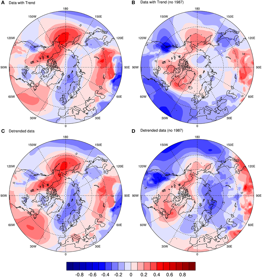
Figure 2. Point correlation between mean sea level pressure (MSLP) and guillemot population growth rate (r) based on the period from 1980 to 2011. The four plots display the correlation coefficient calculated as: (A) MSLP and raw r; (B) MSLP and r with 1987 removed from both series; (C) MSLP and detrended r; (D) MSLP and detrended r with 1987 removed from both series.

Figure 2A shows the correlation with the raw population data (includes the trend). It shows a clear dipole structure in the Arctic, as well as a wave-like propagation of positive-negative centers of correlation in mid-latitudes. The figure shows little or no resemblance to the NAO pattern in the Atlantic, but shows some resemblance, although shifted in center of action, to the Arctic Oscillation (Thompson and Wallace, 1998). It is, however, more similar to the Aleutian Low and Icelandic Low (AL-IL) seesaw pattern observed in later winter, another atmospheric mode of variability, which results in a dipole in the Arctic. The AL-IL is also the dominant pattern in late winter and it has consequences for climate in the surrounding regions (Honda et al., 2005).

The correlation with the detrended population data (Figure 2C) is quite similar in structure to that in Figure 2A. In fact, this pattern suggests that the trend in the population growth rate does not account for the seesaw-like pattern; it is a feature of another aspect of the population data. In order to investigate this, Figure 2B shows the data with trend, but removing the outlier in 1987 (i.e.: winter 1986/87 for MSLP; 1987 for r). Here, the features look very different indeed. The low pressure over where the colony is located is still there, but the seesaw pattern is much weaker. Also, for mid-latitudes, there is an increase in negative correlation.

Finally, the data with no trend together with the removal of the year 1987 is shown in Figure 2D. The pattern is similar to that in Figure 2B, but it has much stronger correlation features, especially over the Barents Sea, where the colony is located. The features in the mid-latitude Pacific and Atlantic are also different compared with Figure 2B, with almost an opposite effect. The pattern in the Atlantic sector resembles another mode of variability called the Barents Oscillation (Chen et al., 2013), an anomalous atmospheric oscillation associated with flow over the Nordic Seas, although with a shifted center of action.

Thus, 1987 is indeed an outlier, which seems to be related to a strong seesaw pattern in the Arctic. The main feature of the four figures is the low-pressure system over the Barents Sea and Pacific sector, as well as the high pressure over the Bering Sea. Both the outlier and the low-pressure system over the Barents Sea are investigated further in subsequent sections. But first, we investigate the aforementioned features through the use of point regression.

Regression Maps

Regression maps are given in Figure 3. Similar to correlation maps, the colors indicate regions of high (red) or low pressure (blue) associated with the population growth rate. Looking at the significant regions across Figures 3A–D, one can see some consistent patterns, such as the Bering Sea, Pacific Ocean and northwestern parts of North America, as well as the Barents Sea. If we focus on the latter, that is, the region where the colony is located, we observe that the regression with the detrended data without 1987 is significant. Thus, the trend and the outlier seem to mask the significance, showing that the pattern over the Barents Sea is the true underlying process (or signal) associated between pressure and population growth rate.

FIGURE 3

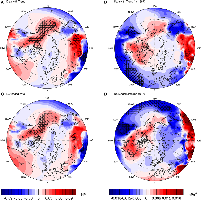
Figure 3. Point linear regression coefficients between MSLP and guillemot population growth rate (r) based on the period 1980–2011. Each plot shows the regression coefficient between: (A) MSLP and raw r; (B) MSLP and r with 1987 removed from both series; (C) MSLP and detrended r; (D) MSLP and detrended r with 1987 removed from both series. Crosses represent regions where the p-value of a t-test statistic is less than 0.10. Units: population growth rate/hPa.

Regression maps are very useful in identifying “hotspots” of regions that have potential in explaining the association between the dependent and explanatory variables. Here they show, as pointed out before, that the pattern of the NAO does not emerge in Figures 2, 3. For instance, if a consistent dipole pattern between a region around Iceland and the Azores emerged, one would then relate it to the NAO. But this is not the case here.

Composite Maps

In Figure 4, composite plots of MSLP are displayed for the 5 years with the highest (i.e.: 1995, 1996, 1982, 2011, 2002) and the lowest (i.e.: 1987, 1985, 1984, 1988, 2007) detrended population growth rates. These plots provide further support to the robustness of the findings in Figures 2, 3, and are commonly used in climate studies. Figures 4A,B, show that the general patterns seem similar, however, the absolute values of the contour lines in the Pacific and Atlantic basin, as well as the distance between contours are different. The latter refers to the strength of the pressure gradient and provides an indication of the relative strength of the wind. So, in years with negative population growth rates, there is an intensification of the pressure gradient in both ocean basins compared to years with positive population growth rates.

FIGURE 4

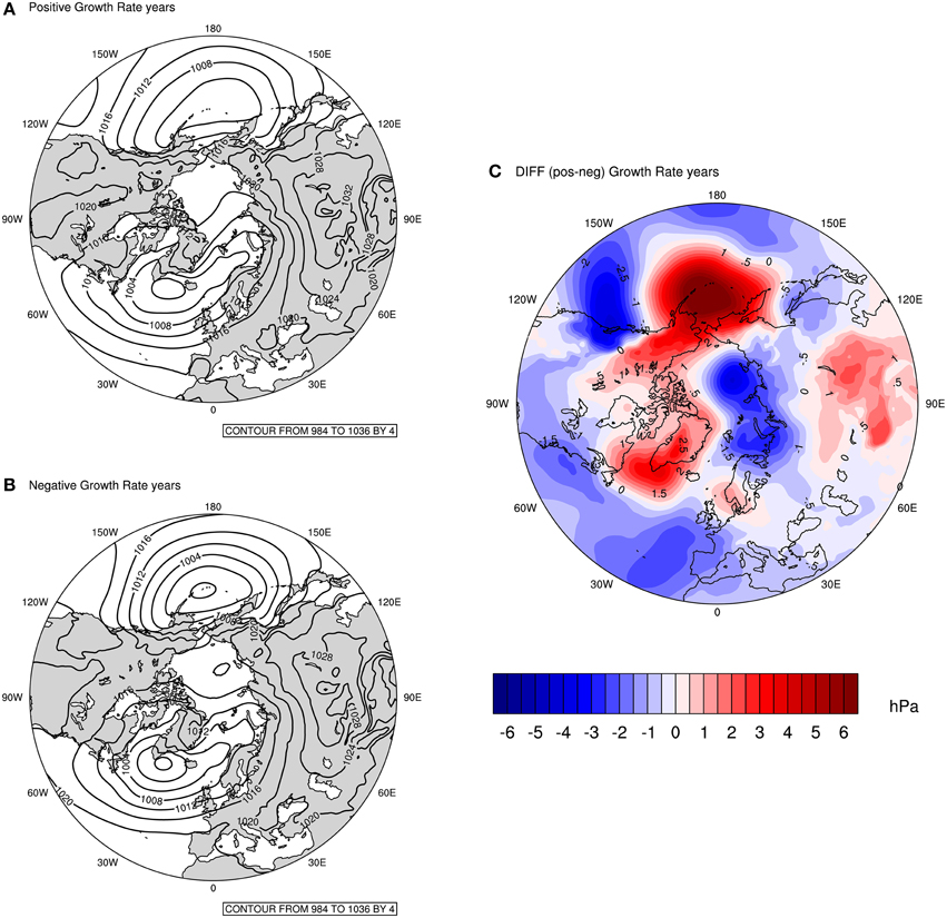
Figure 4. MSLP Composite for: (A) Five years with the highest positive guillemot population growth rates (top left); (B) Five years with the highest negative population growth rates (bottom left); (C) Difference between 5 years with highest positive and 5 years with highest negative population growth rates. Units: hPa.

The difference plot (Figure 4C) shows the difference between the MSLP for years with positive and negative population growth rates (i.e.: Figure A minus Figure B). Here, there is a striking similarity with the features observed in Figures 2, 3; more importantly, the dipole pattern in the Arctic between the Barents and Bering seas are evident. Thus, the fact that the feature observed in the Barents Sea is clearly seen in this composite confirms that the population growth rate is associated with the low-pressure system over the Barents region during winter. The dynamics behind this system will be explained further on.

Analysis of the Outlier

Composite Analysis

Composite analysis has also been used to understand what the atmospheric features of 1987 were and how anomalous it was with respect to different climate baselines. Figure 5 displays these composite maps. Figure 5A shows the MSLP configuration for the winter 1986/1987. Compared with Figure 4, the isobars (lines of same pressure level) seem to be much tighter both in the Pacific and the Atlantic basins. In fact, if one would rank Figures 4A,B, 5A based on the spacing of the isobars, Figure 5A would feature as the one with the least spacing between then. This is a first indication that the 1986/87 winter had an atmospheric feature that was stronger than that of the MSLP for the years with the lowest negative population growth rates.

FIGURE 5

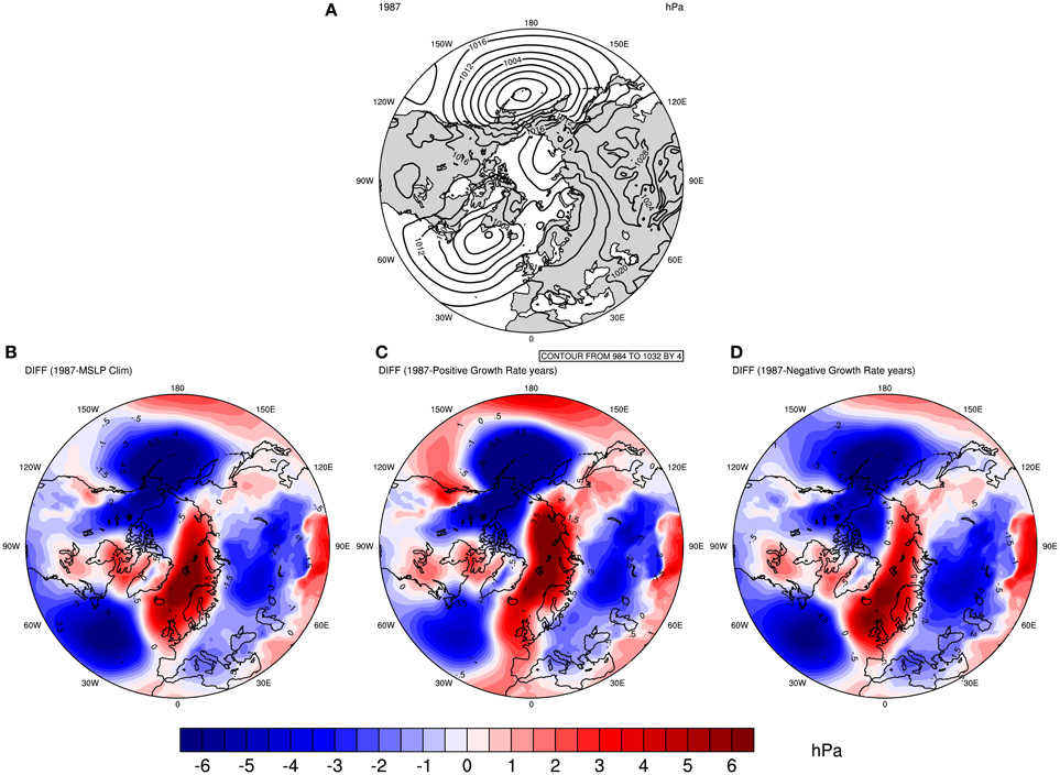
Figure 5. Comparison between MSLP in 1987 with different baselines. (A) The MSLP in 1987. The bottom figures represent the MSLP in 1987 minus the MSLP in the following periods: (B) mean of 1980–2011; (B,C) Five years with the highest guillemot positive population growth rates of the detrended dataset; (C,D) Five years with the lowest negative population growth rates of the detrended dataset excluding year 1987.

The bottom panel in Figure 5 shows anomaly plots, defined as the difference between MSLP for winter 1986/87 minus different winter baselines (from left to right): the mean of 1980 to 2011; the 5 years with the highest positive population growth rates in the detrended dataset (i.e.: 1985, 1984, 1988, 1998, 2007); and the 5 years with the lowest negative population growth rates in the detrended dataset excluding year 1987 (i.e.: 1982, 1992, 1995, 1996, 2011). These figures show a major correspondence with those in Figures 2–4, but with the colors shifted. This correspondence is especially seen for the Barents–Bering dipole pattern. The red color observed over the Barents Sea means that 1987 had an anomalous high-pressure system over the region, and as considered in the previous figures, a high-pressure system during winter in the Barents Sea is associated with a low population growth rate for that year.

Thus, the winter of 1986/1987 features as having an anomalous atmospheric configuration compared with different baselines. It had a major zone of high-pressure system, the so-called atmospheric blocking, over the Barents Sea. The latter feature was anomalous throughout the climatology of the region for the period considered here (1980–2011).

Effect of Local Weather

The results in the previous subsection indicate that the winter 1986/87 was indeed an outlier when it comes to the climatological conditions in the Barents Sea. It is therefore useful to look at the weather conditions that winter. Polar lows are a common feature in that region, which bring anomalously cold air from the pole, can have relative strength of a violent tropical storm (Nordeng and Rasmussen, 1992) and have damaging effects at the surface, such as icing (Icing implies the deposition and formation of ice on surfaces). Figure 6 shows mesocyclones, which are medium-sized storms, and polar lows in the North Atlantic and Barents Sea. The figure shows at least four polar lows crossing the central Barents Sea, which is the area where Common Guillemots from Hornøya spend the entire winter, according to ring recoveries (Barrett and Golovkin, 2000) and 3 years of geolocator data (Erikstad et al., unpubl. data). These polar lows were quite strong systems, as indicated by the vorticity, which represents how much the wind spins, with values higher than about 9 × 10⁻⁵s⁻¹. This suggests that through elevated thermoregulatory costs (due to low temperatures) and periodic difficulties in finding food (through high winds) the polar lows that winter could have increased the mortality of Common Guillemot. Indeed, many corpses of emaciated Common Guillemots were found washed ashore in Finnmark that winter (Vader et al., 1990).

FIGURE 6

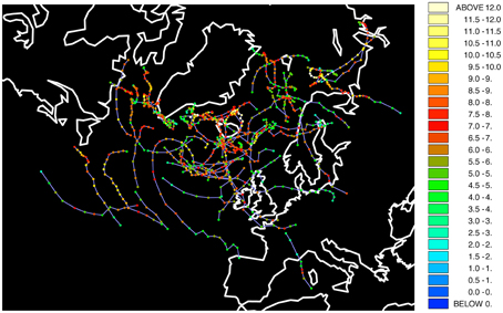
Figure 6. Mesocyclones and polar lows in winter 1986/1987 from NCEP-CFSR data and tracked through Hodges' TRACK algorithm. Colors represent strength as based on vorticity. Units: 10⁻⁵ s⁻¹.

Building Proxies

Four regions were selected for the construction of climatic indices, or proxies (Figure 7). These were selected based on the correlation and regression patterns discussed previously. Note that other regions could have been chosen, but here we illustrate how a useful climate “proxy” could be created and used in ecology. The regions are as follows: Barents, “BAR” (65-75N, 30-75E), north-eastern North America, “NEA” (48-60N, 46-63W), Alaska, “AKA” (63-70N, 155-170W), and Pacific, “PCF” (30-43N, 140-160W). The indices were constructed by first calculating the DJF MSLP average of each region and then making different combinations of similar polarity (i.e.: combining regions with positive correlation against negative correlation regions). These indices were then normalized. They are: IDX1 (BAR−NEA), IDX2 (PCF−AKA), and IDX3 [(PCF+BAR)−(NEA+AKA)].

FIGURE 7

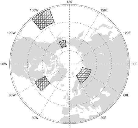
Figure 7. Regions selected for the MSLP-based index.

Testing the Proxies

As a test of the utility of the indices described above, these indices, as well as the NAO index, were used as covariates in stochastic population models. When detrended, the two indices IDX2 and IDX3 improve the null population model (without covariates) by more than two AIC_C units (Table 2). Both models are thus equally well supported, and considerably better so than the null model. Each of these two covariates explains 15% of the population dynamics. IDX2 and IDX3 with trends retained, as well as a pure trend model, are much poorer, in that they are roughly equally well supported as the null model (Table 2). NAO and IDX1 do not improve the null model, and explain less than 5% of the population dynamics. The finding that the NAO cannot physically explain the population dynamics of the Common Guillemot, is in accordance with the observation that NAO does not appear to be a mode of variability identified in Figures 2–5, either.

TABLE 2

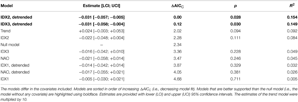
Table 2. Stochastic population models of the Common Guillemot population on Hornøya.

Models with two or more covariates did not improve upon the best models with one covariate (results not shown). Lagged covariates performed more poorly than their unlagged counterparts and/or the null model in all cases (time lags of 1–3 years were considered; results not shown).

The above results are based on population dynamics with the crash year removed. Even when 1986 is retained in the population time series, however, a detrended IDX3 is able to significantly improve upon the null population model (AIC_C 2.5 units lower than null model, p = 0.026, R² = 0.148). The remaining indices (IDX1, IDX2, NAO) do not differ from the null model in this case (results not shown).

Discussion

Although the analysis of the population growth rate of Common Guillemot under classical climatological methods focused mainly on the mean sea level pressure variable, it addressed the main objective of this paper, that is, to highlight the need to understand the climate dynamics behind an ecological variable before constructing a so-called “proxy.” In what follows, we present a discussion of the main results and propose a model to explain the atmospheric dynamical effect on the population growth rate variable.

The Hornøya population of the Common Guillemot, a species that is classified as “critically endangered” according to the Norwegian Red List (Kålås et al., 2010), declined by 80% in winter 1986/87 (Vader et al., 1990; and Erikstad et al., 2013). The year 1987 was indeed an extreme event, as could be confirmed by the anomalous high-pressure system over the Barents Sea, where the colony is located. It has been previously shown that the crash of Common Guillemot was related to low fish stocks (Vader et al., 1990; and Erikstad et al., 2013), but it is possible that this situation was aggravated by (or even causally related to) the overlaying atmospheric condition in the winter 1986/87. From the clear and robust pressure system over the Barents region, as a response from the Pacific Ocean teleconnectivity, we could hypothesize that biotic responses (fish and/or birds) might have been forced by the atmospheric conditions over the Barents Sea. Note also that, the response in the Barents Sea is also forced through changes in sea ice, as shown in Figure 8. This highlights the importance of considering the climate system as a whole in the understanding of changes in ecological variables (cf. Sydeman et al., 2006).

FIGURE 8

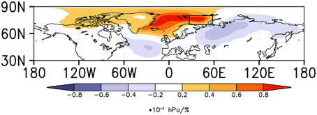
Figure 8. Surface pressure regressed on sea-ice concentration in the Barents Sea. Sea-ice time series selected from the region indicated by the box. The data are based on the Coupled Model Intercomparison Project through the Max Planck Institute Earth System Model, CMIP5 MPI-ESM, control integration. Units: Coloring shows the change in hPa per one percent sea-ice concentration change multiplied by 10.

There is mixed evidence for the relevance of NAO in ecology. NAO can explain variation in some different ecological variables in some species, but not in others (e.g.: Sætre et al., 1999; Forchhammer et al., 2002; Durant et al., 2004; Sandvik et al., 2005; Sæther et al., 2009; Dippner et al., 2014; Sandvik et al., 2014). These studies and others illustrate the fact that NAO can be highly relevant for some variables and species; but an association may not mean causation. More is needed to assess NAO's usefulness, in this case, by finding a climate dynamics link to explain the association. The latter is clearly expressed in Forchhammer et al. (2002, p. 1002) when discussing the impact of climate perturbations on arrival on breeding grounds and later survival and reproduction: “the timing of migration must be adapted ultimately to large-scale atmospheric systems.” This large-scale referred to by the authors is the idea of looking at the bigger picture, before making a choice of an index to explain the variability. Therefore, looking for the dynamics first, before selecting an index, is here suggested as a more promising approach.

Sandvik et al. (2005, p. 826) also recognize that: “causal pathways of these interactions are not easily identified. The NAO is defined as a temporal fluctuation of sea level pressure anomalies… and can as such hardly be said to be the cause of any of these responses. Rather it is convenient to treat the NAO as a “proxy” for different climatic processes… A full understanding of any climate-related response requires that one identifies the factors that cause it.” The latter points to the need to look at the spatial contribution first to identify what affects the variability. In the present study, the variability explained by the NAO is not robust and does not appear in the spatial analysis of the relationship between MSLP and population growth rate, as concluded from the analysis of a long time series of the population growth rate of Common Guillemots. The local effects in the Barents Sea, which include the atmospheric forcing, mediated via teleconnectivity as found in this study, and the SST effects on the food web may act to affect the food web. This is also in line with the fact that there are positive correlations between SST and herring recruitment and stock biomass, which are relevant for Common Guillemot (Erikstad et al., 2013).

In the light of the results found in the present paper, and the discussions of previous scientific work, we propose the following mechanism to explain the variability in the population growth rate of Common Guillemot:

• An anomalous low-pressure over the Barents Sea during winter, forced via teleconnectivity through the Pacific and local sea-ice changes, leads to the increase of moisture and heat brought by storm tracks into the region. This forces the SST locally and leads to warmer conditions—favorable conditions for Common Guillemot.

• An anomalous high-pressure over the Barents Sea during winter, forced via teleconnectivity through the Pacific and local sea-ice changes, leads to blocking of storm tracks and loss of long-wave radiation from the surface to space. This leads to cold conditions both in the atmosphere and ocean—unfavorable conditions for Common Guillemot.

Based on this model, the anomalous year of 1987 can also be explained. During the 1986/87 winter, the high-pressure was more anomalous than any other years in the study period. This led to extremely unfavorable conditions to Common Guillemot. With lack of food and increased energetic costs, these seabirds were at a great disadvantage. Any other external factor might be enough to cause a crash, such as the polar lows that brought even colder air from the pole and high winds into the region.

We conclude that the role played by the Pacific as well as the Barents Sea is significant. It might indicate that the changes observed in the Barents Sea, where the colony is located, is triggered by a teleconnection from the Pacific via Alaska or via the north-east North America regions; these changes are also influenced by local changes in sea-ice.

Conclusion

The ubiquitous use of the NAO as a “proxy” in ecology and the search for alternative means of explaining variability have been analyzed in this research work. Although the NAO can explain the climate variability in the Atlantic sector, it is not the only teleconnection index available, and there needs to be a physical basis for the use of the NAO. So, the NAO as a “proxy” on its own should be used with caution. Also, before a decision is made on any proxies, one needs to see the bigger picture of what the possible climatic mechanisms are and how they can influence an ecological process.

Here, in search of such mechanisms, classical methods used in climatology to study climatic interactions were illustrated to study population growth rate of Common Guillemot: spatial maps of correlation and regression, compositing and a tracking algorithm to search for polar lows. We have used one climate covariate at the surface level for the analysis (i.e.: MSLP), and it has revealed an important climate mechanism at the Barents Sea. MSLP is just one of many other variables that could have been explored, such as: surface temperature, sea ice, temperature at different altitudes, geopotential height, precipitation, relative humidity, among others, to create a larger picture of the climate system and the interaction with the species studied here. Also, these variables could have been combined into a multivariate study and other advanced methods could have been used to explore their relationship. Thus, the present study illustrates the richness of information one gains through looking at ecology using the perspective that there is more to climate than the NAO.

Also, a possible physical mechanism was then proposed from the analysis, which linked teleconnectivity interaction via the Pacific into the Barents Sea, as well as interaction with sea ice changes in the Barents Sea region. An anomalous winter low-pressure system over the Barents Sea is associated with higher population growth rates, compared with years when an anomalous high pressure system is present: it creates warmer conditions brought by synoptic-scale storm track into the region. The opposite is true in anomalous winters with high-pressure system over the Barents Sea. The crash in 1987 could be explained by the extreme conditions of the severe anomalous high-pressure system over the region and the presence of polar lows.

One might ask if the techniques presented here apply to other species or variables. The answer is yes, but each species or variables would need to be analyzed on a case-to-case basis or through the use of multiple regression techniques. The latter is the subject of the next phase of this research work, where the idea of synchronization with different species and teleconnectivity will be explored. In doing so, other climate variables will also be addressed, such as sea surface temperature and geopotential height—in order to provide more insights into the dynamics of climate interactions and seabirds.

Overall, this research work has pointed to the importance of looking at what the data are telling in connection with climate-related variables, instead of starting from on a specific “proxy.” Only after the larger picture is obtained, can one narrow down existing modes of variability and/or create indices based on the response from the data. Thus, instead of looking at the data given the “proxy” (or mode of variability), [Data|Mode], one should explore the idea of looking at the climatic forcing given the data, [Forcing|Data], in search of modes of variability. Future work should address what is happening in the Pacific that triggers a wave-like pattern of teleconnectivity, as well as an integrated approach to understanding how climate affects seabirds, by looking at the role of climate forcing (ocean and atmosphere) on predator and prey in a multivariate fashion.

Author Contributions

M.d.S.M wrote the manuscript, devised the climate analyses, concept and design of the research work; K.E.E. provided data, figure and participated in the conception and design of the work; H.S. conducted the population modeling, wrote part of the manuscript and critically evaluated the work; R.T.B. provided ecological expertise, data information and critically evaluated the work; T.K.R. contributed with ecological expertise, discussions on the climate mechanism and critically evaluated the work; T.A.-N. provided ecological expertise, helped draft the work and critically evaluated it; K.I.H. conducted the polar low analysis, provided figure, critically evaluated the work and helped with climatological methods; J.B. helped draft the work, critically evaluated it, provided a figure and helped with climatological methods.

Conflict of Interest Statement

The authors declare that the research was conducted in the absence of any commercial or financial relationships that could be construed as a potential conflict of interest.

Acknowledgments

We would like to thank Fram Centre, NINA and the Centre for Biodiversity Conservation Dynamics for providing funding to this research. We also thank Giuseppe Zappa (University of Reading) for producing the tracks of the polar lows and Marine Ecology Progress series for the permission to reproduce Figure 1. We are very grateful to the National Seabird Monitoring Programme, which is funded by the Norwegian Environment Agency, for organizing the monitoring of Common Guillemots on Hornøya island.

Footnotes

1. ^The NCAR Command Language. (2014). Boulder, Colorado: UCAR/NCAR/CISL/VETS. Available online at: http://dx.doi.org/10.5065/D6WD3XH5

References

Baddour, O. (2011). Climate Normals. Denver, CO: World Meteorological Organization. Available online at: https://www.wmo.int/pages/prog/wcp/ccl/mg/documents/mg2011/CCl-MG-2011-Doc_10_climatenormals1.pdf (Accessed July 25, 2014).

Bader, J., Mesquita, M. D. S., Hodges, K. I., Keenlyside, N., Østerhus, S., and Miles, M. (2011). A review on Northern Hemisphere sea-ice, storminess and the North Atlantic Oscillation: observations and projected changes. Atmospheric Res. 101, 809–834. doi: 10.1016/j.atmosres.2011.04.007

CrossRef Full Text | Google Scholar

Barnston, A. G., and Livezey, R. E. (1987). Classification, seasonality and persistence of low-frequency atmospheric circulation patterns. Mon. Weather Rev. 115, 1083–1126.

Google Scholar

Barrett, R. T. (1983). Seabird Research on Hornøya, East Finnmark with Notes from Nordland, Troms and W. Finnmark 1980–1983. Tromsø museum: unpubl. rep.

Barrett, R. T. (2001). Monitoring the Atlantic puffin Fratercula arctica, common guillemot Uria aalge and black-legged kittiwake Rissa tridactyla breeding populations on Hornøya, northeast Norway, 1980–2000. Fauna Nor. 21, 1–10.

Barrett, R. T., and Golovkin, A. N. (2000). “Common guillemot Uria aalge,” in The Status of Marine Birds Breeding in the Barents Sea Region, eds T. Anker-Nilssen, V. Bakken, H. Strøm, A. N. Golovkin, V. V. Bianki, and I. P. Tatarinkova (Tromsø: Norsk Polarinst. Rapp.), 114–118.

Barry, R. G., and Carleton, A. M. (2001). Synoptic and Dynamic Climatology. London: Routledge. doi: 10.4324/9780203218181

CrossRef Full Text | Google Scholar

Bell, G. D., and Janowiak, J. E. (1995). Atmospheric circulation associated with the midwest floods of 1993. Bull. Am. Meteorol. Soc. 76, 681–695.

Google Scholar

Berlage, H. P. (1957). Fluctuations of the General Atmospheric Circulation of more than One Year, their Nature and Prognostic Value. De Bilt: Koninklijk Nederlands Meteorologisch Instituut.

Berrisford, P., Dee, D., Fielding, K., Fuentes, M., Kallberg, P., Kobayashi, S., et al. (2009). The ERA-Interim Archive. Reading: European Centre for Medium-Range Weather Forecasts Available online at: http://old.ecmwf.int/publications/library/ecpublications/_pdf/era/era_report_series/RS_1.pdf

Bjerknes, J. (1969). Atmospheric teleconnections from the Equatorial Pacific. Mon. Weather Rev. 97, 163–172.

Google Scholar

Chen, H. W., Zhang, Q., Körnich, H., and Chen, D. (2013). A robust mode of climate variability in the Arctic: the Barents Oscillation. Geophys. Res. Lett. 40, 2856–2861. doi: 10.1002/grl.50551

CrossRef Full Text | Google Scholar

Courtier, P., Thépaut, J.-N., and Hollingsworth, A. (1994). A strategy for operational implementation of 4D-Var, using an incremental approach. Q. J. R. Meteorol. Soc. 120, 1367–1387. doi: 10.1002/qj.49712051912

CrossRef Full Text | Google Scholar

Dee, D. P., Uppala, S. M., Simmons, A. J., Berrisford, P., Poli, P., Kobayashi, S., et al. (2011). The ERA-Interim reanalysis: configuration and performance of the data assimilation system. Q. J. R. Meteorol. Soc. 137, 553–597. doi: 10.1002/qj.828

CrossRef Full Text | Google Scholar

Dippner, J. W., Möller, C., and Kröncke, I. (2014). Loss of persistence of the North Atlantic Oscillation and its biological implication. Front. Ecol. Evol. 2:57. doi: 10.3389/fevo.2014.00057

PubMed Abstract | Full Text | CrossRef Full Text | Google Scholar

Draper, N. R., and Smith, H. (1998). Applied Regression Analysis, 3rd Edn. Hoboken, NJ: John Wiley & Sons. doi: 10.1002/9781118625590

CrossRef Full Text | Google Scholar

Durant, J. M., Anker-Nilssen, T., Hjermann, D. Ø., and Stenseth, N. C. (2004). Regime shifts in the breeding of an Atlantic puffin population. Ecol. Lett. 7, 388–394. doi: 10.1111/j.1461-0248.2004.00588.x

CrossRef Full Text | Google Scholar

Erikstad, K. E., Reiertsen, T. K., Barrett, R. T., Vikebø, F., and Sandvik, H. (2013). Seabird-fish interactions: the fall and rise of a common guillemot Uria aalge population. Mar. Ecol. Prog. Ser. 475, 267–276. doi: 10.3354/meps10084

CrossRef Full Text | Google Scholar

Forchhammer, M. C., Post, E., and Stenseth, N. C. (2002). North Atlantic Oscillation timing of long- and short-distance migration. J. Anim. Ecol. 71, 1002–1014. doi: 10.1046/j.1365-2656.2002.00664.x

PubMed Abstract | Full Text | CrossRef Full Text | Google Scholar

Gaston, A. J., and Jones, I. L. (1998). The Auks: Alcidae. Oxford: Oxford University Press.

Giorgetta, M. A., Jungclaus, J. H., Reick, C. H., Legutke, S., Bader, J., Böttinger, M., et al. (2013). Climate and carbon cycle changes from 1850 to 2100 in MPI-ESM simulations for the coupled model intercomparison project phase 5. J. Adv. Model. Earth Syst. 5, 572–597. doi: 10.1002/jame.20038

CrossRef Full Text | Google Scholar

Glanz, M. H., Katz, R. W., and Nicholls, N. (eds.). (2009). Teleconnections Linking Worldwide Climate Anomalies. New York, NY: Cambridge University Press.

Hallett, T. B., Coulson, T., Pilkington, J. G., Clutton-Brock, T. H., Pemberton, J. M., and Grenfell, B. T. (2004). Why large-scale climate indices seem to predict ecological processes better than local weather. Nature 430, 71–75. doi: 10.1038/nature02708

PubMed Abstract | Full Text | CrossRef Full Text | Google Scholar

Hodges, K. I. (1995). Feature tracking on the unit sphere. Mon. Weather Rev. 123, 3458–3465.

Google Scholar

Hodges, K. I. (1999). Adaptive constraints for feature tracking. Mon. Weather Rev. 127, 1362–1373.

Google Scholar

Holton, J. R. (2004). An Introduction to Dynamic Meteorology, 4th Edn. San Diego, CA: Elsevier Academic Press.

Google Scholar

Honda, M., Yamane, S., and Nakamura, H. (2005). Impacts of the Aleutian–Icelandic low seesaw on surface climate during the twentieth century. J. Clim. 18, 2793–2802. doi: 10.1175/JCLI3419.1

CrossRef Full Text | Google Scholar

Hurrell, J. W. (1995). Decadal trends in the North Atlantic Oscillation: regional temperatures and precipitation. Science 269, 676–679. doi: 10.1126/science.269.5224.676

PubMed Abstract | Full Text | CrossRef Full Text | Google Scholar

Hurrell, J. W., Kushnir, Y., Ottersen, G., and Visbeck, M. (eds.). (2003). The North Atlantic Oscillation: Climatic Significance and Environmental Impact. Washington, DC: AGU. doi: 10.1029/GM134

CrossRef Full Text

Kålås, J. A., Viken, Å., Henriksen, S., and Skjelseth, S. (eds.). (2010). Norsk Rødliste for Arter 2010. Trondheim: Artsdatabanken.

Lande, R., Sæther, B. E., and Engen, S. (2003). Stochastic Population Dynamics in Ecology and Conservation. Oxford: Oxford University Press. doi: 10.1093/acprof:oso/9780198525257.001.0001

CrossRef Full Text | Google Scholar

Mesquita, M. D. S., Hodges, K. I., Atkinson, D. E., and Bader, J. (2011). Sea-ice anomalies in the Sea of Okhotsk and the relationship with storm tracks in the Northern Hemisphere during winter. Tellus A 63, 312–323. doi: 10.1111/j.1600-0870.2010.00483.x

CrossRef Full Text | Google Scholar

Mesquita, M. D. S., Kvamstø, N. G., Sorteberg, A., and Atkinson, D. E. (2008). Climatological properties of summertime extra-tropical storm tracks in the Northern Hemisphere. Tellus A 60, 557–569. doi: 10.1111/j.1600-0870.2008.00305.x

CrossRef Full Text | Google Scholar

Mysterud, A., Yoccoz, N. G., Stenseth, N. C., and Langvatn, R. (2000). Relationships between sex ratio, climate and density in red deer: the importance of spatial scale. J. Anim. Ecol. 69, 959–974. doi: 10.1046/j.1365-2656.2000.00454.x

CrossRef Full Text | Google Scholar

Nordeng, T. E., and Rasmussen, E. A. (1992). A most beautiful polar low. A case study of a polar low development in the Bear Island region. Tellus A 44, 81–99. doi: 10.1034/j.1600-0870.1992.00001.x

CrossRef Full Text | Google Scholar

Ottersen, G., Planque, B., Belgrano, A., Post, E., Reid, P., and Stenseth, N. (2001). Ecological effects of the North Atlantic Oscillation. Oecologia 128, 1–14. doi: 10.1007/s004420100655

CrossRef Full Text | Google Scholar

Parry, M. L., Canziani, O. F., Palutikof, J. P., van der Linden, P. J., and Hanson, C. E. (eds.). (2007). Contribution of Working Group II to the Fourth Assessment Report of the Intergovernmental Panel on Climate Change. Cambridge; New York, NY: Cambridge University Press. Available online at: http://ipcc-wg2.gov/publications/AR4/index.html

R Development Core Team. (2013). R: A Language and Environment for Statistical Computing. Vienna: R Foundation for Statistical Computing. Available online at: http://www.R-project.org

Rivière, G., and Orlanski, I. (2007). Characteristics of the Atlantic Storm-Track eddy activity and its relation with the North Atlantic Oscillation. J. Atmos. Sci. 64, 241–266. doi: 10.1175/JAS3850.1

CrossRef Full Text | Google Scholar

Sæther, B.-E., Grøtan, V., Engen, S., Noble, D. G., and Freckleton, R. P. (2009). Critical parameters for predicting population fluctuations of some British passerines. J. Anim. Ecol. 78, 1063–1075. doi: 10.1111/j.1365-2656.2009.01565.x

PubMed Abstract | Full Text | CrossRef Full Text | Google Scholar

Sætre, G.-P., Post, E., and Král, M. (1999). Can environmental fluctuation prevent competitive exclusion in sympatric flycatchers? Proc. R. Soc. Lond. B Biol. Sci. 266, 1247–1251. doi: 10.1098/rspb.1999.0770

CrossRef Full Text | Google Scholar

Saha, S., Moorthi, S., Pan, H.-L., Wu, X., Wang, J., Nadiga, S., et al. (2010). The NCEP Climate Forecast System Reanalysis. Bull. Am. Meteorol. Soc. 91, 1015–1057. doi: 10.1175/2010BAMS3001.1

CrossRef Full Text | Google Scholar

Saha, S., Moorthi, S., Wu, X., Wang, J., Nadiga, S., Tripp, P., et al. (2013). The NCEP climate forecast system version 2. J. Clim. 27, 2185–2208. doi: 10.1175/JCLI-D-12-00823.1

CrossRef Full Text | Google Scholar

Sandvik, H., Erikstad, K. E., Barrett, R. T., and Yoccoz, N. G. (2005). The effect of climate on adult survival in five species of North Atlantic seabirds. J. Anim. Ecol. 74, 817–831. doi: 10.1111/j.1365-2656.2005.00981.x

CrossRef Full Text | Google Scholar

Sandvik, H., Erikstad, K. E., and Sæther, B. E. (2012). Climate affects seabird population dynamics both via reproduction and adult survival. Mar. Ecol. Prog. Ser. 454, 273–284. doi: 10.3354/meps09558

CrossRef Full Text | Google Scholar

Sandvik, H., Reiertsen, T. K., Erikstad, K. E., Anker-Nilssen, T., Barrett, R. T., Lorentsen, S.-H., et al. (2014). The decline of Norwegian kittiwake populations: modelling the role of ocean warming. Clim. Res. 60, 91–102. doi: 10.3354/cr01227

CrossRef Full Text | Google Scholar

Schulzweida, U. (2013). Climate Data Operators. Hamburg: Max-Planck Institute for Meteorology. Available online at: https://code.zmaw.de/projects/cdo

Stenseth, N. C., and Mysterud, A. (2005). Weather packages: finding the right scale and composition of climate in ecology. J. Anim. Ecol. 74, 1195–1198. doi: 10.1111/j.1365-2656.2005.01005.x

CrossRef Full Text | Google Scholar

Stenseth, N. C., Ottersen, G., Hurrell, J. W., Mysterud, A., Lima, M., Chan, K., et al. (2003). Review article. Studying climate effects on ecology through the use of climate indices: the North Atlantic Oscillation, El Niño Southern Oscillation and beyond. Proc. R. Soc. Lond. B Biol. Sci. 270, 2087–2096. doi: 10.1098/rspb.2003.2415

PubMed Abstract | Full Text | CrossRef Full Text | Google Scholar

Sydeman, W. J., Bradley, R. W., Warzybok, P., Abraham, C. L., Jahncke, J., Hyrenbach, K. D., et al. (2006). Planktivorous auklet Ptychoramphus aleuticus responses to ocean climate, 2005: unusual atmospheric blocking? Geophys. Res. Lett. 33, L22SL09. doi: 10.1029/2006GL026736

CrossRef Full Text | Google Scholar

Sydeman, W. J., Thompson, S. A., García-Reyes, M., Kahru, M., Peterson, W. T., and Largier, J. L. (2014). Multivariate ocean-climate indicators (MOCI) for the central California current: environmental change, 1990–2010. Prog. Oceanogr. 120, 352–369. doi: 10.1016/j.pocean.2013.10.017

CrossRef Full Text | Google Scholar

Thompson, D. W. J., and Wallace, J. M. (1998). The Arctic oscillation signature in the wintertime geopotential height and temperature fields. Geophys. Res. Lett. 25, 1297–1300. doi: 10.1029/98GL00950

CrossRef Full Text | Google Scholar

Vader, W., Barrett, R. T., Erikstad, K. E., and Strann, K.-B. (1990). Differential responses of Common and Thick-billed Murres to a crash in the capelin stock in the southern Barents Sea. Stud. Avian Biol. 14, 175–180.

Google Scholar

Veerse, F., and Thepaut, J.-N. (1998). Multiple-truncation incremental approach for four-dimensional variational data assimilation. Q. J. R. Meteorol. Soc. 124, 1889–1908. doi: 10.1002/qj.49712455006

CrossRef Full Text | Google Scholar

von Storch, H., and Zwiers, F. W. (2002). Statistical Analysis in Climate Research. Cambridge: Cambridge University Press.

Google Scholar

Wallace, J. M., and Gutzler, D. S. (1981). Teleconnections in the geopotential height field during the Northern Hemisphere Winter. Mon. Weather Rev. 109, 784–812.

Google Scholar

Walsh, P. M., Halley, D. J., Harris, M. P., del Nevo, A., Sim, I. M. W., and Tasker, M. L. (1995). Seabird Monitoring Handbook for Britain and Ireland. A Compilation of Methods for Survey and Monitoring of Breeding Seabirds. Peterborough: JNCC, RSPB, ITE, Seabird Group.

Google Scholar

Washington, R., Hodson, A., Isaksson, E., and Macdonald, O. (2000). Northern hemisphere teleconnection indices and the mass balance of Svalbard glaciers. Int. J. Climatol. 20, 473–487. doi: 10.1002/(SICI)1097-0088(200004)20:5<473::AID-JOC506>3.0.CO;2-O

CrossRef Full Text | Google Scholar

Wilks, D. (2011). Statistical Methods in the Atmospheric Sciences, 3rd Edn. Oxford: Academic Press.

Google Scholar

Zappa, G., Shaffrey, L., and Hodges, K. (2014). Can polar lows be objectively identified and tracked in the ECMWF operational analysis and the ERA-interim reanalysis? Mon. Weather Rev. 142, 2596–2608. doi: 10.1175/MWR-D-14-00064.1

CrossRef Full Text | Google Scholar

Zhang, X., Sorteberg, A., Zhang, J., Gerdes, R., and Comiso, J. C. (2008). Recent radical shifts of atmospheric circulations and rapid changes in Arctic climate system. Geophys. Res. Lett. 35, L22701. doi: 10.1029/2008GL035607

CrossRef Full Text | Google Scholar