A framework to classify error in animal-borne technologies
 Zackory T. Burns
 E. Emiel van Loon
- 1Department of Zoology, University of Oxford, Oxford, UK
- 2Computational Geo-Ecology, Institute for Biodiversity and Ecosystem Dynamics, University of Amsterdam, Amsterdam, Netherlands
The deployment of novel, innovative, and increasingly miniaturized devices on fauna to collect data has increased. Yet, every animal-borne technology has its shortcomings, such as limitations in its precision or accuracy. These shortcomings, here labeled as “error,” are not yet studied systematically and a framework to identify and classify error does not exist. Here, we propose a classification scheme to synthesize error across technologies, discussing basic physical properties used by a technology to collect data, conversion of raw data into useful variables, and subjectivity in the parameters chosen. In addition, we outline a four-step framework to quantify error in animal-borne devices: to know, to identify, to evaluate, and to store. Both the classification scheme and framework are theoretical in nature. However, since mitigating error is essential to answer many biological questions, we believe they will be operationalized and facilitate future work to determine and quantify error in animal-borne technologies (ABT). Moreover, increasing the transparency of error will ensure the technique used to collect data moderates the biological questions and conclusions.
The Necessity of Animal-borne Technologies
Animal-borne technologies (ABT) collect high-resolution datasets to investigate a wide-range of functional and mechanistic biological questions. From quantifying energy expenditure in migrating geese (Branta leucopsis; Butler et al., 1998) to measuring the sociality of wild tool-using crows (Rutz et al., 2012), ABT are resolving questions at a steadily increasing resolution (c.f. Shillinger et al., 2012). In addition, ABT enable measurements on difficult to observe fauna, such as examining sea turtle feeding and breathing at sea (Okuyama et al., 2012), exploring diving behaviour of American mink (Hays et al., 2007) or observing the conservation and social dynamics of reintroduced wolves in Yellowstone National Park (Canis lupis; Fritts et al., 1997). Furthermore, ABT have mapped the spatial associations and exchange of tuberculosis between cattle (Bos primigenius) and badgers (Meles meles), demonstrating the importance of ABT to inform public policy (Böhm et al., 2009).
As quantification progresses in an increasing number of species, and as we collect more complete and robust data, the cycle of ABT stimulating new biological questions alongside biological questions driving innovative ABT will increase. Compared to the mid-twentieth century, ABT have weaved their way into the core of animal behavior, ecology, and conservation (Brown et al., 2013). We believe this broadening will continue to expand the use of ABT in biological research, leading to a strong reliance on ABT to resolve prevalent questions. As more studies utilize ABT and a considerable amount of effort is invested in storing and combining various kinds of data, ensuring data collection protocols consider limitations, and take into account measurement error becomes imperative (c.f. Krause et al., 2013).
Error in Animal-borne Technologies
Understanding and quantifying error is essential for discovery. Random, or systematic, error (see Table 1 for definitions) obscures the relationship between two variables, making it difficult, or even impossible, to collect sufficient evidence to reject a null hypothesis. Biases can, when unrecognized, lead to the acceptance of incorrect hypotheses and/or the identification of erroneous models. And even when error is recognized and properly modeled, lack of precision decreases the power of a study and increases the likelihood of missing a significant outcome. Thus, identifying sources of error a priori is essential to maximize the outcome of a study. While some sources of error have been investigated, such as the environmental effects on Argos (Patterson et al., 2010) or acoustic tags (Ehrenberg and Steig, 2002), the impact of the physical size of devices on Penguins' swimming performance (e.g., speed recorders on Spheniscus demersuse by Wilson et al., 1986; time-depth recorders on Eudyptes schlegeli by Hull, 1997), or the variation of GPS location accuracy and fix rate with vegetation and antenna position (Jiang et al., 2008), we believe and concur with other studies (see Frair et al., 2010) that most sources of possible error have neither been identified nor quantified.
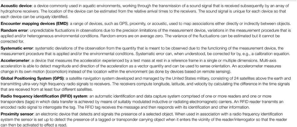
Table 1. Definitions.
We believe that the lack of error quantification in ABT studies is due to four factors. First, the study of device error will not directly lead to finding exciting biological phenomena: in fact, researching error comes at the cost of “real” discoveries in terms of time and resources. Moreover, studies at the interface of technology and biology could not be easily published due to the dearth of methodological journals. Secondly, progress in observation frequency and accuracy of ABT are so big relative to conventional methodologies (e.g., observations with binoculars) that device error is not the primary concern. Rather, sample size, automated processing, and correct analytical techniques for ecological interpretation were given a higher priority. Thirdly, computing power and statistical methods have only become available in the last decade. Finally, a framework to explore and quantify possible errors in ABT has been lacking.
While we believe that the first two causes for the limited attention are disappearing as new interdisciplinary and methodological journals have been founded (e.g., Journal of the Royal Society Interface or Methods in Ecology and Evolution), a general framework to discuss and analyze error is still lacking, though some previous studies focus specifically on error within a single device, such as GPS (Frair et al., 2010) or accelerometers (Shamoun-Baranes et al., 2012).
A New Framework for Error
Prima facie, each technology has a unique set of pathways by which error is introduced; we believe that these errors can be categorized by the processes that introduce the variation. We propose that there are three fundamental concepts that, when used to classify error, enable a comprehensive evaluation of error, regardless of technology: (1) the basic physical properties underlying data collection; (2) the conversion of raw data into useful variables; and (3) the subjectivity in the selected settings. We believe the use of this classification system will facilitate future work to recognize additional sources of error and, subsequently, to propose statistical methods to mitigate and/or quantify error. Here, we outline and discuss this classification scheme; we do not attempt to review the literature exhaustively, as we discuss numerous technologies to demonstrate the breadth of technologies that would benefit from this categorization.
Basic Physical Properties Underlying Data Collection
All ABT utilize physical properties to function: encounter mapping devices, RFID tags, and GPS devices all transmit and/or receive data through radio waves (varying from low to ultra-high frequencies), geo-locators detect fluctuations in light intensity, and accelerometers record changes in capacitance (see Table 1). While each technology measures a unique property or transmits data through a unique method, each physical property has generalizable characteristics, uncertainty in their measurement, and identifiable limitations.
For example, encounter mapping devices use radio waves to transmit unique animal IDs between tags (see Rutz et al., 2012). As radio waves spread in an environment, the energy contained within the radio wave decreases at a certain rate, and extrinsic factors, such as height above ground or the composition of the habitat, can alter this rate. Thus, a calibration to determine the rate at which radio waves degrade due to the behavior of the animal is essential.
Similarly, GPS devices transmit and receive ultra-high frequency radio wave signals from satellites. If any medium, like a vegetation canopy, is obstructing the travel path of the radio wave toward he sensor, it results in a lower fix rate and lower number satellites that can be detected—hence a lower location accuracy. Therefor also GPS devices require a calibration (as done in Jiang et al., 2008 and Williams et al., 2012; see Frair et al., 2010 for a more complete overview) to know the difference in performance under different types of vegetation so that, e.g., seemingly different intensities in habitat utilization by an organism can be interpreted correctly.
Radio waves degrade at a specified rate (different rates for different frequency of radio waves), and certain extrinsic factors can distort the signal, such as trees, the placement of the tag on the animal, and the ground (Rutz et al., 2015). Studies have quantified the degradation and variation of the signal due to external factors on signal strength and/or reliability. Devices utilizing radio waves, such as proximity devices, have significant variation in signal strength, suggesting that using these devices to differentiate distances may be problematic (Rutz et al., 2015).
Conversion of Raw Data into Useful Variables
When using ABT, the biological outcome is only as good as the conversion of raw data into useful variables. Three steps are generally taken during this conversion: (1) understanding the structure of the collected data, (2) determining the relationship between the raw data and the variable of interest, and (3) quantifying the error associated with the conversion. While many studies undertake steps 1 and 2, few studies have concentrated on quantifying error due to the conversion of raw data into useful variables.
Light based geo-location sensors, “geolocators”, combine a photoreceptor that converts incoming light levels into electrical energy with reference to an internal clock/calendar. To convert the light level and date-time information, use is made from a deterministic model (relating the time of local noon and midnight to the latitude, and day length to longitude). Usually the incoming light is limited to the 450 ±50 nm wavelength (a light-blue filter), because blue light predominates at the sun angles most appropriate for geo-location, just before sunrise and just after sunset (e.g., Lisovski et al., 2012).
On top of this well understood deterministic part of light based geo-location, there are large uncertainties involved due to factors like clouds, atmospheric refraction, atmospheric dust loading; foliage and feathers for terrestrial animals; depth and temperature effects for aquatic animals. Some of these factors can be corrected by measuring additional variables (such as pressure and temperature for aquatic; or cloudiness as observed at weather stations), whereas others have to be factored in as sources of noise. Several studies have been conducted to establish the uncertainty due to these factors, and also to provide a good protocol to calibrate sensors prior to deployment (Ekstrom, 2004; Fudickar et al., 2012; Bridge et al., 2013).
Subjectivity in the Settings Chosen
Nearly all ABT necessitate a priori selection of certain parameters. Generally, selecting parameters involves balancing the trade-offs between the highest resolution possible and the technological limits of the ABT, such as in the accessible memory and/or the capacity of the battery. Throughout the last decade, we have seen steady improvements in on-board memory and battery lifespans (Rutz and Hays, 2009), and may eventually see these limitations become non-existent.
One key parameter chosen is the frequency at which data is recorded. The rate of data collection determines the level of analysis data can be quantified, with higher rates of data collection allowing more a posteriori grouping of data for analysis, an indispensable step (at least for now) to examine data statistically. It is important to note, that we should maximize as much as possible the rate at which we collect data, as analytical methods allow for the comparison of higher-resolution data with older, less resolved data.
Another parameter commonly chosen is the power at which devices operate. In systems with passive RFID tags, for instance, the power of the receiver determines the distance (and rate) at which tags are being recognized. Since the detection range can, as a function of power, vary over an order of magnitude, it is crucial to know the exact power setting and its impact on this range in order to interpret the detection data (Nikitin and Rao, 2006; Finkenzeller, 2010). Hence the standardization of procedures in this context, or the availability of general calibration curves are required to compare results from different studies or interpret the results from a focal study at all (e.g., Pinter-Wollman et al., 2013).
A Four Step Workflow to Implement the Framework
The procedure we envision to implement the framework we outline in the previous section is based on 4 steps, which we labeled “Know”, “Identify”, “Evaluate”, and “Store”. Knowing consists of: (1) the physical principles of the technology, (2) the limitations of the technology, (3) the specific device and the context (i.e., the environment in which the device will be applied), and (4) experiences from others using the same device under comparable conditions. Knowing about the physics, sensor specification and context will enable a researcher to assess the likely influences in the specific location(s) the technology will be used, which is a required input to the next step: identify.
To “identify”, a model is constructed that describes the relationship between the variable of interest, relevant environmental factor(s), and the variable that is actually recorded and stored by the device. We call this model the observation model, since it is not a model for the biological system that we are studying, but only a way to translate the signal from the technology into the real-world variable that we are interested. Regardless, whether or not we have or need to build an existing observation model: experimental data or observational data with sufficient variability and data redundancy is required to evaluate model performance. In the ideal case, an appropriate observation model is already available and only needs to be evaluated (or calibrated and subsequently evaluated), and then the model can be used. If an observation model is not readily available, modeling from first principles (physical laws) or experimentation are the two remaining options. First, where possible, as much of the observation model should be defined on the basis of first principles (e.g., the effect temperature has on the functioning of a certain circuit, or the attenuation of a wave through a homogeneous medium at a given temperature). If the resulting model performs adequately, this could already form an endpoint. Otherwise, in addition, further parameterization with empirical relations may be required. For this task, experiments are required. In any case, an identified and calibrated observation model would need to be evaluated on a data set to which it was not calibrated.
Next, extra work is required to establish the robustness of the model in heterogeneous conditions. This is done in step 3, “Evaluate”, through a sensitivity and uncertainty analysis. For a sensitivity analysis, no real observations are required. Parameters or inputs are varied to evaluate how sensitive it is to perturbations. A sensitivity analysis is useful to find the parameters or inputs for which the observation model is particularly sensitive; these may subsequently be investigated in an uncertainty analysis. An uncertainty analysis applies realistic variability to a model to investigate how uncertainty propagates in the model and how it affects the results. If the resulting uncertainty is acceptable, the model is ready for use. In many situations it may turn out that the model will work within certain boundaries of input parameters. In these cases it is useful to specify the conditions in which the observation model performs or doesn't perform well. In addition, some questions require error estimation rather than quantification, requiring the evaluation of whether the error was estimated robustly.
Finally, we must properly store the observation model. With a simple parametric model one can store parameters, and parameter uncertainty. But with non-parametric models one should store the complete calibration dataset and algorithm; in that case, model uncertainty would need to be expressed in terms of predictive uncertainty. For any model, the assumptions underlying the model and the domain at which it is believed to be applicable. We strongly believe storing the model with uncertainty is essential to facilitate more transparency and use of the significant process just undertaken. Furthermore, the storage of raw data will aid error calculations in meta-analyses and facilitate more accurate evaluative criteria for inclusion.
An overview of both the framework and the workflow to implement is given in Figure 1.
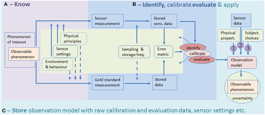
Figure 1. Illustration of the proposed framework as well the as four-step workflow to handle error in ABT. We start by defining a phenomenon of interest and the part of it that is observable (e.g., not a total population but only a small sample can be observed; only larger individuals can be tagged—note that this partial observation may lead to biases). The observable phenomenon can be measured by a sensor. When doing this, a number of factors influence the ultimate error of the observation model—these are contained in the central green box of the figure. The consequences from physical principles, sensor settings, environmental variability and animal behavior can often be known on the basis of deduction or previous studies (hence this part is contained in the purple zone (A), step 1 in the workflow). But when the effect of these factors on a sensor is not known, these should be part of experiments to identify this error. In addition to the aforementioned factors, the rate of sampling and actual storage of these observations as well as the choice of an error metric to quantify the adequacy of an observation are of great importance to identify, calibrate and evaluate an observation model (see the right part of the central green box). In the ideal situation, a “gold standard measurement” is used which is insensitive to the factors that impact the sensor of interest (as illustrated by the dashed arrows). By comparing the sensor of interest to a gold standard the development of an observation model goes through two main cycles: identification of the model structure and best possible parameter values (calibration is a final step in this) and evaluation of the derived model on independent data. Identification and Evaluation are steps two and three in the 4-step workflow and are highlighted in the blue area (B) of the figure. The processes of identification, calibration and evaluation typically require several experiments, hence the dotted arrows link back into the green box. After an observation model passes the evaluation, it can be applied to predict an observable phenomenon (with associated uncertainty) on the basis of sensor data. The final step in the workflow is then to store the result of the identification and evaluation experiments (C). The fact that this box encloses all the components of the figure emphasizes that this storage should include all relevant contextual information, modeling choices, sensor settings (etc.) along with the observation model, and should also link to application studies where this particular observation model has been used. The three encircled numbers in the model-application part at the right highlight the three main concepts to classify ABT error: (1) the basic physical properties underlying data collection; (2) the conversion of raw data into useful variables; and (3) the subjectivity in the selected settings. These concepts can only be adequately quantified if the entire workflow is rigorously applied.
Is There a Universal Protocol to Quantify Error?
No, but there are ways to think about error systematically, which help greatly to achieve error quantification. We propose a framework for this purpose. Each technology has its own unique limitations, necessitating different analytical or methodological approaches to mitigate error due to technological constraints. Yet, these confines exist in numerous technologies, and increasing the transparency through a common scheme will facilitate more rigorous studies and ensure the technological limitations refine and restrict the biological outcomes. Even in circumstances without opportunities to quantify different errors in ABT, the proper attribution of this error and the notion that it is irreducible will help to focus further developments (either in experimental work or development of new technologies).
Overall, organizing the process by which we think and calculate error is essential to ensure biological results are meaningful. To know, identify, evaluate and store, while recognizing the three processes introducing error into our data collections: physical properties, conversion from raw data into useful variables, and subjectivity in the settings. Specifically, recognizing similarities and differences between these devices will spur further integration of ideas from other devices to resolve the challenges of new devices, or old problems within a currently deployed device. Moreover, we believe the adoption of this scheme will facilitate feedback to designers, a necessary step to minimize certain types of error.
Conflict of Interest Statement
The authors declare that the research was conducted in the absence of any commercial or financial relationships that could be construed as a potential conflict of interest.
References
Böhm, M., Hutchings, M. R., and White, P. C. (2009). Contact networks in a wildlife-livestock host community: identifying high-risk individuals in the transmission of bovine TB among badgers and cattle. PLoS ONE 4:e5016. doi: 10.1371/journal.pone.0005016
Bridge, E. S., Kelly, J. F., Contina, A., Gabrielson, R. M., MacCurdy, R. B., and Winkler, D. W. (2013). Advances in tracking small migratory birds: a technical review of light-level geolocation. J. Field Ornithol. 84, 121–137. doi: 10.1111/jofo.12011
Brown, D. D., Kays, R., Wikelski, M., Wilson, R., and Klimley, A. P. (2013). Observing the unwatchable through acceleration logging of animal behavior. Anim. Biotelem. 1, 20. doi: 10.1186/2050-3385-1-20
Butler, P. J., Woakes, A. J., and Bishop, C. M. (1998). Behaviour and physiology of Svalbard Barnacle Geese Branta leucopsis during their autumn migration. J. Biol. 29, 536–545. doi: 10.2307/3677173
Ehrenberg, J. E., and Steig, T. W. (2002). A method for estimating the “position accuracy” of acoustic fish tags. ICES J. Mar. Sci. 59, 140–149. doi: 10.1006/jmsc.2001.1138
Ekstrom, P. A. (2004). An advance in geolocation by light. Mem. Natl. Inst. Polar Res., Spec. Issue 58, 210–226.
Finkenzeller, K. (2010). RFID Handbook: Fundamentals and Applications in Contactless Smart Cards, Radio Frequency Identification and Near-Field Communication, 3rd Edn. New York, NY: Wiley.
Frair, J. L., Fieberg, J., Hebblewhite, M., Cagnacci, F., DeCesare, N. J., and Pedrotti, L. (2010). Resolving issues of imprecise and habitat-biased locations in ecological analyses using GPS telemetry data. Philos. Trans. R. Soc. B Biol. Sci. 365, 2187–2200. doi: 10.1098/rstb.2010.0084
Fritts, S. H., Bangs, E. E., Fontaine, J. A., Johnson, M. R., Phillips, M. K., Koch, E. D., et al. (1997). Planning and implementing a reintroduction of wolves to Yellowstone National Park and central Idaho. Restoration Ecol. 5, 7–27. doi: 10.1046/j.1526-100X.1997.09702.x
Fudickar, A. M., Wikelski, M., and Partecke, J. (2012). Tracking migratory songbirds: accuracy of light−level loggers (geolocators) in forest habitats. Methods Ecol. Evol. 3, 47–52. doi: 10.1111/j.2041-210X.2011.00136.x
Hays, G. C., Forman, D. W., Harrington, L. A., Harrington, A. L., MacDonald, D. W., and Righton, D. (2007). Recording the free−living behaviour of small−bodied, shallow−diving animals with data loggers. J. Anim. Ecol. 76, 183–190. doi: 10.1111/j.1365-2656.2006.01181.x
Hull, C. L. (1997). The effect of carrying devices on breeding royal penguins. Condor 99, 530–534. doi: 10.2307/1369962
Jiang, Z., Sugita, M., Kitahara, M., Takatsuki, S., Goto, T., and Yoshida, Y. (2008). Effects of habitat feature, antenna position, movement, and fix interval on GPS radio collar performance in Mount Fuji, central Japan. Ecol. Res. 23, 581–588. doi: 10.1007/s11284-007-0412-x
Krause, J., Krause, S., Arlinghaus, R., Psorakis, I., Roberts, S., and Rutz, C. (2013). Reality mining of animal social systems. Trends Ecol. Evol. 28, 541–551. doi: 10.1016/j.tree.2013.06.002
Lisovski, S., Hewson, C. M., Klaassen, R. H., Korner−Nievergelt, F., Kristensen, M. W., and Hahn, S. (2012). Geolocation by light: accuracy and precision affected by environmental factors. Methods Ecol. Evol. 3, 603–612. doi: 10.1111/j.2041-210X.2012.00185.x
Nikitin, P. V., and Rao, K. S. (2006). Theory and measurement of backscattering from RFID tags. Antennas Propagation Mag. IEEE 48, 212–218. doi: 10.1109/MAP.2006.323323
Okuyama, J., Kataoka, K., Kobayashi, M., Abe, O., Yoseda, K., and Arai, N. (2012). The regularity of dive performance in sea turtles: a new perspective from precise activity data. Anim. Behav. 84, 349–359. doi: 10.1016/j.anbehav.2012.04.033
Patterson, T. A., McConnell, B. J., Fedak, M. A., Bravington, M. V., and Hindell, M. A. (2010). Using GPS data to evaluate the accuracy of state-space methods for correction of Argos satellite telemetry error. Ecology 91, 273–285. doi: 10.1890/08-1480.1
Pinter-Wollman, N., Hobson, E. A., Smith, J. E., Edelman, A. J., Shizuka, D., de Silva, S., et al. (2013). The dynamics of animal social networks: analytical, conceptual, and theoretical advances. Behav. Ecol. 25, 242–255. doi: 10.1093/beheco/art047
Rutz, C., Burns, Z. T., James, R., Ismar, S. M., Burt, J., Otis, B., et al. (2012). Automated mapping of social networks in wild birds. Curr. Biol. 22, R669–R671. doi: 10.1016/j.cub.2012.06.037
Rutz, C., and Hays, G. C. (2009). New frontiers in biologging science. Biol. Lett. 5, 289–292. doi: 10.1098/rsbl.2009.0089
Rutz, C., Morrissey, M. B., Burns, Z. T., Burt, J., Otis, B., St Clair, J. J., et al. (2015). Calibrating animal-borne proximity loggers. Methods Ecol. Evol. doi: 10.1111/2041-210X.12370
Shamoun-Baranes, J., Bom, R., van Loon, E. E., Ens, B. J., Oosterbeek, K., and Bouten, W. (2012). From sensor data to animal behaviour: an oystercatcher example. PLoS ONE 7:e37997. doi: 10.1371/journal.pone.0037997
Shillinger, G. L., Bailey, H., Bograd, S. J., Hazen, E. L., Hamann, M., Gaspar, P., et al. (2012). Tagging through the stages: technical and ecological challenges in observing life histories through biologging. Mar. Ecol. Prog. Ser. 457, 165–170. doi: 10.3354/meps09816
Williams, D. M., Quinn, A. D., and Porter, W. F. (2012). Impact of habitat-specific GPS positional error on detection of movement scales by first-passage time analysis. PLoS ONE 7:e48439. doi: 10.1371/journal.pone.0048439
Keywords: animal-borne device, bio-logging, calibration, error, observation model
Citation: Burns ZT and van Loon EE (2015) A framework to classify error in animal-borne technologies. Front. Ecol. Evol. 3:55. doi: 10.3389/fevo.2015.00055
Received: 19 January 2015; Accepted: 10 May 2015;
Published: 27 May 2015.
Edited by:
Peng Liu, Chinese Academy of Sciences, ChinaReviewed by:
Clive Reginald McMahon, University of Tasmania, AustraliaMaja Borry Zorjan, Université de Versailles Saint-Quentin-en-Yvelines, France
Karen Evans, Commonwealth Scientific and Industrial Research Organisation, Australia
Copyright © 2015 Burns and van Loon. This is an open-access article distributed under the terms of the Creative Commons Attribution License (CC BY). The use, distribution or reproduction in other forums is permitted, provided the original author(s) or licensor are credited and that the original publication in this journal is cited, in accordance with accepted academic practice. No use, distribution or reproduction is permitted which does not comply with these terms.
*Correspondence: E. Emiel van Loon, Computational Geo-Ecology, Institute for Biodiversity and Ecosystem Dynamics, University of Amsterdam, Science Park 904, Amsterdam 1098 XH, Netherlands, e.e.vanloon@uva.nl