 Marcos Vinícius Gualberto Barbosa da Silva1,2 Curtis P. Van Tassell2* Tad S. Sonstegard2 Jaime Araujo Cobuci3 Louis C. Gasbarre2
- 1 Bioinformatics and Animal Genomics Laboratory, Embrapa Dairy Cattle, Juiz de Fora, Minas Gerais, Brazil
- 2 Bovine Functional Genomics Laboratory, Agricultural Research Service, United States Department of Agriculture, Beltsville, MD, USA
- 3 Animal Science Department, Federal University of Rio Grande do Sul, Porto Alegre, Rio Grande do Sul, Brazil
Accurate genetic evaluation of livestock is based on appropriate modeling of phenotypic measurements. In ruminants, fecal egg count (FEC) is commonly used to measure resistance to nematodes. FEC values are not normally distributed and logarithmic transformations have been used in an effort to achieve normality before analysis. However, the transformed data are often still not normally distributed, especially when data are extremely skewed. A series of repeated FEC measurements may provide information about the population dynamics of a group or individual. A total of 6375 FEC measures were obtained for 410 animals between 1992 and 2003 from the Beltsville Agricultural Research Center Angus herd. Original data were transformed using an extension of the Box–Cox transformation to approach normality and to estimate (co)variance components. We also proposed using random regression models (RRM) for genetic and non-genetic studies of FEC. Phenotypes were analyzed using RRM and restricted maximum likelihood. Within the different orders of Legendre polynomials used, those with more parameters (order 4) adjusted FEC data best. Results indicated that the transformation of FEC data utilizing the Box–Cox transformation family was effective in reducing the skewness and kurtosis, and dramatically increased estimates of heritability, and measurements of FEC obtained in the period between 12 and 26 weeks in a 26-week experimental challenge period are genetically correlated.
Introduction
Gastrointestinal nematode infection causes significant losses to livestock industries worldwide. It reduces meat and milk production, increases mortality, requires anthelmintic use, and often results in changes in herd management. In most cattle-producing areas of the world, infection by helminth parasites (particularly gastrointestinal nematodes) is a cause of substantial production losses (Barger, 1993). In New Zealand anthelminthic expenses are about $27.9 million/year (Bisset, 1994), and in the U.S.A. these parasites cost to the American livestock industry, approximately, $2 billion/year in lost productivity and increased operating expenses (Sonstegard and Gasbarre, 2001). These authors also noted that anthelmintics are frequently used to prevent potential economic losses, resulting in an increased anthelmintic resistance in cattle and increased consumer concern about drug residues in animal products.
Selecting animals with enhanced resistance to parasites can reduce pasture contamination, decrease the dependence on anthelmintics, and reduce selection for drug resistance. A genetic component to host resistance in cattle has been reported by Gasbarre et al. (1990), where heritability of parasite resistance was estimated to be approximately 0.30, allowing for moderate genetic progress. Gasbarre et al. (2002) believe that QTL mapping and marker-assisted selection (MAS) could be used to accelerate genetic improvement.
Fecal egg count (FEC) is used to identify and quantify gastrointestinal parasite infestations. FEC values are not normally distributed, and a small percentage of the herd is responsible for the majority of parasite transmission (Gasbarre et al., 1990). This overdispersion of FEC values was first described by Crofton (1971a,b) and has been reported in other cattle populations. In this overdispersed distribution, the value of the SEM frequently exceeds the value of the mean, and as such most individuals have relatively low fecal FEC values, and a small percentage of animals, estimated to be between 15 and 25% of the total population (Anderson and May, 1985), exhibit high FEC values. This pattern strongly suggests genetic management of a small percentage of the herd could considerably reduce overall parasite transmission.
In order to produce distribution of FEC that is close to normality, logarithmic transformations of the data have been used before analysis (Nødtvedt et al., 2002). The most common transformations are y = ln(FEC + 1) (Torgerson et al., 2005) and y = ln(FEC + 100) (Morris et al., 2003), where ln is the natural (base e) logarithm. Nevertheless, normalization of the distribution is not achieved in most cases, especially when data are extremely skewed (Wilson and Grenfell, 1997). In addition, type I errors are likely to be common and type II errors are increased when using a log-transformed method (Wilson et al., 1996).
Accurate genetic evaluation of livestock is based on appropriate modeling of phenotypic measurements. Phenotypes measured several times over the life of the animal are called longitudinal data. Production of milk, fat, and protein in dairy cattle and growth in beef cattle are examples of this type of data. The ability of RRM to model a separate lactation or growth curves for each animal and to account for differences in shapes of permanent and temporary environmental effects curves has made these models extremely useful for dairy cattle evaluations (Strabel and Jamrozik, 2002).
As noted above, also used in other species, FEC is commonly used to measure resistance or susceptibility to nematodes. A series of repeated FEC measurements may provide information about the population dynamics of a group or individual. An infection curve can be calculated for each animal using weekly measurements. These measures have been used to separate calves into the following categories: Type I – resistant animals that are innately immune and never demonstrated high FEC values, Type II – animals that have acquired immunity over time, and Type III – immunologically non-responsive animals that are susceptible to infestation.
Advantages of RRM for FEC analysis include: (a) removal of environmental variation in phenotypic data by considering the specific common environmental effects of each record; (b) use of a larger number of records per animal, rather than a single number such as mean, peak, or maximum value, (c) more accurate estimation of genetic and permanent environmental effects influencing FEC and (d) more accurate assignment of animals into resistant, acquired, or susceptible phenotypes.
The objectives of the present study were to use an extension of the Box–Cox transformation to approach normality and to determine the efficiency of the transformation and random regression models (RRM) for analyzing FEC data.
Materials and Methods
Resource Population
A divergent selection program for parasite resistance was initiated at the Beltsville Agricultural Research Center using parental stock that originated from the Wye Angus herd at the University of Maryland. Once initial breeding females were identified, semen from high and low FEC bulls was used to produce calves of the desired phenotypes.
Calves were kept with their dams on pastures with extremely low numbers of parasites prior to weaning. When the median age of the contemporary group was 205 days, calves were weaned and placed on pastures infected with the two most common nematode parasites of US cattle, Ostertagia ostertagi and Cooperia oncophora. Calves were monitored weekly for the following: FEC, serum pepsinogen level, serum antibodies of the IgG1, IgG2, IgA, and IgM subclasses to Ostertagia and Cooperia crude antigens, blood eosinophil levels, complete blood count (CBC; hematocrit, hemoglobin, red blood cell count, white blood cell count, mean cell volume), body weight, hip height, and scrotal circumference of the bull calves. The calves were kept on pasture for a minimum of 120 days, and animals were selected as replacement breeders for re-challenge experiments, or for immediate post-mortem collection of parasitological and immunological data. Data collected post-mortem included: parasite species and numbers recovered, sex, and length of worms, enumeration of Ostertagia- and Cooperia-specific T cells in the abomasal and mesenteric lymph nodes by limiting dilution analysis, weight of abomasal lymph nodes, enumeration by flow cytometry of CD3, CD4, CD8, IL2-receptor, B-cell marker, surface IgM, and T-cell receptor positive cells in the abomasal and mesenteric lymph nodes, and semi-quantitative competitive PCR measure of mRNA expression of IL2, IL4, IL10, IL13, IL15, IL18, IFN, TNF, and TGF in abomasal and mesenteric lymph nodes (Gasbarre et al., 2002).
To date, 410 progeny have been tested in this parasite challenge system. Complete pedigree records for this population tracing back to the original founding animals of the Wye herd have been assembled. Initial pedigree analysis of the resource population reveals that >90% of the animals are paternally descended from a Wye bull born in 1944. This extreme relationship to a single bull may have resulted from selection for a single major histocompability complex (MHC) haplotype. DNA for genetic analysis has been acquired from all animals from the resource population and over 70 sites in the historic pedigree (Gasbarre et al., 2002).
Data Transformation
In order to obtain the skewness and kurtosis, as well as in the analyzes by REML, the response variable yi (mean or largest value of FEC) was analyzed using ln(count + 100) or on a  scale obtained from the Box–Cox transformation family, in which
  or
or  An adaptation of the algorithm proposed by Hyde (1999 was used to estimate the maximum likelihood estimate of λ. In the random regression analyzes, different values of λ were used (1, 0.5, 0.14, 0, −0.5, and −1) to compare transformation efficiency, denoted, MA, ML, ZE, M5, and M1, respectively.
Estimation of Variances and Covariances by REML
Between 1992 and 2003, 6375 observations of FEC were collected from 410 animals from the BARC Angus herd. Only FEC data collected 4–26 weeks after an animal entered the experiment were considered in the analyses.
Contemporary groups were defined as groups of animals entering an experiment together. There were 17 contemporary groups in the study. Estimation of the genetic parameters in this analysis involved partitioning phenotypic (co)variances between relatives into its components using the degree of relationship between animals. A linear mixed model for one trait and one record per animal can be written as:

where y is a vector of observations for FEC (mean or highest value, untransformed or transformed by log or Box–Cox); X is the known incidence matrix relating observations to fixed effects; β is a vector of fixed effects (contemporary groups, sex of the animal, and age at test); Zu is a known incidence matrix relating observations to random animal effects; u is the vector of animal additive genetic random effects,  ; and e is the vector of residual effects,
A repeated measure, mixed model analysis was used to estimate permanent environmental variances:

where y is the vector of observations for monthly FEC (untransformed or transformed by log or Box–Cox); β, u, and e are as defined in (1), and  is a vector of random permanent environmental effects with incidence matrix Zc.
From the variance components, two parameters were defined: heritability,  , and the fraction of permanent environmental variance,
  In addition, repeatability (r) was defined as the sum of h2 and c2.
Heritabilities were estimated using the animal model with the Multiple Trait Derivative Free Restricted Maximum Likelihood (MTDFREML) software program of Boldman et al. (1995). The numerator relationship matrix, A, was constructed using complete pedigree information among all animal in the study and relevant ancestors using the algorithm described by Quaas (1976).
Heritabilities were estimated using single-trait analyses. Starting values of the genetic and environmental variances for single-trait analyses were estimated using results from the MIXED procedure in SAS (1996). Single-trait analyses were run using low (10−4) and high (10−9) convergence criteria.
Estimated breeding values (EBV) for FEC records before and after transformations (ln and Box–Cox) were compared. Correlations between the three sets of EBV and percentage of animals selected with all three evaluations, under difference selection intensities (100, 50, 25, 10, 5, and 1%), were calculated.
Estimation of Variances and Covariances by Random Regression Model
The following RRM was utilized to estimate genetic parameters for FEC:
where yijkl is FEC observation of animal l during week k, within classes i (year) and j (sex–age), YEi is the fixed effect of year of collection (i = 1, 2,…, 12). SAj is the fixed effect of classes sex–age (j = 1, 2, …14). βm, is the vector of regression coefficients fixed specifically to describe the average population curve; akm and pkm vectors of random regression coefficients which respectively describe additive genetic and permanent environment effects, and eijkl, random residual effect associated with yijkl; Zklm, represents the mth parameter of Legendre polynomials of order 2, 3, or 4. Residual variance was considered constant over the collection period (week). Legendre polynomials were standardized by to range from −1 and 1 as proposed by Kirkpatrick et al. (1990).
Estimation of the (co)variance components by the RRMs produced a matrix containing (co)variances of random regression coefficients. The variances in FEC during different weeks are obtained from the (co)variance matrix and the vector that contains (co)variables which individually describe the shape of the FEC curve of the animals.
The estimates of genetic variance  and permanent environmental variance
  determined by RRM, in FEC during week k were calculated as:

and

where Ĝ and  are matrices of genetic and permanent environmental variances and covariances between random regression coefficients, respectively; zk = (co)variables related to a specific FEC measured during week k.
The estimation of genetic and permanent environmental (co)variances between two FEC during week k,  and
and  for k′ ≠ k, were obtained by:
and
where Ĝ and zk are as described above, and  transpose of zk, for k′ ≠ k.
Variance and (Co)variance matrices of the regression coefficients (additive genetic – Ĝ and permanent environment – ) too necessary for calculation of heritability, repeatability and genetic correlations were computed using REMLF90 package (Misztal, 2005). Convergence was declared when the change in −2log likelihood (L) between rounds was 10−9.
Estimation of Genetic Parameters by Random Regression Model
The estimation of heritability for FEC during week k, using RRM were obtained by:
The estimation of repeatability for FEC during week k were obtained by:
The estimation of genetic correlations between FEC k′ and FEC k were calculated by:
where k′ and k = FEC information,  = estimate of residual variance, and
  are as described previously.
Comparison of the Models in Random Regression Analysis
Selection of models was based on Akaike’s information criterion (AIC; Akaike, 1973). Akaike (1973) proposed a simple and useful criterion for selecting the best-fit model among alternative models: AIC = −2logL + 2. p Differences among AIC values are important, not the absolute size of AIC values. The model with the lowest AIC is considered the best. Some experiences verify the applicability of AIC in model selection (Burnham and Anderson, 1998). Another widely used information criterion is the Bayesian–Schwarz information criterion (BIC), which takes into account model uncertainty as well. The Bayesian–Schwarz information criterion is stricter than the AIC, and is defined as BIC −2logL + p.ln(n − r) where p refers to the number of model parameters, where n is equal to the number of records used in the analysis and r is the rank of the matrix X, which is the incidence matrix for fixed effects (Burnham and Anderson, 1998). Both tests permit comparisons between non-nested models and penalize models with more parameters, but the BIC favors more parsimonious models. Lower values to AIC and BIC indicate best adjusting.
Results
Optimum Box–Cox Transformation
Descriptive statistics of FEC for each week and overall data are presented in Table 1 and Figure 1. Weekly data were distributed uniformly from the 4th to 17th week. Estimates of variability within-weeks were large. Variability was associated with the mean; SD tended to be larger and coefficients of variation smaller as the mean decreased. The overall mean, SD, and coefficient of variation were 61.86 ± 83.79 and 135.46%.
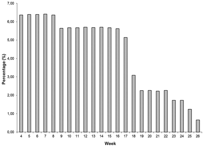
Figure 1. Distribution of fecal egg count (FEC) samples (n = 6375).
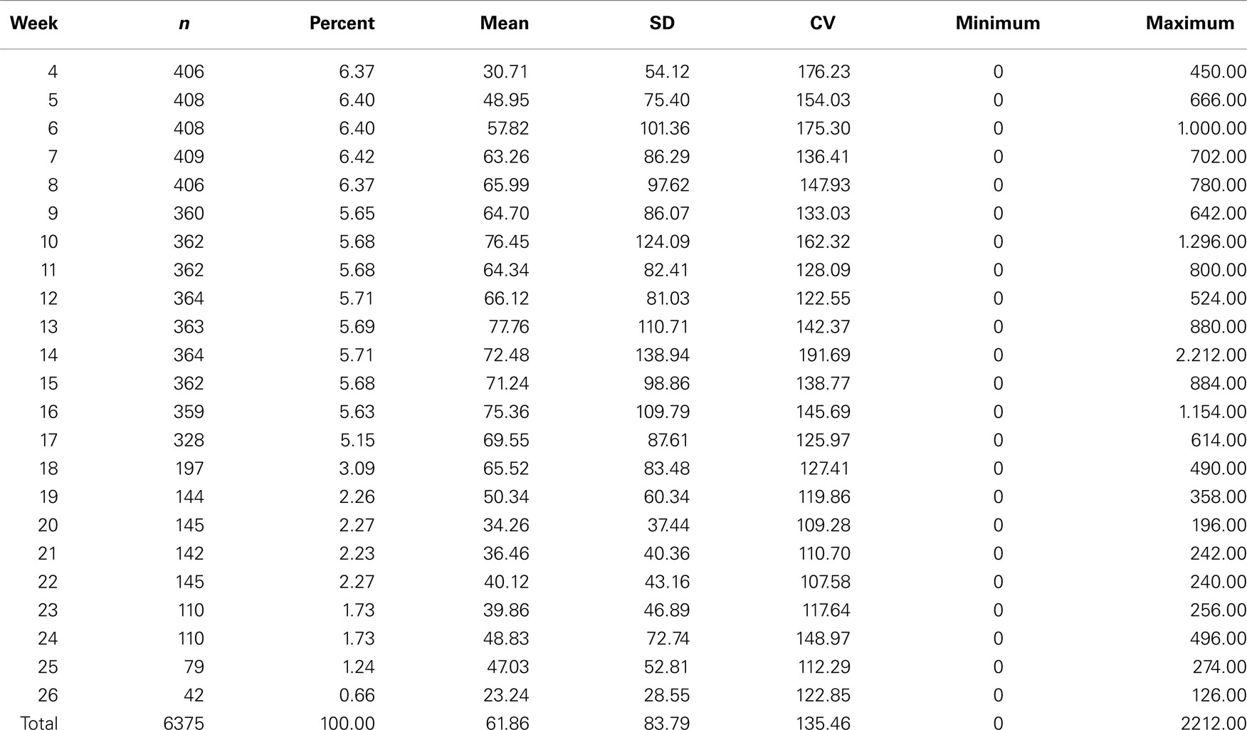
Table 1. Descriptive statistics for fecal egg count (FEC) for weeks and overall data for Angus cattle.
Skewness and kurtosis coefficients for the variables analyzed are presented in Table 2. Positive skewness and kurtosis are typical in FEC data. Values for non-transformed FEC values and those transformed using the Box–Cox (BC) are shown for all three functions of FEC. Estimates of λ obtained by ML were: 0.139 (mean value), 0.149 (largest value), and 0.132 (all values), indicating that the logarithmic transformation typically used for FEC data is not optimal, as λ was greater than 0 for all variables.
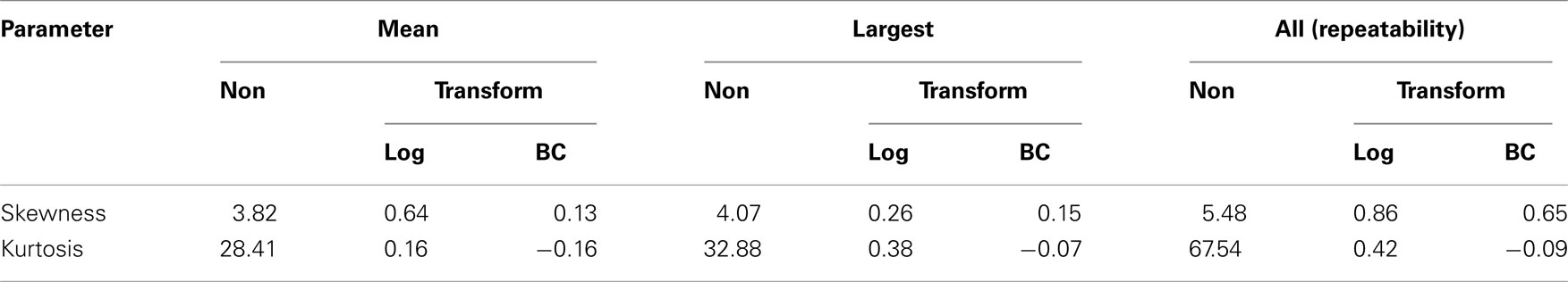
Table 2. Values of skewness and kurtosis for non-transformed (Non), log, and Box–Cox (BC) transformed data.
The effectiveness of FEC transformation using  is illustrated in Table 2. Transformation reduced coefficients of asymmetry in all the variables studied, thereby improving the distribution of FEC. Although expected values for skewness and kurtosis for a normal distribution are zero, in a general way, the values from data after Box–Cox transformation were closer to zero than those for non-transformed and log-transformed.
(Co)variance Components and Genetic Parameters Estimated by REML for FEC
Summaries of the (co)variance components and genetic parameters estimated by different models and methodologies are shown in Tables 3 and 4. The heritabilities for FEC (mean and largest values) using data transformed by Box–Cox were greater than those estimates obtained for non-transformed or ln transformation using the same model. Comparing all the results, it seems that when the normality distribution was not met, the conventional method of estimation failed. Increases in the heritability after use of Box–Cox transformation were related by Besbes et al. (1993) and Ünver et al. (2004), in egg production.
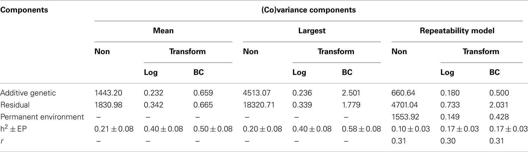
Table 3. Additive genetic, residual (co)variance and heritabilities estimates, obtained using non-transformed (Non) and log and Box–Cox (BC) transformed data for Angus cattle.
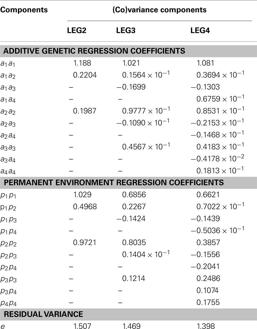
Table 4. Additive genetic, permanent environment and residual (co)variance estimates of the regression coefficients, obtained using different random regression models.
Effect of the Box–Cox Transformation on Selection Decisions
Spearman correlation coefficients between EBV of candidates for selection were estimated using non-transformed and ln- and Box–Cox transformed data. In all intensities of selection (100, 50, 25, 10, 5, and 1%) the correlations between non-transformed data and ln or Box–Cox transformations were lower than the correlations between ln and Box–Cox, decreasing linearly from 91% (non-transformed and Box–Cox) and 86% (non-transformed and ln), when intensity of selection was 100%, to 0%, when 1% of the population was selected.
The correlations between ln and Box–Cox transformation had a similar tendency. The correlations in all intensities of selection (100, 50, 25, 10, 5, and 1%) were 0.97, 0.91, 0.88, 0.64, 0.63, and 1.0, respectively. Despite this last correlation being equal 1.0, only two animals were present in both ranks (ln and Box–Cox). In all other situations, the ranks between both transformations disagree as well; in other words, some animals were present in a rank by ln and were not present in a rank by Box–Cox. The percentage of disagreement were equal to 10, 10, 15, 25, and 60%, when the intensities of selection were 50, 25, 10, 5, and 1%, respectively.
The percentage of animals which would be selected in these three evaluations follows a different trend. Also that the higher the selection intensity, the lower these percentage are. Consequently, non-normality has a major effect on the selection decisions when a small proportion of animals have to be selected.
(Co)variance Components and Genetic Parameters Estimated by Random Regression Models for FEC
The summary of the analysis in relation to the log of likelihood function to random regression analysis is presented in the Table 5. Akaike (AIC) and Bayesian (BIC) information criteria for polynomial models of orders 2, 3, and 4 were as follows: 10109, 10051, and 9961; 10157, 10138, and 10103. The quality of the adjustments generally improved with the number of parameters in the model (Table 5). Based on these values, a polynomial model of order 4 was used.
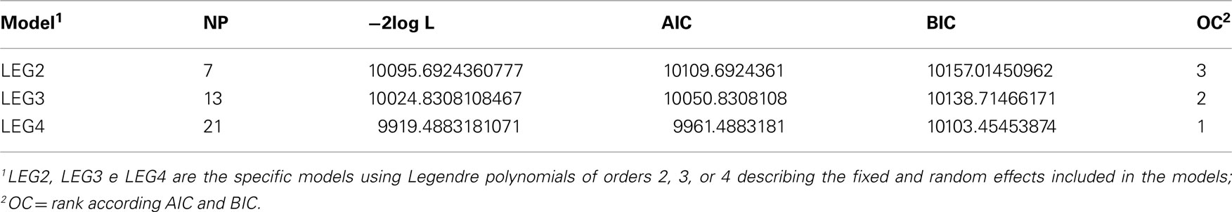
Table 5. Number of parameters (NP), −2log value of the likelihood function (−2log L), Akaike (AIC), and Bayesian information criterion (BIC), according differents random regression models.
In total, 7, 13, and 21 (co)variance components were simultaneously estimated by model LEG2, LEG3, and LEG4, respectively. Estimates of residual variance decreased as the order of Legendre polynomial in model increased and were as 1.507, 1.469, and 1.398.
Estimates of the additive genetic variance of FEC for different values of λ across the time using model LEG4 is shown in Figure 2. In general, the transformations M1, M5, ZE, and MA showed similar tendencies and low values during the entire evaluation period, with opposite tendencies in ML transformation or in the non-transformed data. These last two datasets showed crescent values in relation to additive genetic variance until week 12; so, they decreased significantly from that until week 24 before increasing again. The increase during the final period may have occurred because of the reduced number of available FEC data points (Table 1). This tendency has been observed in studies involving RRMs and different traits, i.e., milk production (Kachman, 2004). Permanent environmental variance obtained for the different transformations follow a similar trend to the additive genetic variance (Figure 3), however, with larger magnitudes. Estimates of the residual variance of FEC for different values of λ across the time are shown in Figure 4. As a consequence of the transformation, the scale of measurement has changed. Thus, the additive genetic, permanent environment and residual variances on the transformed and the non-transformed data are not comparable.
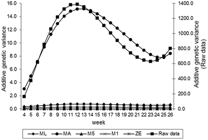
Figure 2. Estimates of additive genetic variance of fecal egg count (FEC) over time for different values of λ.
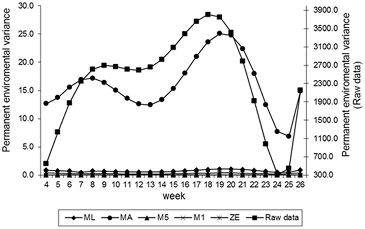
Figure 3. Estimates of permanent environment variance of fecal egg count (FEC) over time for different values of λ.
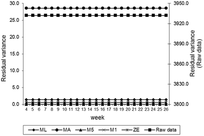
Figure 4. Estimates of residual variance of fecal egg count (FEC) over time for different values of λ.
Figure 5 presents estimates of FEC heritability for different values of λ across the time that data were collected. Estimates of h2 vary with values of λ used in transforming FEC. Greater values of heritability for weekly counts were found for values of λ equal to 0.14 (obtained by ML), 0 (log transformation), and 0.5, indicating that FEC is a trait with moderate heritability and possible to select for. When the estimates of λ obtained by ML and log were used, the value of h2 for whole period (weeks 4–26, considering as one trait) was 0.58 for both of them. This result was expected because analyzing all records by an animal using RRMs, the distribution is nearly normal. These estimates were greater than those typically estimated (0.3–0.4) from traditional evaluation of the trait (Sonstegard and Gasbarre, 2001) and similar to estimates obtained using mean and largest values transformed data by Box–Cox in this study. Comparison between results should be made with caution because of differences in models and methods used to estimate variance components as well as the data transformation. In a comparison of estimates of breeding values based on non-transformed and Box–Cox transformed data, Savas et al. (1998) found Box–Cox transformed data was more accurate. The shape of the heritability curve with lower values at the beginning of the experiment was predictable, as response to the challenge was highly variable.
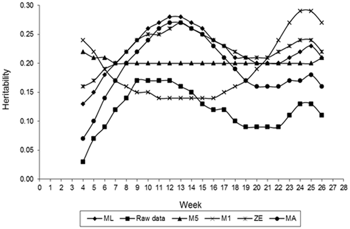
Figure 5. Estimates of heritability of fecal egg count (FEC) over time for different values of λ.
Estimates of FEC repeatability for different values of λ across the time shown in Figure 6. Similar to the heritability, estimates of the repeatability also varied with values of λ used in transforming FEC. Smaller values of repeatability for weekly counts were found for values of λ equal to −0.5 (M5) and −1. (M1). The exception to this observation was the initial and final period of collection FEC recording. Values maintained constant up to the 12th week and then came high. In general, these values indicated that FEC is a trait with high repeatability, which is an important characteristic for implementation into an animal breeding program. Selection is likely more efficient when it is based on records between weeks 7 and 22. When the estimate of λ obtained by ML was used, the value of repeatability for whole period (weeks 4–26, when considered as one trait) was 0.93. A similar result was obtained using ln transformation. Using ln-transformed data, or cube root-transformed data, may increase the repeatability estimate relative to using non-transformed values (Morris et al., 2004). These estimates are higher than the results from Morris et al. (2004). Those authors, using least squares, obtained a repeatability estimate for FEC in dairy calves equal to 0.45, was somewhat higher than that found in grazing beef calves (0.21) in an previous study (Morris et al., 2002).
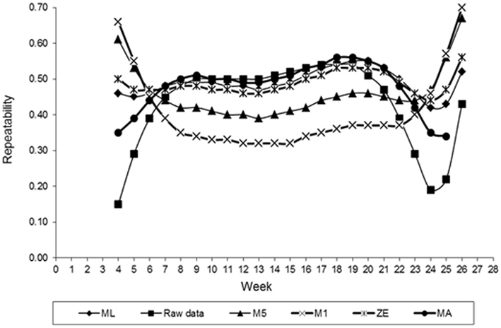
Figure 6. Estimates of repeatability of fecal egg count (FEC) over time for different values of λ.
Figure 7 represents the estimates of genetic correlations among all FEC measurements in the whole period (weeks 4–26). This was obtained using the RRM and adjusting by the fourth order Legendre polynomial to the different transformations in the FEC (λ values). It can be observed that the magnitudes of the correlations follow similar tendencies, when λ values equal to 0.14 (ML), zero (ZE), or one (MA) were used. When all the correlations generated by FEC transformed using λ values equal to 0.5 (M5) and −1 (M1) were compared together, the behavior was analogous. However, larger genetic correlations (>0.9) were obtained using non-transformed data (raw data). In general, genetic correlations obtained using data transformed by ML, ZE, and MA suggested that the FEC between 12th and 26th are correlated through the genetic component (0.80–1.00).
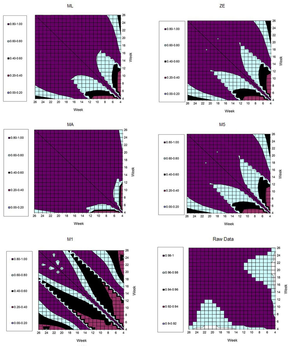
Figure 7. Estimates of genetic correlation among fecal egg count (FEC) weekly measures, according different kinds of transformations (λ values).
The curves of the EBV, predicted by the LEG4 model for 5 different animals, during the whole period analyzed are illustrated in Figure 8. These EBV curves indicate that there are genetic differences among animals in relation to parasite resistance. These results that show the EBV mean curve to the 410 animals of the population. It can be observed that from week 12, the mean of the EBV decreased constantly to week 22, probably because the animals with acquired immunity and immune are the most at this population. Therefore, they can be influencing the mean by an overrepresentation of low values. The curve ascends from weeks 22 to 26, and is probably an artifact caused by a lack of information about FEC in these last 3 weeks.
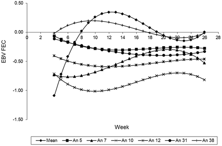
Figure 8. Estimates breeding values of FEC (EBVFEC) over time for different animals (λ = ML).
In the Figure 9, animals 144 and 185 showed curves with low and constant values during the whole period. These can classify them as immune. By the other hand, the animals 75 and 132 showed curves with higher values in the beginning of the experiment, but their values were reducing over time. So, these animals can be classified as Type III or acquired immunity. Finally, animals 25 and 112 can be characterized as susceptible, because their FEC values increased over time, especially the animal 112, in which all the measurements are bigger than the mean value in all weeks.
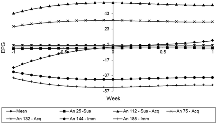
Figure 9. Estimates of the resistance using the random regression curves over time for different animals.
Discussion
Box–Cox Transformation
The assumption of normality is very important from the statistical point of view, but there is not much information about non-normality of data and its effect on the (co)variance components and genetic parameters. In the variance component analysis there is evidence that lack of normality influenced the estimates as described by Brownie et al. (1990). Small values of kurtosis and asymmetry in the analysis of variance also are important indicators about how the normality deviation can influence the estimates (Scheffé, 1959). The lack of normality can also influence negatively the estimates of fixed effects and heterogeneity of error variance (Cochran and Cox, 1978). Savas et al. (1998) noted that lack of normality is a possible source of error when (co)variance components and genetic parameters are estimated, while Ibe and Hill (1988) affirmed that non-linearity and heterogeneity may lead to biased estimates of parameters and reduce the efficiency of selection index and best linear unbiased prediction (BLUP).
Box–Cox transformation of FEC data should also enhance QTL mapping sensitivity and accuracy, based on the observation by Ibe and Hill (1988) that non-linearity and heterogeneity may lead to biased estimates of parameters and reduce the efficiency of selection index and BLUP. According to Tilquin et al. (2001), most QTL mapping methods assume that phenotypes are normally distributed, and this assumption is clearly violated for many measures of disease resistance. Therefore, improving normality should improve behavior of the statistical tests. In targeting the normality of the random effects of the model, the Box–Cox transformation should provide improved estimates of the random effects (Gurka et al., 2006). Mostly importantly, since previous research has indicated that accurate estimation and inference on the random effects is dependent on the assumption of normality (Verbeke and Molenberghs, 2000).
The Box–Cox transformation produced data which followed a normal distribution more closely than the original and ln transformation (Table 2). While this transformation does not guarantee that the transformed data are normal, it does reduce problems with estimation, prediction, and inference (Hyde, 1999). Since the proposed model is based on the Box–Cox family of power transformations, the advantage of this approach is its applicability to a larger class of problems where normality of distributions, constancy of error variance and/or simplicity of the model structure are required. In the variance component analysis there was evidence that lack of normality influenced the estimates as described by Brownie et al. (1990). Transformation of this type of data may result in more precise estimates of fixed effects in analyses of variance, as well as reduced proportion of residual variance and larger fraction of the total variance attributed to random effects.
Genetic Parameters Estimated by REML for FEC
The results of this study indicate that the use of a power transformation of the response variable in components of variance model improves the quality of prediction of FEC genetic parameter estimates. The proposed model provides a reasonable (if not perfect) fit to the data considered in this study. Therefore one should be comfortable to use the Box–Cox power transformations in FEC analysis.
When more than one record per animal was analyzed by a repeatability model, both ln and Box–Cox transformations provided similar results. Banks et al. (1985) reported that REML is robust, in terms of expectation, to skewed distribution in estimating variance components. Results obtained in this study show that this robustness is verified only for slight skewness, as is the case for FEC using all records by animal. However, it is interesting to note that all heritability estimates were smaller than those obtained in the previous analysis, using just one record per animal. Estimates of repeatability were near those cited by Morris et al. 2003). Repeatability model can not adjust correctly to the heterogeneity of variance and the general pattern of the correlations while the interval between two measures increases. Consequently, it is not the best model to modeling the genetic (co)variances of FEC.
Both estimates (0.50 and 0.58) are superior in relation to the range of heritability estimates reported by many authors, which shown that the heritability of single FEC (as mean or largest value in a time-serial sampling) following natural or deliberate infection is in the range of 0.2–0.4 in cattle (Stear et al., 1990; Burrow, 2001; Morris et al., 2003; Furlong et al., 2004), indicating relatively rapid responses to selection for reduced FEC. In general, all the studies reported used FEC transformed to natural logarithms, because of their skewed distributions on the original scales of measurement; in the case of FEC the data included zeros and the smallest non-zero value was 100 eggs per gram, so the transformation ln (FEC + 100) was commonly used.
Fecal nematode egg counts are fairly imprecise and taking multiple counts on each sample or taking samples from animals at different ages would increase the heritability and hence the rate of response to selection (Stear et al., 1996). When multiple samples are summarized in a single egg count by animal (as in analysis of the mean or largest value), most part of the genetic variation can be lost. Moreover, the results from modeling need to be treated with some caution. The weather can affect the intensity of nematode infection and, as acknowledged by the authors, the model cannot take variations in the weather into account (Stear et al., 2006). Therefore, methodologies as RRMs can adjust better than repeatability models for fixed effects and heterogeneity of variance.
Genetic Parameters Estimated by Random Regression Models for FEC
Based on the genetic correlations, it is not necessary to collect FEC data for more the 12-weeks. On the other hand, it would also be possible to increase the collection intervals between the FEC counts to longer than a week without disrupting phenotypic classification. The low estimated values of the genetic correlations in the beginning of the FEC challenge experiment can be attributed to differences in exposure to parasites during the start of the challenge. Also, the interval between the ingestion of the larvae by the animal until the elimination of the eggs in the feces should be considered, because production of eggs from the sub-family Strongyloidea can take up to 21 or 28 days.
Random regression model have been recognized as the most appropriate model for studies of longitudinal data in animal breeding (Strabel and Misztal, 1999; Jamrozik and Schaeffer, 2000). These models permit the researcher to study the changes in the genetic variability over time and to select individuals to change the general pattern of time response, in which the variation may be different in shape or appearance from the phenotypic relationships (Schaeffer, 2004). Another advantage of those models is to predict breeding values at any time along a specific period, favoring the selection process. There will likely be many more applications of RRM in the future.
In studies related to FEC, however, there is another advantage to using RRM related to EBV and based on additive genetic solutions (random regression coefficients). At any time during the infection period, the curve of the EBV can be used to classify the animals in relation to resistance (or susceptibility) to the nematode infection. Thus, these curves have been used to separate calves into three phenotypes: Type I – resistant animals that are innately immune and never demonstrated high FEC values. Type II – animals that have acquired immunity over time and, Type III – immunological non-responsive animals that were susceptible to infestation.
Substantial variation in the trajectory of the curves either obtained considering the additive genetic solutions of each animal or based on the EBVs, indicating that the curve of nematode infection to the sires, dams, and offspring can show genetic variation (Figures 8 and 9).
Results of this study showed that the RRM can be used in genetic and non-genetic studies of FEC and they are a useful tool to rank the animals based on their genetic resistance in relation to the nematode infection. However, in the future, more studies are necessary to trying to find the polynomials or parametric functions adjusting the FEC data better.
The Box–Cox transformation resulted, for FEC, in an increase in estimated heritability. The results showed that REML is robust only to slight departure from normality. RRM may be used as a new tool for genetic and non-genetic studies of FEC. Within the different orders of Legendre polynomials used, those with more parameters (order 4) adjusted FEC data best. The Box–Cox transformation has direct influence on the (co)variances and genetic parameters and the λ value, estimated by ML, is the more accurate. Results indicated FEC to be a moderately heritable characteristic and, the measurements between weeks 12 and 26, are more genetically associated. Strong evidence was shown that genetic differences exist among animals for resistance to nematode infection. We recommend that when working with non-normal data, such as count data, Box–Cox should be considered. If working with longitudinal data RRM should be evaluated.
Conflict of Interest Statement
The authors declare that the research was conducted in the absence of any commercial or financial relationships that could be construed as a potential conflict of interest.
Acknowledgments
This project was supported by CNPq and FAPEMIG. We would also like to thank an anonymous reviewer for helpful suggestions and EMBRAPA Dairy Cattle and ARS/USDA.
References
Akaike, H. (1973). “Information theory and an extension of the maximum likelihood principle,” in Proceedings of 2nd International Symposium on Information Theory, eds B. N. Petrov, and F. Csaki (Budapest: Akademiai Kiado), 267–281.
Anderson, R. M., and May, R. M. (1985). Vaccination and herd immunity to infectious diseases. Nature 318, 323–329.
Banks, B. D., Mao, I. L., and Walter, J. P. (1985). Robustness of the restricted maximum likelihood estimator derived under normality as applied to data with skewed distributions. J. Dairy Sci. 68, 1785–1792.
Barger, I. A. (1993). Control of gastrointestinal nematodes in Australia in the 21st century. Vet. Parasitol. 46, 23–32.
Besbes, B., Ducrocq, V., Foully, J.-L., Protais, M., Tavernier, A., Tixierboichard, M., and Beautnont, C. (1993). Box-Cox transformation of egg-production traits of laying hens to improve genetic parameter estimation and breeding evaluation. Livest. Prod. Sci. 33, 313–326.
Bisset, S. A. (1994). Helminth-parasites of economic importance in cattle in New-Zealand. N.Z. J. Zool. 21, 9–22.
Boldman, K. G., Kriese, L. A., Van Vleck, L. D., Van Tassell, C. P., and Kachman, S. D. (1995). A Manual for use of MTDFREML. A set of Programs to Obtain Estimates of Variances and Covariances [Draft]. Washington, DC: ARS, USDA.
Brownie, C., Boos, D. D., and Oliver, J. H. (1990). Modifying the t and ANOVA F tests when treatment is expected to increase variability relative to controls. Biometrics 46, 259–266.
Burnham, K. P., and Anderson, D. R. (1998). Model Selection and Inference: A Practical Information-Theoretic Approach. New York: Springer-Verlag.
Burrow, H. M. (2001). Variances and covariances between productive and adaptive traits and temperament in a composite breed of tropical beef cattle. Livest. Prod. Sci. 70, 213–233.
Furlong, J., Martinez, M. L., Prata, M. C. A., Silva, M. V. G. B., Machado, M. A., Teodoro, R., Pires, M. F. Á., Freitas, C., and Junqueira, M. M. (2004). “Identificação de bovinos leiteiros resistentes a nematóides gastrointestinais. Resultados preliminares,” in Proceedings of 13th Congresso Brasileiro de Parasitologia Veterinária, Ouro Preto.
Gasbarre, L. C., Leighton, E. A., and Davies, C. J. (1990). Genetic control of immunity to gastrointestinal nematodes of cattle. Vet. Parasitol. 37, 257–272.
Gasbarre, L. C., Sonstegard, T. S., Van Tassell, C. P., and Padilha, T. (2002). “Detection of QTL affecting parasite resistance in a selected herd of Angus cattle,” in Proceedings of the Congress on Genetics Applied to Livestock Production, Montpellier, 13–17.
Gurka, M. J., Edwards, L. J., Muller, K. E., and Kupper, L. L. (2006). Extending the Box–Cox transformation to the linear mixed model. J. R. Stat. Soc. Ser. A Stat. Soc. 169, 273–288.
Hyde, S. (1999). Likelihood Based Inference on the Box-Cox Family of Transformations: SAS and Matlab Programs. Billings: Montana State University, 34.
Ibe, S. N., and Hill, W. G. (1988). Transformation of poultry egg production data to improve normality, homoscedaticity and linearity of genotypic regression. J. Anim. Breed. Genet. 105, 231–240.
Jamrozik, J., and Schaeffer, L. R. (2000). Comparison of two computing algorithms for solving mixed model equations for multiple trait random regression test day model. Livest. Prod. Sci. 67, 143–153.
Kachman, S. D. (2004). Relationship between the choice of a random regression model and the possible shapes of the resulting variance function. J. Dairy Sci. 87(Suppl. 1), 243.
Kirkpatrick, M., Lofsvold, D., and Bulmer, M. (1990). Analysis of the inheritance, selection of growth trajectories. Genetics 124, 979–993.
Misztal, I. (2005). REML90 Manual. Available at: http://nce.ads.ugaedu/pub/ignacy/blupf90/
Morris, C. A., Cullen, N. G., Green, R. S., and Hickey, S. M. (2002). Sire effects on antibodies to nematode parasites in grazing dairy cows. N.Z. J. Agric. Res. 45, 179–185.
Morris, C. A., Green, R. S., Cullen, N. G., and Hickey, S. M. (2003). Genetic and phenotypic relationships among faecal egg count, anti-nematode antibody level and live weight in Angus cattle. Anim. Sci. 76, 167–174.
Morris, C. A., Green, R. S., Hickey, S. M., Auldist, M. J., Thomson, N. A., and Cullen, N. G. (2004). Relationships among fecal egg counts, anti-parasite antibodies and milk yields in an experimental Friesian herd. N.Z. J. Agric. Res. 47, 267–274.
Nødtvedt, A., Dohoo, I., Sanchez, J., Conboy, G., DesCjteaux, L., Keefe, G., Leslie, K., and Campbell, J. (2002). The use of negative binomial modeling in a longitudinal study of gastrointestinal parasite burdens in Canadian dairy cows. Can. J. Vet. Res. 66, 249–257.
Quaas, R. L. (1976). Computing the diagonal elements and inverse of a large numerator relationship matrix. Biometrics 32, 949–953.
SAS. (1996). SAS/STAT Software: Changes and Enhancements through Release 6.11. Cary, NC: SAS Institute Inc.
Savas, T., Preinsinger, R., Rohe, R., Thomsen, H., and Kalm, E. (1998). “The effect of the Box-Cox transformation on the estimation of breeding values for egg production,” in Proceedings of the 6th World Congress on Genetics Applied to Livestock Production, Armidale, 353–356.
Schaeffer, L. R. (2004). Application of random regression models in animal breeding. Livest. Prod. Sci. 86, 35–45.
Sonstegard, T. S., and Gasbarre, L. C. (2001). Genomic tools to improve parasite resistance. Vet. Parasitol. 101, 387–403.
Stear, M. J., Doligalska, M., and Donskow-Schmelter, K. (2006). Alternatives to anthelmintics for the control of nematodes in livestock. Parasitology 133, 1–13.
Stear, M. J., Hetzel, D. J. S., Brown, S. C., Gershwin, L. J., Mackinnon, M. J., and Nicholas, F. W. (1990). The relationships among ecto- and endoparasite levels, class I antigens of the bovine major histocompatibility system, immunoglobulin E levels and weight gain. Vet. Parasitol. 34, 303–321.
Stear, M. J., Park, M., and Bishop, S. C. (1996). The key components of resistance to Ostertagia circumcincta in lambs. Parasitol. Today (Regul. Ed.) 12, 438–441.
Strabel, T., and Jamrozik, J. (2002). “The effect of incorrect estimated variance covariance components on genetic evaluation of dairy cattle with random regression models,” in Proceedings of the 7th World Congress on Genetics Applied to Livestock Production, Montpellier, 1–9.
Strabel, T., and Misztal, I. (1999). Genetic parameters for first and second lactation milk yields of polish black and white cattle with random regression test-day models. J. Dairy Sci. 82, 2805–2810.
Tilquin, P., Coppieters, W., Elsen, J. M., Lantier, F., Moreno, C., and Baret, P. V. (2001). Statistical power of QTL mapping methods applied to bacteria counts. Genet. Res. 78, 303–316.
Torgerson, P. R., Schnyder, M., and Hertzberg, H. (2005). Detection of anthelmintic resistance: a comparison of mathematical techniques. Vet. Parasitol. 128, 291–229.
Ünver, Y., Akbas, Y., and Ogus, Ü. (2004). Effect of Box-Cox transformation on genetic parameter estimation in layers. Turk. J. Vet. Anim. Sci. 28, 249–255.
Verbeke, G., and Molenberghs, G. (2000). Linear Mixed Models for Longitudinal Data. New York: Springer.
Wilson, K., and Grenfell, B. T. (1997). Generalized linear modelling for parasitologists. Parasitol. Today (Regul. Ed.) 13, 33–38.
Keywords: bovine, Box–Cox transformation, fecal egg count, genetic parameters, REML
Citation: da Silva MVGB, Van Tassell CP, Sonstegard TS, Cobuci JA and Gasbarre LC (2012) Box–Cox transformation and random regression models for fecal egg count data. Front. Gene. 2:112. doi: 10.3389/fgene.2011.00112
Received: 18 October 2011;
Accepted: 29 December 2011;
Published online: 24 January 2012.
Edited by:
Qizhai Li, Chinese Academy of Sciences, ChinaCopyright: © 2012 da Silva, Van Tassell, Sonstegard, Cobuci and Gasbarre. This is an open-access article distributed under the terms of the Creative Commons Attribution Non Commercial License, which permits non-commercial use, distribution, and reproduction in other forums, provided the original authors and source are credited.
*Correspondence: Curtis P. Van Tassell, Bovine Functional Genomics Laboratory, Beltsville Area Research Center, Agricultural Research Service, United States Department of Agriculture, Beltsville, MD 20705, USA. e-mail: curtvt@ars.usda.gov