Model and Algorithm for Linkage Disequilibrium Analysis in a Non-Equilibrium Population

Liu, Jingyuan; Wang, Zhong; Wang, Yaqun; Li, Runze; Wu, Rongling

doi:10.3389/fgene.2012.00078

METHODS article

Front. Genet., 02 July 2012

Sec. Statistical Genetics and Methodology

Volume 3 - 2012 | https://doi.org/10.3389/fgene.2012.00078

Model and Algorithm for Linkage Disequilibrium Analysis in a Non-Equilibrium Population

Jingyuan Liu¹

Zhong Wang²

Yaqun Wang¹

Runze Li^1,2

Rongling Wu^1,2*

¹ Department of Statistics, The Pennsylvania State University, State College, PA, USA
² Division of Biostatistics and Bioinformatics, Pennsylvania State University, Hershey, PA, USA

The multilocus analysis of polymorphisms has emerged as a vital ingredient of population genetics and evolutionary biology. A fundamental assumption used for existing multilocus analysis approaches is Hardy–Weinberg equilibrium at which maternally- and paternally-derived gametes unite randomly during fertilization. Given the fact that natural populations are rarely panmictic, these approaches will have a significant limitation for practical use. We present a robust model for multilocus linkage disequilibrium analysis which does not rely on the assumption of random mating. This new disequilibrium model capitalizes on Weir’s definition of zygotic disequilibria and is based on an open-pollinated design in which multiple maternal individuals and their half-sib families are sampled from a natural population. This design captures two levels of associations: one is at the upper level that describes the pattern of cosegregation between different loci in the parental population and the other is at the lower level that specifies the extent of co-transmission of non-alleles at different loci from parents to their offspring. An MCMC method was implemented to estimate genetic parameters that define these associations. Simulation studies were used to validate the statistical behavior of the new model.

Introduction

Linkage disequilibria have been used as a fundamental concept for studying the pattern of genetic diversity in a natural population (Lewontin, 1964, 1988; Hedrick, 1987; Weir, 1996; Lou et al., 2003; Li et al., 2007; Slatkin, 2008) as well as for fine-mapping the genetic architecture of complex traits (Kruglyak, 1999). The traditional definition of linkage disequilibrium is the non-random association of alleles at different loci within the same gametes. The theoretical basis of estimating gametic linkage disequilibria is founded on the assumption that the population under study is at Hardy–Weinberg equilibrium (HWE), in which individuals are randomly mating to produce next generations. With the HWE assumption, genotype frequencies in the population are expressed as the product of gamete frequencies, a key expression to estimate and test the gametic linkage disequilibrium. Recently, Wu et al. (2010) have showed that, when multiple loci are considered simultaneously, this expression may not be necessarily true even if these loci are individually at HWE.

More importantly, for a given population, the assumption of random mating may be violated by many evolutionary forces such as selection, mutation, genetic drift, and population structure. For a non-equilibrium population at Hardy–Weinberg disequilibrium (HWD), zygotic disequilibria that have power to characterize non-random associations at both gametic and zygotic levels (Weir, 1996; Yang, 2000, 2002) may be more relevant. Earlier studies have documented possible genetic and evolutionary causes for zygotic associations in a non-equilibrium population (Haldane, 1949; Bennett and Binet, 1956; Charlesworth, 1991; Barton and Gale, 1993). Weir (1996) documented five different types of disequilibria simultaneously which are (1) Hardy–Weinberg disequilibria at each locus, (2) gametic disequilibrium (including two alleles in the same gamete, each from a different locus), (3) non-gametic disequilibrium (including two alleles in different gametes, each from a different locus), (4) trigenic disequilibrium (including a zygote at one locus and an allele at the other), and (5) quadrigenic disequilibrium (including two zygotes each from a different locus). Because it is impossible to estimate all the five disequilibrium parameters due to inadequate degrees of freedom, Weir (1996) collapsed gametic and non-gametic disequilibria to estimate a so-called composite gametic disequilibrium. More recently, Liu et al. (2006) used Weir’s approach to estimate zygotic disequilibria in a canine population and gain a better insight into the structure and organization of the canine genome.

For a traditional population genetic strategy that samples unrelated individuals at random from a natural population, Weir’s approach cannot separate the gametic and non-gametic disequilibria. This is because it provides insufficient information to distinguish two diplotypes of a double heterozygote which have the same genotype. In this article, we present a disequilibrium model for estimating the relative proportions of these two diplotypes for the double heterozygote and, therefore, making a distinction between the disequilibria occurring within and between gametes. The new model is based on an open-pollinated (OP) plant design that contains a set of randomly selected maternal plants from a natural population and multiple progeny from each maternal plant. The OP design was first proposed by Wu and Zeng (2001) to simultaneously estimate the linkage and (gametic) linkage disequilibrium between different markers. Li et al. (2009) further used this design to estimate the mating behavior of an outcrossing plant species, thus providing a comprehensive means for studying the genetic structure and diversity of natural populations. Hou et al. (2009) extended Li et al.’s (2009) work to jointly model the linkage, linkage disequilibrium, and genetic interference of genes using multilocus data. Here, we use the OP design to relax the HWE assumption which is needed for traditional multilocus analysis and modeling. While most of the previous work was implemented with the EM algorithm, we develop a Markov chain Monte Carlo (MCMC) procedure to estimate the parameters that define zygotic disequilibria. We conduct computer simulation to test the statistical properties of the model and validate its use in practice.

Zygotic Disequilibrium

Gamete and Non-Gamete Frequencies

Different types of zygotic disequilibria were defined in Weir (1996). As a follow-up of Liu et al.’s (2006) work, we will use the same notation and procedure for dissecting genotypic frequencies into disequilibrium components. Suppose we have two SNP markers A (with two alleles A and a) and B (with two alleles B and b). The frequencies of the corresponding alleles are denoted as p_A and p_a (p_A+ p_a= 1) as well as p_B and p_b (p_B+ p_b= 1), respectively. There are three distinguishable genotypes at each marker, i.e., AA, Aa, and aa for A and BB, Bb, and bb for B, whose genotype frequencies are denoted as P subscribed by the genotype notation. The two markers form 9 distinguishable genotypes, although there are 10 genotypic configurations or diplotypes. One genotype, AaBb, has two possible genotypic configurations $\begin{matrix} B \\ A \end{matrix} | \begin{matrix} b \\ a \end{matrix} |$ and $\begin{matrix} b \\ A \end{matrix} | \begin{matrix} B \\ a \end{matrix} |$ , which are genotypically seen as the same.

Table 1 tabulates 9 genotype frequencies and 10 diplotype frequencies denoted by P, subscripted and superscripted by the genotype or diplotype notation. Using two-marker diplotype frequencies, we can estimate one-marker genotype frequencies by

\begin{array}{l} P_{A A} = P_{A A}^{B B} + P_{A A}^{B b} + P_{A A}^{b b} \\ P_{A a} = P_{A a}^{B B} + P_{A a}^{B b} + P_{A a}^{b B} + P_{A a}^{b b} \\ P_{a a} = P_{a a}^{B B} + P_{a a}^{B b} + P_{a a}^{b b} \end{array}

(1)

for marker A,

\begin{array}{l} P_{B B} = P_{A A}^{B B} + P_{A a}^{B B} + P_{a a}^{B B} \\ P_{B b} = P_{A A}^{B b} + P_{A a}^{B b} + P_{A a}^{b B} + P_{a a}^{B b} \\ P_{b b} = P_{A A}^{b b} + P_{A a}^{b b} + P_{a a}^{b b} \end{array}

(2)

for marker B, and further estimate the allele frequencies by

\begin{array}{l} p_{A} = P_{A A} + \frac{1}{2} P_{A a} \\ p_{a} = P_{a a} + \frac{1}{2} P_{A a} \\ p_{B} = P_{B B} + \frac{1}{2} P_{B b} \\ p_{b} = P_{b b} + \frac{1}{2} P_{B b} . \end{array}

(3)

TABLE 1

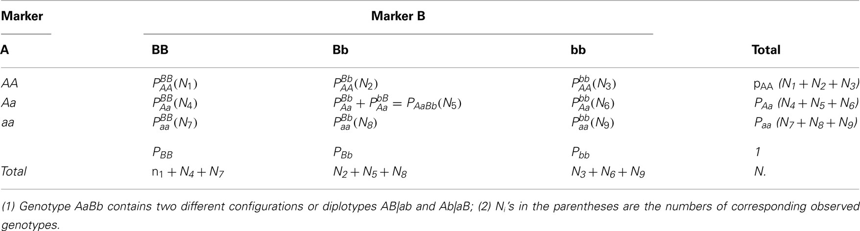
Table 1. Frequencies and numbers of observations of marker genotypes.

The two markers form four gametes, AB, Ab, aB, and ab, whose frequencies are denoted as p subscribed by the gamete notation. They are derived from diplotype frequencies by

\begin{array}{l} p_{A B} = P_{A A}^{B B} + \frac{1}{2} (P_{A A}^{B b} + P_{A a}^{B B} + P_{A a}^{B b}) \\ p_{A b} = P_{A A}^{b b} + \frac{1}{2} (P_{A A}^{B b} + P_{A a}^{b b} + P_{A a}^{b B}) \\ p_{a B} = P_{a a}^{B B} + \frac{1}{2} (P_{A a}^{B B} + P_{a a}^{B b} + P_{A a}^{b B}) \\ p_{a b} = P_{a a}^{b b} + \frac{1}{2} (P_{A a}^{b b} + P_{a a}^{B b} + P_{A a}^{B b}) . \end{array}

(4)

Similarly, the frequencies of non-alleles from different gametes are derived as

\begin{array}{l} p_{A / B} = P_{A A}^{B B} + \frac{1}{2} (P_{A A}^{B b} + P_{A a}^{B B} + P_{A a}^{b B}) \\ p_{A / b} = P_{A A}^{b b} + \frac{1}{2} (P_{A A}^{B b} + P_{A a}^{b b} + P_{A a}^{B b}) \\ p_{a / B} = P_{a a}^{B B} + \frac{1}{2} (P_{A a}^{B B} + P_{a a}^{B b} + P_{A a}^{B b}) \\ p_{a / b} = P_{a a}^{b b} + \frac{1}{2} (P_{A a}^{b b} + P_{a a}^{B b} + P_{A a}^{b B}) . \end{array}

(5)

In Eqs 4 and 5, diplotype frequencies $P_{A a}^{B b}$ and $P_{A a}^{b B}$ are mixed as a genotype frequency P_AaBb.

The frequencies of triple alleles from different markers are derived as

\begin{matrix} p_{A A}^{B} = P_{A A}^{B B} + \frac{1}{2} P_{A A}^{B b}, & p_{A A}^{b} = P_{A A}^{b b} + \frac{1}{2} P_{A A}^{B b} \\ p_{A a}^{B} = P_{A a}^{B B} + \frac{1}{2} (P_{A a}^{B b} + P_{A a}^{b B}), & p_{A a}^{b} = P_{A a}^{b b} + \frac{1}{2} (P_{A a}^{B b} + P_{A a}^{b B}) \\ p_{a a}^{B} = P_{a a}^{B B} + \frac{1}{2} P_{a a}^{B b}, & p_{a a}^{b} = P_{a a}^{b b} + \frac{1}{2} P_{a a}^{B b} \\ p_{A}^{B B} = P_{A A}^{B B} + \frac{1}{2} P_{A a}^{B B}, & p_{a}^{B B} = P_{a a}^{B B} + \frac{1}{2} P_{A a}^{B B} \\ p_{A}^{B b} = P_{A A}^{B b} + \frac{1}{2} (P_{A a}^{B b} + P_{A a}^{b B}), & p_{a}^{B b} = P_{a a}^{B b} + \frac{1}{2} (P_{A a}^{B b} + P_{A a}^{b B}) \\ p_{A}^{b b} = P_{A A}^{b b} + \frac{1}{2} P_{A a}^{b b}, & p_{a}^{b b} = P_{a a}^{b b} + \frac{1}{2} P_{A a}^{b b} . \end{matrix}

(6)

As shown above, all the genotype, allele, gamete, and non-gamete frequencies are uniquely determined by the diplotype frequencies. According to Table 1, the frequencies of all the diplotypes, except for AB|ab and Ab|aB, can be estimated from the observed data, since they are all one to one corresponding to genotypes which can be directly estimated from data.

A Complete Set of Disequilibria

Zygotic disequilibrium is defined as the deviation of two-locus genotype frequencies from products of single-locus genotype frequencies and, thus, is composed of all non-allelic genic disequilibria at the two loci (Weir, 1996). For a population at HWD, the desirable property of an equilibrium population will not occur, such as independence of different alleles at the same locus (Lynch and Walsh, 1998). The HWD attempts to test for two alleles at the same locus, but on different gametes, whereas (gametic) linkage disequilibrium describes two alleles on the same gametes, but at different loci. For a zygotic disequilibrium, however, there is a third test, i.e., two alleles on different gametes and at different loci.

Since the population is not in HWE, two alleles at each marker are not independent, with the coefficients of HWD defined as

\begin{array}{l} D_{A} = P_{A A} - p_{A}^{2} \\ = - \frac{1}{2} P_{A a} + p_{A} p_{a} \\ = P_{a a} - p_{a}^{2} \end{array}

(7)

for marker A and

\begin{array}{l} D_{B} = P_{B B} - p_{B}^{2} \\ = - \frac{1}{2} P_{B b} + p_{B} p_{b} \\ = P_{b b} - p_{b}^{2} \end{array}

(8)

for marker B, respectively. The coefficient of digenic gametic linkage disequilibrium between the two markers is defined as

\begin{array}{l} D_{a b} = p_{A B} - p_{A} p_{B} \\ = - p_{A b} + p_{A} p_{b} \\ = - p_{a B} + p_{a} p_{B} \\ = p_{a b} + p_{a} p_{b} . \end{array}

(9)

For the non-equilibrium population, digenic linkage disequilibrium that occurs between non-alleles at different gametes is defined as

\begin{array}{l} D_{a / b} = p_{A / B} - p_{A} p_{B} \\ = - p_{A / b} - p_{A} p_{b} \\ = - p_{a / B} - p_{a} p_{B} \\ = p_{a / b} - p_{a} p_{b} . \end{array}

(10)

The trigenic disequilibria between two alleles from marker A and one allele from marker B is defined as

\begin{array}{l} D_{A b} = p_{A A}^{B} - p_{A} D_{a b} - p_{A} D_{a / b} - p_{B} D_{A} - p_{A}^{2} p_{B} \\ = - p_{A A}^{b} - p_{A} D_{a b} - p_{A} D_{a / b} + p_{b} D_{A} + p_{A}^{2} p_{b} \\ = - \frac{1}{2} p_{A a}^{B} - \frac{1}{2} (p_{A} - p_{a}) D_{a b} - \frac{1}{2} (p_{A} - p_{a}) D_{a / b} \\ - p_{B} D_{A} + p_{A} p_{a} p_{B} \\ = p_{a a}^{B} + p_{a} D_{a b} - p_{a} D_{a / b} - p_{B} D_{A} - p_{a}^{2} p_{B} \\ = - p_{a a}^{b} + p_{a} D_{a b} - p_{a} D_{a / b} - p_{b} D_{A} - p_{a}^{2} p_{b} \end{array}

(11)

The trigenic disequilibria between one allele from marker A and two alleles from marker B is defined as

\begin{array}{l} D_{a B} = p_{A}^{B B} - p_{B} D_{a b} - p_{B} D_{a / b} - p_{A} D_{B} - p_{A} p_{B}^{2} \\ = - p_{a}^{B B} - p_{B} D_{a b} - p_{B} D_{a / b} + p_{a} D_{B} + p_{a} p_{B}^{2} \\ = - \frac{1}{2} p_{A}^{B b} - \frac{1}{2} (p_{B} - p_{b}) D_{a b} \\ - \frac{1}{2} (p_{B} - p_{b}) D_{a / b} - p_{a} D_{A} + p_{a} p_{B} p_{b} \\ = - \frac{1}{2} p_{a}^{B b} - \frac{1}{2} (p_{B} - p_{b}) D_{a b} \\ - \frac{1}{2} (p_{B} - p_{b}) D_{a / b} - p_{a} D_{A} + p_{a} p_{B} p_{b} \\ = p_{A}^{b b} + p_{b} D_{a b} + p_{b} D_{a / b} - p_{A} D_{A} - p_{A} p_{b}^{2} \\ = - p_{a}^{b b} + p_{b} D_{a b} + p_{b} D_{a / b} + p_{a} D_{A} + p_{a} p_{b}^{2} \end{array}

(12)

With diplotype frequencies, allele frequencies, HWD, gametic and non-gamete disequilibria, and trigenic disequilibria, we can derived the quadrigenic disequilibrium () between two alleles from marker A and two alleles from marker B (Weir, 1996). Analogous to Liu et al. (2006), we use a table (Table 2) to express the formulas for D_AB, from which it is clear that a full set of disequilibria can only be estimated from diplotype frequencies. In this article, D_AB will be estimated by using information from offspring genotypes. For clarity, we use small and capital letters to denote gamete and zygotic disequilibria, respectively. Conversely from Table 2, we can see that each of the diplotype frequencies can be expressed in terms of the allele frequencies (p_A, p_a and p_B, p_b), HWD coefficients (D_A and D_B) and gametic (D_ab) and non-gametic disequilibria of different orders (D_a/b, D_Ab, D_aB, and D_AB).

TABLE 2

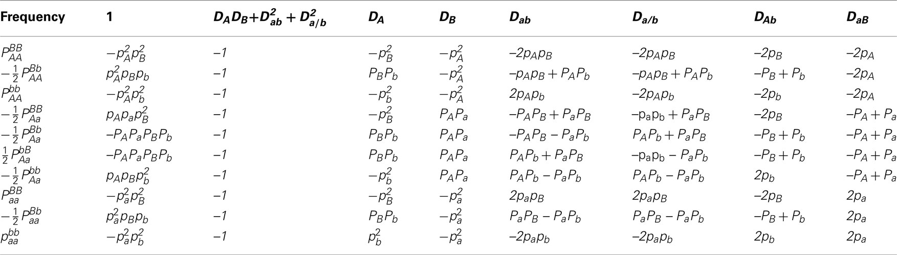
Table 2. Expressions of quadrigenic disequilibrium D_AB in terms of genotypic configuration frequencies, allele frequencies and lower-order disequilibrium coefficients.

Model for Estimation

Based on the above description, it can be seen that the estimation of all disequilibrium parameters purely relies on the separation of two diplotypes underlying the double heterozygote, since all the other diplotypes are one to one corresponding to their genotypes and can be directly estimated from the data. In this section, we show that these two diplotypes can be separated using an open-pollinated (OP) design. For a monoecious plant, each plant may be OP randomly by both its own pollen and that from the natural pool. In a dioecious plant, a female plant is only pollinated by the pollen pool. To simplify our explanation, we focus on dioecious plants. A model for monoecious plants will be described elsewhere.

Let N_i denote the number of maternal plants which bear on genotype i (i = 1,…,9) for the two SNPs considered and $N_{i}^{(j)}$ denote the number of offspring which have genotype j (j = 1,…,9) derived from maternal genotype i. Table 3 gives the structure of genotypic data collected from $N . = \sum_{i = 1}^{9} N_{i}$ random maternal plants and $N .^{(.)} = \sum_{i = 1}^{9} \sum_{j = 1}^{9} N_{i}^{(j)}$ random offspring plants, respectively. For a given maternal genotype, a certain group of offspring genotypes is produced. Table 4 gives genotype frequencies of offspring produced by any maternal genotype. For the OP design of dioecious plants, offspring genotypes are determined jointly by maternal gametes of the corresponding maternal plant and paternal gametes from the pollen pool. In the natural population, the frequencies of paternal gametes are expressed as p_AB, p_Ab, p_aB, and p_ab, respectively, which can be estimated from genotypic configuration frequencies by Eq. 4.

TABLE 3

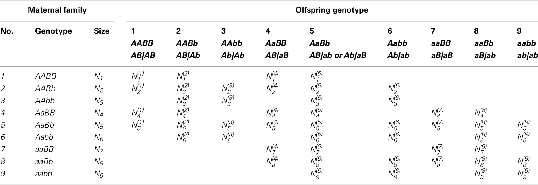
Table 3. Data structure of two markers in the OP design.

TABLE 4

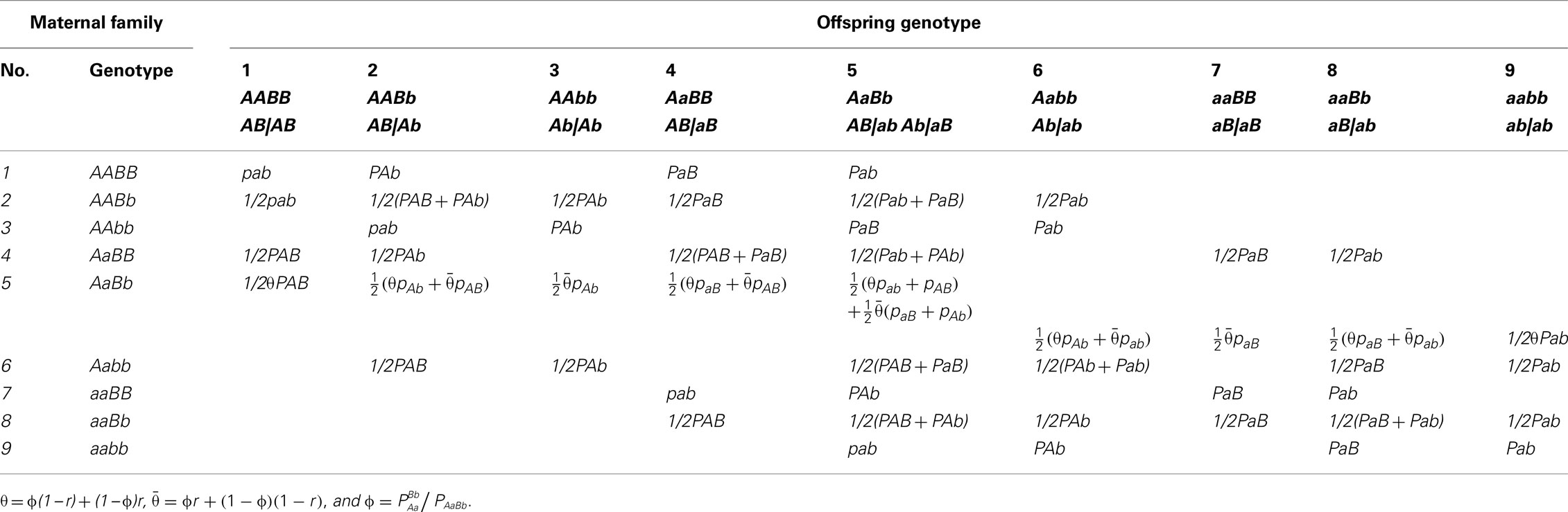
Table 4. Offspring genotype frequencies given each maternal genotype in the OP design.

The frequencies of maternal gametes are dependent on the genotype of a maternal plant. If the maternal plant is a double heterozygote AbBb, then any genotype generated in the offspring will include a mixture of genotypes derived from gametes of the two underlying diplotypes of the double heterozygote. The proportions of mixture components are determined by two parameters, the recombination fraction (r) between the two markers, and the relative proportions (ϕ) of the two underlying diplotypes to the double heterozygote. For a maternal plant with genotype AbBb, there are two possible diplotypes, AB|ab or Ab|aB, with relative frequencies

ϕ = \frac{P_{A a}^{B b}}{P_{A a B b}}, 1 - ϕ = \frac{P_{A a}^{b B}}{P_{A a B b}}

(13)

where P_AaBb is the frequency of the double heterozygote. Based on the definition of ϕ, we rewrite Eq. 4 to calculate the paternal gamete frequencies by

\begin{array}{l} p_{A B} = P_{A A}^{B B} + \frac{1}{2} (P_{A A}^{B b} + P_{A a}^{B B} + ϕ P_{A a B b}) \\ p_{A b} = P_{A A}^{b b} + \frac{1}{2} (P_{A A}^{B b} + P_{A a}^{b b} + (1 - ϕ) P_{A a B b}) \\ p_{a B} = P_{a a}^{B B} + \frac{1}{2} (P_{A a}^{B B} + P_{a a}^{B b} + (1 - ϕ) P_{A a B b}) \\ p_{a b} = P_{a a}^{b b} + \frac{1}{2} (P_{A a}^{b b} + P_{a a}^{B b} + ϕ P_{A a B b}) . \end{array}

(14)

Maternal diplotypes, AB|ab or Ab|aB, will produce four different maternal gametes, with relative frequencies depending on the recombination fraction (r) between the two markers:

yes

where we define θ = ϕ(1 − r) + r(1 − ϕ) and 1 − θ = ϕr + (1 − r)(1 − ϕ). Thus, overall haplotype frequencies produced by the double heterozygote maternal are calculated as $\frac{1}{2} θ$ for AB or ab and $\frac{1}{2} θ$ for Ab and aB.

As seen from Table 4, the conditional genotype frequencies of offspring given maternal genotypes depend on parameter θ and paternal gamete frequencies. Since paternal gamete frequencies (14) are determined by unknown parameter ϕ and genotype/diplotype frequencies estimated from maternal genotypes (which can be thought of constants), these conditional probabilities are actually dependent on only θ and ϕ.

Parameter Estimation with the MCMC Algorithm

As have been clear above, only two parameters ϕ and θ determine the genotype frequencies of offspring (Table 4). The log-likelihood of a complete set of genotype data includes the two parts based on the maternal and offspring genotypes, respectively, expressed as

\log L (ϕ, θ) = \log L_{M} (ϕ) + \log L_{0} (ϕ, θ) .

(16)

We have

\log L_{M} (ϕ) ∝ N_{1} \log P_{A A B B} + \dots + N_{5} \log P_{A a B b} + \dots + N_{9} \log P_{a a b b}

(17)

for the upper level of the log-likelihood that specifies the genotype distribution of maternal plants in the natural population, and

\begin{array}{l} \log L_{0} (ϕ, θ) \propto \\ + N_{1}^{(1)} \log p_{A B} + N_{1}^{(2)} \log p_{A b} + N_{1}^{(4)} \log p_{a B} + N_{1}^{(5)} \log p_{a b} \\ + \dots \\ + N_{5}^{(1)} \log (\frac{1}{2} θ p_{A B}) + N_{5}^{(2)} \log [\frac{1}{2} (θ p_{A b} + (1 - θ) p_{A B})] \\ + N_{5}^{(3)} \log [\frac{1}{2} (1 - θ) p_{A b}] \\ + N_{5}^{(4)} \log [\frac{1}{2} (θ p_{a B} + (1 - θ) p_{A B})] + N_{5}^{(5)} \log [\frac{1}{2} θ (P_{A B} + p_{a b}) \\ + \frac{1}{2} (1 - θ) (P_{A b} + P_{a B})] \\ + N_{5}^{(6)} \log [\frac{1}{2} (θ p_{A b} + (1 - θ) p_{a b})] + N_{5}^{(7)} \log [\frac{1}{2} (1 - θ) p_{a B}] \\ + N_{5}^{(8)} \log [\frac{1}{2} (1 - θ) p_{a B} + θ P_{a b}] \\ + N_{5}^{(9)} \log (\frac{1}{2} θ p_{a b}) \\ + \dots \\ + N_{9}^{(5)} \log p_{A B} + N_{9}^{(6)} \log p_{A b} + N_{9}^{(8)} \log p_{a B} + N_{9}^{(9)} \log p_{a b} \end{array}

(18)

for the lower level of the log-likelihood that specifies the transmission of alleles from parents to offspring.

Since all the genotype frequencies of maternal plants can be directly estimated by the observed data, we can view the upper level of the log-likelihood as constant, thus only focus on the lower level logL₀(ϕ,θ), i.e., logL(ϕ,θ)∝logL₀(ϕθ). Furthermore, logL₀(ϕ,θ) can be simplified as

\begin{array}{l} \log L_{0} (ϕ, θ) \\ \propto m_{1} \log p_{A B} + m_{2} \log p_{A b} + m_{3} \log p_{a B} + m_{4} \log p_{a b} \\ + m_{5} \log θ + m_{6} \log (1 - θ) + \\ + m_{7} \log [θ p_{a b} + (1 - θ) p_{A B}] + m_{8} \log [θ p_{a B} + (1 - θ) p_{A B}] \\ + m_{9} \log [θ p_{A b} + (1 - θ) p_{a b}] + m_{10} \log [θ p_{a B} + (1 - θ) p_{a b}] \\ + m_{11} \log [θ (p_{A B} + p_{a b}) + (1 - θ) (p_{A b} + p_{a B})] . \end{array}

where

\begin{array}{l} m_{1} = N_{1}^{(1)} + N_{2}^{(1)} + N_{3}^{(2)} + N_{4}^{(1)} + N_{5}^{(1)} + N_{6}^{(2)} + N_{7}^{(4)} \\ + N_{8}^{(4)} + N_{9}^{(5)}, \\ m_{2} = N_{1}^{(2)} + N_{2}^{(3)} + N_{3}^{(3)} + N_{4}^{(2)} + N_{5}^{(3)} + N_{6}^{(3)} + N_{7}^{(5)} \\ + N_{8}^{(6)} + N_{9}^{(6)}, \\ m_{3} = N_{1}^{(4)} + N_{2}^{(4)} + N_{3}^{(5)} + N_{4}^{(7)} + N_{5}^{(7)} + N_{6}^{(8)} + N_{7}^{(7)} \\ + N_{8}^{(7)} + N_{9}^{(8)}, \\ m_{4} = N_{1}^{(5)} + N_{2}^{(6)} + N_{3}^{(6)} + N_{4}^{(8)} + N_{5}^{(9)} + N_{6}^{(9)} + N_{7}^{(8)} \\ + N_{8}^{(9)} + N_{9}^{(9)}, \\ m_{5} = N_{5}^{(1)} + N_{5}^{(9)}, m_{6} = N_{5}^{(3)} + N_{5}^{(7)}, \\ m_{7} = N_{5}^{(2)}, m_{8} = N_{5}^{(4)}, m_{9} = N_{5}^{(6)}, \\ m_{10} = N_{5}^{(8)}, m_{11} = N_{5}^{(5)} . \end{array}

(19)

Therefore, the posterior distribution of ϕ and θ based on all the other information can be obtained, respectively, by

\begin{array}{l} \log π (ϕ | θ, N) \\ \propto m_{1} \log p_{A B} + m_{2} \log p_{A b} + m_{3} \log p_{a B} + m_{4} \log p_{a b} \\ + m_{7} \log [θ p_{A b} + (1 - θ) p_{A B}] + m_{8} \log [θ p_{a B} + (1 - θ) p_{A B}] \\ + m_{9} \log [θ p_{A b} + (1 - θ) p_{a b}] + m_{10} \log [θ p_{a B} + (1 - θ) p_{a b}] \\ + m_{11} \log [θ (p_{A B} + p_{a b} + (1 - θ) (p_{A b} + p_{a B}))] . \end{array}

(20)

\begin{array}{l} \log π (ϕ | θ, N) \\ \propto m_{5} \log θ + m_{6} \log (1 - θ) + m_{7} \log [θ p_{A b} + (1 - θ) p_{A B}] \\ + m_{8} \log [θ p_{a B} + (1 - θ) p_{A B}] + m_{9} \log [θ p_{A b} + (1 - θ) p_{a b}] \\ + m_{10} \log [θ p_{a B} + (1 - θ) p_{a b}] + m_{11} \log [θ (p_{A B} + p_{a b}) \\ + (1 - θ) (p_{A b} - p_{a B})] . \end{array}

(21)

Notice that p_AB, p_Ab, p_aB, and p_ab are a function of ϕ according to equation (14). Then, within the Bayesian framework, the MCMC technique can be used to draw samples from the posterior distributions of ϕ and θ. We will use the Variable-at-a-Time Metropolis-Hastings algorithm described as follows:

1) Start with initial value (ϕ⁽⁰⁾,θ⁽⁰⁾);

2) After getting (ϕ⁽ⁿ⁾,θ⁽ⁿ⁾), update ϕ from ϕ⁽ⁿ⁾ to ϕ⁽ⁿ⁺¹⁾ according to logπ(ϕ|θ⁽ⁿ⁾,N) using proposal Unif(0,1): Generate ϕ* from Unif(0,1) and accept it, i.e., set ϕ⁽ⁿ⁺¹⁾ = ϕ* with probability α, where logα = min{0,logπ(ϕ*|θ⁽ⁿ⁾,N) − logπ(ϕ⁽ⁿ⁾|θ⁽ⁿ⁾,N)}; otherwise, set ϕ⁽ⁿ⁺¹⁾ = ϕ⁽ⁿ⁾;

3) After getting (ϕ⁽ⁿ⁺¹⁾ = θ⁽ⁿ⁾), update θ from θ⁽ⁿ⁾ to θ⁽ⁿ⁺¹⁾ according to logπ(θ|ϕ⁽ⁿ⁺¹⁾,N) using proposal Unif(0,1): Generate θ* from Unif(0,1) and accept it, i.e., set θ⁽ⁿ⁺¹⁾ = θ* with probability β, where logβ = min{0,logπ(θ_*|ϕ⁽ⁿ⁺¹⁾,N)− logπ(θ⁽ⁿ⁾|ϕ⁽ⁿ⁺¹⁾,N)}; otherwise, set θ⁽ⁿ⁺¹⁾ = θ⁽ⁿ⁾;

4) Repeat (2) and (3) n times, where n is the number of iterations.

5) After burning in the first few sampled ϕ and θ, get the mean values of the remaining samples as the respective estimates. The estimate of r can be obtained by

r = \frac{θ - ϕ}{1 - 2 ϕ} from θ = ϕ (1 - r) + r (1 - ϕ) .

Since the values of r, ϕ and, hence, θ have restricted domains as follows:

0 \leq r \leq 0.5; 0 \leq ϕ \leq 1; 0 \leq θ \leq 1,

we choose Uniform (0,1) as a proposal distribution when updating both ϕ and θ.

With the estimate of ϕ, we can separate two diplotypes of the double heterozygote. Therefore, all the frequencies and disequilibria are obtained from Eqs 1 to 12 and Table 2. Also, we provide an estimate of the recombination fraction.

Computer Simulation

The statistical properties of the new model were investigated through simulation studies. The values of zygotic disequilibria used to simulate marker data for the OP design were chosen from their spaces which were shown in Liu et al. (2006). Because of the limitation of a population-based sampling design, Liu et al. (2006) was not able to estimate all types of zygotic disequilibria. By collapsing gametic and non-gametic linkage disequilibria, leading to a composite quadrigenic disequilibrium rather than the quadrigenic disequilibrium as defined in Table 2, they provided a reduced model for disequilibrium analyses. In a comparison with the traditional gametic linkage disequilibrium model, Liu et al.’s reduced model was found to be more general and cover the results from the former. It is expected that our model covers Liu et al.’s model because we do not need to combine gametic and non-gametic linkage disequilibria.

The simulation uses three different scenarios. The first assumes different relative proportions of two diplotypes for the double heterozygote (ϕ) by fixing the recombination fraction. In order to obtain different ϕ values, we need to adjust the zygotic disequilibria. Specifically, we have three combinations:

(1) ϕ = 0.87 and D_ab= 0.1, D_a/b= D_Ab= D_aB= D_AB= 0.01

(2) ϕ = 0.12 and D_a/b= 0.1, D_ab= D_Ab= D_aB= D_AB= 0.01

(3) ϕ = 0.5 and D_ab= D_a/b= 0.02, D_Ab= D_aB= 0.03, D_AB= 0.01,

in which r = 0.2, p_A= 0.5, p_B= 0.6, D_A= D_B= 0.05, and the true value of θ can be calculated given ϕ and r by equation (15). The second is to change the recombination fraction, i.e., (1) r = 0.3, (2) r = 0.05, and (3) r = 0.5, with the other parameters fixed, i.e., ϕ = 0.87, p_A= 0.5, p_A= 0.6, D_A= D_B= 0.05, D_ab= 0.01, D_a/b= D_Ab= D_aB= D_AB= 0.01. The third is about sampling strategies, (1) 1000 maternal plants × 9 seeds per family and (2) 200 maternal plants × 49 seeds per family, producing the same total size of samples, in which ϕ = 0.87, r = 0.2, p_A= 0.5, p_B= 0.6, D_A= D_B= 0.05, D_ab= 0.1, D_a/b= D_Ab= D_aB= D_AB= 0.01. For the first two scenarios, we use 1000 × 9 strategy.

For the simulated data, we estimated all genotype frequencies from maternal genotype data, which were used to estimate p_A, p_B, D_A, D_B, D_Ab, and D_aB with equations (1), (2), (3), (6), (7), (8), (11), and (12), respectively. However, D_ab, D_a/b, and D_AB can be estimated only after ϕ is estimated. Tables 5–7 give the results from simulated data under three different scenarios. In each case, 1000 simulation replicates were performed to get the means and standard deviations of the estimates. Each estimate was based on 1000 iterations after burns-in during the MCMC procedure. In general, all parameters can be estimated reasonably from our model.

TABLE 5

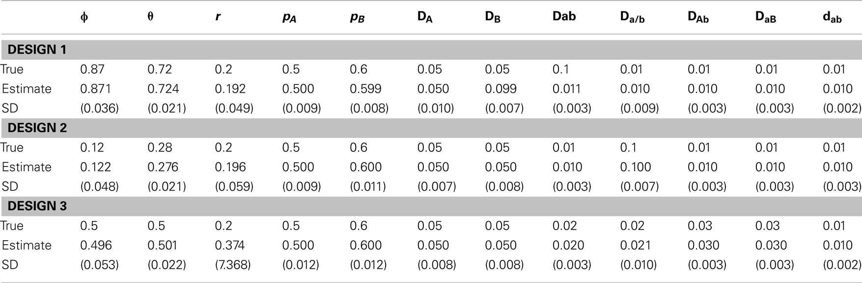
Table 5. Estimates of parameters and their standard deviations (in parentheses) based on the MCMC algorithm for the data simulated under scenario 1.

In scenario 1, uneven allocations of two diplotypes for the double heterozygote help the estimates of the recombination fraction (Table 5). If these two diplotypes are equally allocated, i.e., ϕ = 0.5, we could not give a good estimate of the recombination fraction because in this case θ is not dependent on r, making r unidentifiable. As shown in Li and Wu (2009), a three-locus analysis can overcome this problem. In scenario 2, we found that ϕ and all set of disequilibria can be precisely estimated, no matter whether r = 0.5 or not (Table 6). This is because the MCMC procedure treats ϕ and θ as two separate parameters. The results of scenario 3 help to determine an optimal sampling strategy. As expected, sampling more maternal plants increases the precision of parameter estimation (Table 7).

TABLE 6

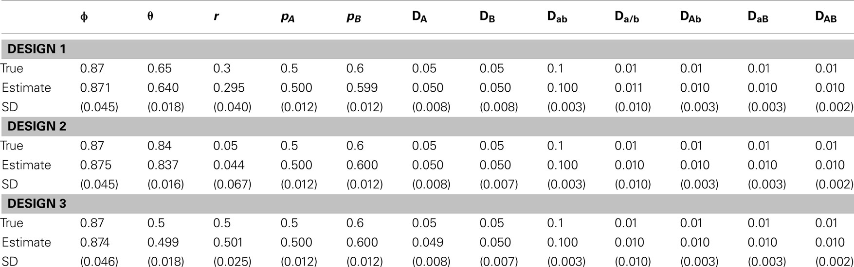
Table 6. Estimates of parameters and their standard deviations (in parentheses) based on the MCMC algorithm for the data simulated under scenario 2.

TABLE 7

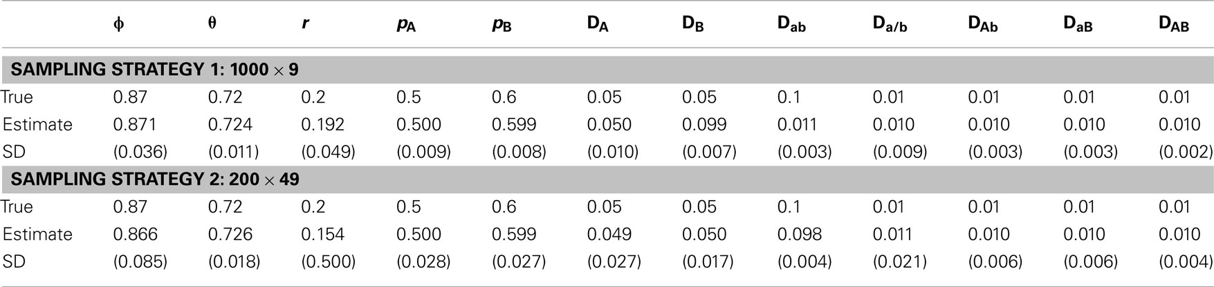
Table 7. Estimates of parameters and their standard deviations (in parentheses) based on the MCMC algorithm for the data simulated under scenario 3.

Discussion

The structural study of linkage disequilibrium helps to understand the genetic variation and evolution of populations and facilitates the positional cloning of genes underlying common complex diseases (Lewontin, 1964, 1988; Hedrick, 1987; Weir, 1996; Kruglyak, 1999). The current approaches for estimating linkage disequilibria rely on the assumption that the population under consideration is randomly mating, following Hardy–Weinberg equilibrium (HWE). However, many populations may be founded by a small number of ancestors and/or are frequently under evolutionary pressure, such as mutation, genetic drift, population admixture, and structure (Lynch and Walsh, 1998). For those populations, HWE may be violated. We need a new analysis that relaxes the random mating assumption. Weir (1996) introduced the concept of zygotic association or zygotic disequilibrium that specify the disequilibria between different loci in a non-equilibrium population. Part of these disequilibria was used by Liu et al. (2006) to examine the extent and distribution of zygotic disequilibria across the canine genome.

In this article, we have for the first time developed a new statistical model for estimating a complete set of zygotic disequilibria, including (1) Hardy–Weinberg disequilibria at each locus, (2) gametic disequilibrium (including two alleles in the same gamete, each from a different locus), (3) non-gametic disequilibrium (including two alleles in different gametes, each from a different locus), (4) trigenic disequilibrium (including a zygote at one locus and an allele at the other), and (5) quadrigenic disequilibrium (including two zygotes each from a different locus). This model is based on an open-pollinated (OP) design by sampling multiple maternal plants and their offspring. The major advantage of this design lies in its power to separate two diplotypes of a double heterozygote (specified by a proportion ϕ), thus retrieving the lost information of a traditional population-based sampling strategy.

Under the OP design setting, a full log-likelihood of diplotype frequencies from the maternal and offspring generations was formulated in terms of two unique parameters, ϕ and recombination fraction r. An MCMC procedure was then implemented to estimate these two parameters from which a full set of zygotic disequilibria and the recombination fraction are estimated. Extensive simulation studies have been performed to test the statistical behavior of the new model by considering a range of disequilibrium and recombination fraction as well as different sampling strategies. In general, all the parameters can be estimated with reasonable accuracy and precision.

As a first attempt to relax the Hardy–Weinberg equilibrium assumption that has been widely accepted for population genetic studies of many decades, our model will reshape the fundamental theory of this field. With an increasing availability of genetic data due to the rapid development of genotyping technologies, this model will show its increasing implications and likelihood for uncovering new discoveries related to population genetics. The model can be extended to accommodate various situations in the following aspects. First, by integrating selfing rates into the model, we can develop a similar design for monoecious plants in which the simultaneous occurrence of female and male flowers allows selfing. Second, a multilocus model including more than two markers should be developed. This will not only increase the power of the model by estimating genetic interference, but also overcome the problem of estimating the recombination fraction when ϕ is equal to 0.5. Third, the model can be integrated with quantitative traits to map their underlying QTLs and genetic interactions (see Wu et al., 2002). All these extensions will make our model more useful in practice, ultimately resolving difficult challenges in population and quantitative genetic studies.

Conflict of Interest Statement

The authors declare that the research was conducted in the absence of any commercial or financial relationships that could be construed as a potential conflict of interest.

Acknowledgments

This work is partially supported by NSF/IOS-0923975 to Rongling Wu and NIDA, NIH grants R21 DA024260 and R21 DA024266 to Runze Li. The content is solely the responsibility of the authors and does not necessarily represent the official views of the NIDA or the NIH.

References

Barton, N. H., and Gale, K. S. (1993). “Genetic analysis of hybrid zones,” in Hybrid Zones and the Evolutionary Process, eds R. G. Harrison and J. Price (Oxford: Oxford University Press), 13–45.

Bennett, J. H., and Binet, F. E. (1956). Association between Mendelian factors with mixed selfing and random mating. Heredity 10, 51–55.

CrossRef Full Text

Charlesworth, B. (1991). The evolution of sex chromosomes. Science 251, 1030–1033.

Pubmed Abstract | Pubmed Full Text | CrossRef Full Text

Haldane, J. B. S. (1949). The association of characters as a result of inbreeding and linkage. Ann. Eugen. 15, 15–23.

Pubmed Abstract | Pubmed Full Text | CrossRef Full Text

Hedrick, P. W. (1987). Gametic disequilibrium measures: proceed with caution. Genetics 117, 331–341.

Pubmed Abstract | Pubmed Full Text

Hou, W., Liu, T., Li, Y., Li, Q., Li, J. H., Das, K., and Wu, R. L. (2009). Multilocus genomics of outcrossing populations. Theor. Popul. Biol. 76, 68–76.

Pubmed Abstract | Pubmed Full Text | CrossRef Full Text

Kruglyak, L. (1999). Prospects for whole-genome linkage disequilibrium mapping of common disease genes. Nat. Genet. 22, 139–144.

Pubmed Abstract | Pubmed Full Text | CrossRef Full Text

Lewontin, R. C. (1964). The interaction of selection and linkage. General considerations, heterotic models. Genetics 49, 49–67.

Pubmed Abstract | Pubmed Full Text

Lewontin, R. C. (1988). On measures of gametic disequilibrium. Genetics 120, 849–852.

Pubmed Abstract | Pubmed Full Text

Li, J. H., Li, Q., Hou, W., Han, K., Li, Y., Wu, S., Li, Y. C., and Wu, R. L. (2009). An algorithmic model for constructing a linkage and linkage disequilibrium map in open-pollinated progeny populations. Genet. Res. 91, 9–21.

CrossRef Full Text

Li, Q., and Wu, R. L. (2009). A multilocus model for constructing a linkage disequilibrium map in human populations. Stat. Appl. Genet. Mol. Biol. 8, article 18.

Li, Y., Li, Y., Wu, S., Han, K., Wang, Z., Hou, W., Zeng, Y., and Wu, R. (2007). Estimation of multilocus linkage disequilibria in diploid populations with dominant markers. Genetics 176, 1811–1821.

Pubmed Abstract | Pubmed Full Text | CrossRef Full Text

Liu, T., Todhunter, R. J., Lu, Q., Schoettinger, L., Li, H. Y., Littell, R. C., Bliss, S., Acland, G., Lust, G., and Wu, R. L. (2006). Extent and distribution of zygotic linkage disequilibrium in canine. Genetics 174, 439–453.

Pubmed Abstract | Pubmed Full Text | CrossRef Full Text

Lou, X. Y., Casella, G., Littell, R. C., Yang, M. C. K., Johnson, J. A., and Wu, R. L. (2003). A haplotype-based algorithm for multilocus linkage disequilibrium mapping of quantitative trait loci with epistasis. Genetics 163, 1533–1548.

Pubmed Abstract | Pubmed Full Text

Lynch, M., and Walsh, B. (1998). Genetics and Analysis of Quantitative Traits. Sunderland, MA: Sinauer Associates.

Slatkin, M. (2008). Linkage disequilibrium – understanding the evolutionary past and mapping the medical future. Nat. Rev. Genet. 9, 477–485.

Pubmed Abstract | Pubmed Full Text | CrossRef Full Text

Weir, B. (1996). Genetic Data Analysis II. Sunderland, MA: Sinauer Associates.

Wu, R. L., Ma, C. X., and Casella, G. (2002). Joint linkage and linkage disequilibrium mapping of quantitative trait loci in natural populations. Genetics 160, 779–792.

Pubmed Abstract | Pubmed Full Text

Wu, R. L., and Zeng, Z. B. (2001). Joint linkage and linkage disequilibrium mapping in natural populations. Genetics 157, 899–909.

Pubmed Abstract | Pubmed Full Text

Wu, S., Yang, J., and Wu, R. L. (2010). Mapping quantitative trait loci in a non-equilibrium population. Stat. Appl. Genet. Mol. Biol. 9, article 32.

Yang, R. C. (2000). Zygotic associations and multilocus statistics in a nonequilibrium diploid population. Genetics 155, 1449–1458.

Pubmed Abstract | Pubmed Full Text

Yang, R. C. (2002). Analysis of multilocus zygotic associations. Genetics 161, 435–445.

Pubmed Abstract | Pubmed Full Text

Keywords: gametic linkage disequilibrium, zygotic linkage disequilibrium, Hardy–Weinberg equilibrium, non-equilibrium population, molecular marker

Citation: Liu J, Wang Z, Wang Y, Li R and Wu R (2012) Model and algorithm for linkage disequilibrium analysis in a non-equilibrium population. Front. Gene. 3:78. doi: 10.3389/fgene.2012.00078

Received: 30 September 2011; Paper pending published: 31 October 2011;
Accepted: 24 April 2012; Published online: 02 July 2012.

Edited by:

Christina Kitchen, University of California Los Angeles, USA

Reviewed by:

Dalin Li, Cedars-Sinai Medical Center, USA
Christina Kitchen, University of California Los Angeles, USA

Copyright: © 2012 Liu, Wang, Wang, Li and Wu. This is an open-access article distributed under the terms of the Creative Commons Attribution Non Commercial License, which permits non-commercial use, distribution, and reproduction in other forums, provided the original authors and source are credited.

*Correspondence: Rongling Wu, Division of Biostatistics and Bioinformatics, Pennsylvania State University, Hershey, 17033 PA, USA. e-mail: rwu@hes.hmc.psu.edu

Disclaimer: All claims expressed in this article are solely those of the authors and do not necessarily represent those of their affiliated organizations, or those of the publisher, the editors and the reviewers. Any product that may be evaluated in this article or claim that may be made by its manufacturer is not guaranteed or endorsed by the publisher.