A Hierarchical Bayesian Approach to Multi-Trait Clinical Quantitative Trait Locus Modeling

Recent advances in high-throughput genotyping and transcript profiling technologies have enabled the inexpensive production of genome-wide dense marker maps in tandem with huge amounts of expression profiles. These large-scale data encompass valuable information about the genetic architecture of important phenotypic traits. Comprehensive models that combine molecular markers and gene transcript levels are increasingly advocated as an effective approach to dissecting the genetic architecture of complex phenotypic traits. The simultaneous utilization of marker and gene expression data to explain the variation in clinical quantitative trait, known as clinical quantitative trait locus (cQTL) mapping, poses challenges that are both conceptual and computational. Nonetheless, the hierarchical Bayesian (HB) modeling approach, in combination with modern computational tools such as Markov chain Monte Carlo (MCMC) simulation techniques, provides much versatility for cQTL analysis. Sillanpää and Noykova (2008) developed a HB model for single-trait cQTL analysis in inbred line cross-data using molecular markers, gene expressions, and marker-gene expression pairs. However, clinical traits generally relate to one another through environmental correlations and/or pleiotropy. A multi-trait approach can improve on the power to detect genetic effects and on their estimation precision. A multi-trait model also provides a framework for examining a number of biologically interesting hypotheses. In this paper we extend the HB cQTL model for inbred line crosses proposed by Sillanpää and Noykova to a multi-trait setting. We illustrate the implementation of our new model with simulated data, and evaluate the multi-trait model performance with regard to its single-trait counterpart. The data simulation process was based on the multi-trait cQTL model, assuming three traits with uncorrelated and correlated cQTL residuals, with the simulated data under uncorrelated cQTL residuals serving as our test set for comparing the performances of the multi-trait and single-trait models. The simulated data under correlated cQTL residuals were essentially used to assess how well our new model can estimate the cQTL residual covariance structure. The model fitting to the data was carried out by MCMC simulation through OpenBUGS. The multi-trait model outperformed its single-trait counterpart in identifying cQTLs, with a consistently lower false discovery rate. Moreover, the covariance matrix of cQTL residuals was typically estimated to an appreciable degree of precision under the multi-trait cQTL model, making our new model a promising approach to addressing a wide range of issues facing the analysis of correlated clinical traits.

Introduction

Integrating genetic polymorphism and gene expression data to elucidate the genetic architecture and regulatory networks of complex clinical traits is a rousing trend in modern biology. This tendency owes much to the now established view (e.g., Schadt et al., 2005; Kendziorski et al., 2006; Lee et al., 2009; Mackay, 2009) that gene expression profiles usually act as intermediate phenotypes between genetic polymorphism and the phenotypic traits of interest.

The genomic loci associated with the variation in gene transcript levels, known as expression quantitative trait loci (eQTLs), can be identified through a standard quantitative trait locus (QTL) mapping framework, with transcript levels acting as surrogate for classical quantitative traits (Jansen and Nap, 2001; Schadt et al., 2003; Cheung et al., 2005; Drake et al., 2006; Breitling et al., 2008). An expression profile that is treated as a continuous trait for mapping purposes is called an expression trait (eTrait; Zou et al., 2007), and the genome-wide genetic analysis of gene expression data is known as genetical genomics (Jansen and Nap, 2001) or transcriptome mapping (Li and Deng, 2010).

An eQTL is said to be cis- or trans-acting (Brem et al., 2002), depending on its location with regard to the chromosomal position of its target gene (i.e., the gene whose expression it regulates). A cis eQTL encompasses the genomic location of its target gene, whereas a trans eQTL maps to a distant genomic location. Trans eQTLs may aggregate in small segments of DNA sequences called genomic “hotspots” in which each eQTL may regulate a large number of gene transcripts (Breitling et al., 2008; Wu et al., 2008). It is, however, not straightforward to determine whether an eQTL acts in cis or in trans. One way out is to consider as cis-acting all eQTLs lying within a specific distance of their target genes, and view the ones that are far removed from their target genes as trans-acting (e.g., Brem et al., 2002; Wittkopp, 2005). Along these lines, Brem et al. (2002) used 10 kb as the threshold distance for distinguishing between cis- and trans-regulatory effects.

With the advent of high-throughput genotyping and transcript profiling technologies, it is now easy and inexpensive to concurrently generate genome-wide dense marker maps and huge amounts of expression profiles for each individual in a study population (Borevitz et al., 2003; Ronald et al., 2005). These large-scale data are generally littered with valuable information on the link between genetic polymorphisms and clinical traits of interest, and on the subtle molecular networks or pathways involved. The simultaneous utilization of marker and expression data to explain the variation in clinical quantitative traits is termed clinical quantitative trait locus (cQTL) analysis (Hoti and Sillanpää, 2006; Sillanpää and Noykova, 2008; Pikkuhookana and Sillanpää, 2009). cQTL analysis poses many problems and challenges, four of which are pointed out below.

(1) The high model dimensionality implied by the huge number of parameters undermines the effectiveness of standard statistical methods. (2) High correlations between predictors (markers or expressions) tend to reduce statistical power in the sense that, if one predictor shows a spurious association, its correlates will most likely show that same erroneous association. (3) The statistical issue of inflated false discovery rate (FDR) or type I error due to multiple testing (Kendziorski et al., 2006) limits the usefulness of single-locus testing procedures. A multi-locus approach provides more power for identifying the few potentially relevant loci to the phenotype-to-genotype association in both QTL and eQTL analyses. (4) Small sample size in terms of the number of individuals (de Koning and Haley, 2005) remains a problem in both QTL and eQTL analyses as the curse of dimensionality associated with the so-called “large p small n” problem is ever more ubiquitous. In this regard, regularization or shrinkage methods (e.g., Xu, 2003; Mutshinda and Sillanpää, 2010, 2011) are increasingly advocated as an effective way of reducing the model dimensionality in a regression set-up, by shrinking the effects of irrelevant covariates toward zero.

Hierarchical Bayesian (HB) modeling or Bayesian multilevel modeling (Gelman et al., 2003) provides a convenient approach for combining information from various data sources and accommodating uncertainty at different levels. By HB model, we understand a Bayesian model conceptualized in a hierarchical form in the sense that, the parameters involved in the likelihood function have priors, the parameters of which may also have priors involving a set of parameters, which may in turn have priors and so on, with the process coming to an end when no new priors are introduced (e.g., Mutshinda et al., 2008). In many cases, the HB prior specification provides the flexibility to define more realistic priors intended to match the requirements of the data at hand, while taking into account existing knowledge and expert opinion. It also helps enhance parameter estimation by “borrowing strength” from data used to estimate related quantities. With recent advances in computer intensive sampling-based methods such as Markov chain Monte Carlo (MCMC) simulation techniques (Gilks et al., 1996), the computational hurdles that have long prevented the broad application of HB modeling are no longer an issue; Bayesian models of arbitrary complexity are now being developed and implemented across a broad spectrum of scientific disciplines.

Sillanpää and Noykova (2008) developed a HB model for single-trait cQTL analysis in inbred line cross-data, using molecular markers, gene expressions, and marker-gene expression pairs. Their approach involved an eQTL model as missing data model for the intermediate link between markers and transcript levels in the determination of clinical phenotypic traits. The intermediate eQTL model can provide valuable insights into gene networks and molecular mechanisms linking genes to the clinical traits of interest.

It has, however, been pointed out (e.g., Mackay, 2009) that phenotypic traits do not exist in isolation; they often relate to one another through environmental correlations and pleiotropy. Many authors, including Jiang and Zeng (1995) and Liu et al. (2007, 2008) have pointed up a number of advantages of a joint analysis of multiple correlated traits over their separate analyses. These include the improvement on the statistical power to detect QTLs and on the precision of parameter estimation. Moreover, a multi-trait model provides a formal framework for examining a number of biologically interesting hypotheses regarding the underpinnings of genetic correlations between different traits. This understanding is crucial in animal and plant breeding where, as pointed out by Jiang and Zeng (1995), one of the major goals is to break unfavorable linkage.

The aim of this study is to extend the HB cQTL model for inbred line crosses proposed by Sillanpää and Noykova (2008) to a multi-trait setting, to illustrate the implementation or our new model with simulated the data, and evaluate its performance, using the single-trait counterpart as benchmark for comparison.

Materials and Methods

Description of the Input Data

Keeping with Sillanpää and Noykova (2008), we restrict attention to inbred line crosses such as backcross or double haploid progeny with one of two possible genotypes at any locus. However, the model can straightforwardly be adapted for the F₂ inter-cross design as discussed in the appendix of Sillanpää and Noykova (2008).

The input data involve molecular markers, gene expressions, and a set of clinical phenotypic traits of interests from each sampled individual. In addition, some marker-expression associations are a priori suggested for inclusion in the model, and may concern cis- or trans-regulatory effects. Hoti and Sillanpää (2006) refer to the marker-gene expression pairs as linked data. The linked data may result from oligonucleotide array data (Borevitz et al., 2003; Ronald et al., 2005) where markers and gene expression measurement are concurrently produced at every position, or be based on earlier findings of eQTL analyses or some known pathways. In cases where there is no a priori information to suggest the linked marker-expression pairs, these can be created from genetic distances, by assuming in cis effects between a marker and all genes falling within a specific genetic distance from it. As in Sillanpää and Noykova (2008), we assume each expression to be regulated by a single marker, without excluding the possibility for a marker to simultaneously regulate two or more expressions. In the latter case, the involved marker needs to be represented twice or as many times as required, the distance between its different copies being roughly zero.

Specification of the Multi-Trait cQTL Model

Let $y=\left[{\mathbf{\text{y}}}_1,{\mathbf{\text{y}}}_{\text{2}},\dots ,{\mathbf{\text{y}}}_{N_t}\right]$ denote the values of the N_t clinical quantitative traits of interest on the N study individuals, where y_k = (y_k,1, y_k,2, …, y_k,N)^T represents the measurements of the kth trait (k = 1…N_t). For each trait, the cQTL model of Sillanpää and Noykova (2008) is assumed. That is,

${\mathbf{\text{y}}}_k=a_k\mathbf{\text{1}}+\tilde{X}{\eta }_k+{\mathbf{\text{e}}}_k, (1)$

where a_k is the population intercept for the kth trait, 1 is the N × 1 vector of ones, e _k = (e_k,1, e_k,2, …, e_k,N)^T is the residual vector associated with the kth trait, and $\tilde{\text{X}}$ is the design matrix involving N_P markers (G), N_P expressions (E), and N_P marker-expression pairs (GE) organized as $\tilde{\text{X}}=\left[\text{G\hspace{0.17em}}\left|\text{\hspace{0.17em}E\hspace{0.17em}}\right|\text{\hspace{0.17em}GE}\right]$. The parameter vector η_k therefore, describes the regulatory effect of genetic data on the kth trait. The full multi-trait cQTL model can be compactly written as

$\mathbf{\text{y}}=\mathbf{\text{a}}+\mathbf{\text{X}}\eta +\mathbf{\text{e}}, (2)$

where $\mathbf{\text{a}}=\left(a_1\mathbf{\text{1}},a_2\mathbf{\text{1}},\dots ,a_{N_t}\mathbf{\text{1}}\right)$, X is a block-diagonal matrix comprising N_t blocks identical to $\widetilde{\mathbf{\text{X}}},\eta =\mathbf{\text{I}}\bullet \beta$ is the 3N_pN_t × 1 vector of regression coefficients to be estimated from the data, • denotes the entry-wise (Hadamard or Schur) product, I represents a 3N_pN_t × 1 vector of indicators, and β is the 3N_pN_t × 1 vector of genetic effects. As pointed out earlier, the method is developed for experimental crosses such as backcross or double haploid progeny with only one of two possible genotypes at any locus. Assuming that one genotype is coded as 1 and the other as −1, the size of the cQTL effects is represented by the quantity 2Iβ.

The regression terms η^M, η^E, and η^ME are respectively related to the marker genotypes, the expression measurements, and the mixed marker-expression pairs; $\mathbf{\text{e}}=\left({\mathbf{\text{e}}}_1,{\mathbf{\text{e}}}_2,\cdots ,{\mathbf{\text{e}}}_{N_t}\right)$ is the N_tN × 1 residual vector assumed to follow a multivariate normal distribution $e\sim MVN\left(\tilde{0},\text{S\hspace{0.17em}}\otimes {\text{I}}_N\right)$ with the N_tN × 1 vector $\widetilde{\mathbf{\text{0}}}={\left(0,0,\dots ,0\right)}^T$ as mean and a (N_t N × N_t N) covariance matrix Σ = S ⊗ I _N, where ⊗ denotes the Kronecker product operator. Here S is an N_t × N_t covariance matrix describing the variances and the (within individual) dependence between the residuals of different traits and I _N is the N × N identity matrix. This said, the distribution of y is given by y ∼ MVN(a + Xη, S ⊗ I _N), where a, X, and η are defined above.

Hierarchical Structure of the Multi-Trait cQTL Model

Our HB multi-trait cQTL model comprises four hierarchical levels as graphically depicted in Figure 1. Note that the intermediate eQTL model, presented as a shadowed box in the figure, is exactly the same as the eQTL part of the single-trait cQTL model (Sillanpää and Noykova, 2008). A detailed description of each hierarchical level is given below.

FIGURE 1

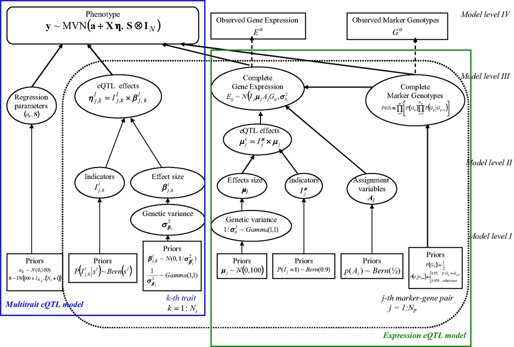
Figure 1. Hierarchical directed acyclic graph (DAG) of the model structure. The pre-specified values (Model level I) or observed data (Model level IV) are given in boxes. Ellipses (Model levels II and III) refer to the unknown random variables, which are sampled. The solid arrows illustrate hierarchical dependencies, and the dotted arrows show deterministic dependences. The box given in bold indicates the multi-trait model structure.

Model level IV

The highest level (level IV) of our HB model is represented by data vector D = (E⁰, G⁰, y).

Here the phenotypic data y (modeled by Eq. 1) for all N_t traits are assumed to be available with no missingness, while the observed gene expressions E^o and marker genotypes G^o may involve some missing values. The complete marker and expression data are respectively denoted by G and E.

The parameters θ = (θ^c, θ^e) to be estimated can be partitioned into two groups, namely θ^c = (I, β, a, S) = (η, a, S) which are directly involved in cQTL model (2), and ${\theta }^{\mathbf{\text{e}}}=\left(I^{\mu },\mu ,A,G,E,{\sigma }_0^2\right)$ used in the intermediate eQTL model. The eQTL model parameter ${\sigma }_0^2$ is the expression variance, I^μ is a vector of indicators, μ is the vector of eQTL effect sizes, and A comprises the assignment variables which, as in Sillanpää and Noykova (2008), define the expression eQTL regulatory effects of the marker-expression pairs.

According the Bayes theorem p(θ | D) ∝ p(D,θ) = p(D | θ)p(θ), which is equivalent to p(θ^c, θ^e | E^O, G^O, y) ∝ p(I, β, a, S, θ^e, E^o, G^o, y). This can be further factorized (according to the conditional independence assumptions made) to the form

$\begin{array}{rcll}p\left({\theta }^c,{\theta }^e|{\mathbf{\text{E}}}^o,{\mathbf{\text{G}}}^o,y\right)& \propto p\left(\mathbf{\text{y}}|\mathbf{\text{I}},\beta ,a,S,E,\mathbf{\text{G}}\right)p\left(\mathbf{\text{I}}|\mathbf{\text{s}}\right)p\left(\beta |\sigma {\rho }_{\beta }^2\right)& & \\ & \times p\left({\sigma }_{\beta }^2\right)p\left(\mathbf{\text{a}}\right)p\left(\mathbf{\text{S}}\right)p\left({\mathbf{\text{E}}}^o,{\mathbf{\text{G}}}^o,{\theta }^e\right).& & \text{(3)}\end{array}$

The likelihood function associated with the multi-trait cQTL model (2) is given by

$\begin{array}{l}p\left(\text{y|I},\text{\hspace{0.17em}β},\text{\hspace{0.17em}a},\text{\hspace{0.17em}S},\text{\hspace{0.17em}E},\text{\hspace{0.17em}G}\right)={\left(2\text{π}\right)}^{-N/2}|\text{S\hspace{0.17em}}\otimes {\text{I}}_N{|}^{-1/2}\exp \{-(\text{y}-\text{a}\\ {-\text{Xη})}^{\text{T}}{\left(\text{S\hspace{0.17em}}\otimes {\text{I}}_N\right)}^{-1}\left(\text{y}-\text{a}-\text{Xη}\right)/2\},& \text{(4)}\end{array}$

where $\eta =\mathbf{\text{I}}\bullet \beta$, and |M| denotes the determinant of M. The other distributions on the right hand side (RHS) of Eq. 3 are described at lower hierarchical levels.

Model levels II and III

The intermediate hierarchical levels II and III involve models for the unknown parameters, as well as models for the complete marker genotype and gene expression data. The coefficients $\eta =\mathbf{\text{I}}\bullet \beta$ in the cQTL regression model (2) are formed on Model level III, whereas models for the genetic effects β and the eQTL effect sizes μ appear on level II. The models of complete expression E and marker data G are given in model level III of eQTL model (Sillanpää and Noykova, 2008).

Model level I

The lowest hierarchical level (level I) consists of all pre-specified parameter and variable values.

At this level the rest of the terms on the RHS of Eq. 3 are defined. For the second term, we assume independence, so that $p\left(I|s\right)={\prod }_{k=1}^{N_T}{\prod }_{j=1}^{N_p}p\left(I_{j,k}^M|s^M\right)p\left(I_{j,k}^E|s^E\right)p\left(I_{j,k}^{ME}|s^{ME}\right),$ where $p\left(I_{j,k}^l|s^l\right)\sim \mathit{\text{Bernoulli}}\left(s^l\right)$ is a Bernoulli-distributed indicator associated with the jth component of type l = {M, E, ME} with regard to trait k. As for the single-trait cQTL model, we assume that 0 < s^l ≤ 1/2 is very small for all l components, implying a small probability that the corresponding candidate is associated with the trait.

For the third term, we assume conditional independence. That is, $p\left(\beta |{\sigma }_{\beta }^2\right)={\prod }_{k=1}^{N_T}{\prod }_{j=1}^{N_p}p\left({\beta }_{j,k}^M|{\sigma }_{{\beta }_j^M}^2\right)p\left({\beta }_{j,k}^E|{\sigma }_{{\beta }_j^E}^2\right)p\left({\beta }_{j,k}^{ME}|{\sigma }_{{\beta }_j^{ME}}^2\right).$ For each trait k, we assume that ${\beta }_{j,k}^l|{\sigma }_{{\beta }_j^l}^2\sim N\left(0,{\sigma }_{{\beta }_j^l}^2\right),$ for j = 1, …, N_p and l ∈ {M, E, ME}.

For the genetic variances, we assume that $p\left({\sigma }_{\beta }^2\right)={\prod }_{k=1}^{N_T}{\prod }_{j=1}^{N_p}p\left({\sigma }_{{\beta }_j^M}^2\right)p\left({\sigma }_{{\beta }_j^E}^2\right)p\left({\sigma }_{{\beta }_j^{ME}}^2\right),$ and impose InvGa(1, 1) priors independently on the variance parameters ${\sigma }_{{\beta }_j^l}^2$ for j = 1, …, N_p. That is, $1∕{\sigma }_{{\beta }_j^l}^2\sim Ga\left(1,1\right),$ where Ga(α, β) denote the Gamma distribution with mean α/β and variance α/β². In addition, we impose the following (non-informative) normal prior distribution on the parameters a_k ∼ N(0, 100).

We place on the N_t × N_t residual covariance matrix S an inverse Wishart prior with matrix parameter (or prior covariance matrix) $100\times {\mathbf{\text{I}}}_{N_t}$ and N_t degrees of freedom, or equivalently, a Wishart prior with matrix parameter $100\times {\mathbf{\text{I}}}_{N_t}$ and N_t degrees of freedom on the precision matrix S⁻¹. That is, $p\left(S^{-1}\right)\propto |S^{-1}{|}^{\frac{1}{2}\left[\left(N_t\right)-k-1\right]}exp\left\{-\frac{1}{2}trace\left[{\left(100\times I_{N_t}\right)}^{-1}{S}^{-1}\right]\right\}.$ Note that the number of degrees of freedom is set to be the largest possible, i.e., the rank of S, to convey a lack of prior information.

For the last term in the RHS of Eq. 3, the joint distribution p(E^o, G^o, θ^e), is a part of eQTL model and is described in details in Sillanpää and Noykova (2008).

Applications

Simulation of the multi-trait cQTL data

We used the same marker and expression data from backcross inbred line simulation experiment as Sillanpää and Noykova (2008), in order to compare the performances of the multi-trait and single-trait HB cQTL models. The expression data were simulated through the OpenBUGS 2.2.0 program (Thomas et al., 2006) conditionally on marker data, using the eQTL part of the multi-trait cQTL model. Because of the high computational burden of MCMC sampling, we chose a smaller subset from the complete simulated marker and expression data. We also reduced the population size from N = 200 to N = 100 individuals, and the number of marker-gene pairs from N_p = 102 to N_p = 25 so that the markers spanned only the first chromosome. The multi-trait clinical cQTL data were subsequently simulated using the already generated marker and expression data, through the multi-trait cQTL model (1), assuming a fairly small (N_t = 3) number of traits.

Following Sillanpää and Noykova (2008), we chose two non-zero regulatory effects ${\eta }_{j,k}^l,$ l ∈ {M, E, ME}, j = 1, …, N_p, from every trait k = 1, 2, 3, to generate the phenotypic values for the multi-trait cQTL analysis. For the first trait we chose one marker ${\eta }_{24,1}^M,$ and one expression ${\eta }_{14,1}^E$ components to be non-zero, for the second trait, one marker ${\eta }_{24,2}^M,$ and one mixed genotype × expression interaction ${\eta }_{4,2}^{ME},$ and for the third trait, one marker ${\eta }_{24,3}^M,$ and one expression ${\eta }_{18,3}^E$ components (Table 1). We fixed all non-zero effect sizes to the arbitrarily chosen value ${\beta }_{j,k}^M={\beta }_{j,k}^E={\beta }_{j,k}^{ME}=6.$ With two non-zero effects out of 25 candidates, the simulated value of $s^l=P\left(I_{j,k}^l=1\right)$ is 2/25 = 0.08 for all l ∈ {M, E, ME}.

TABLE 1

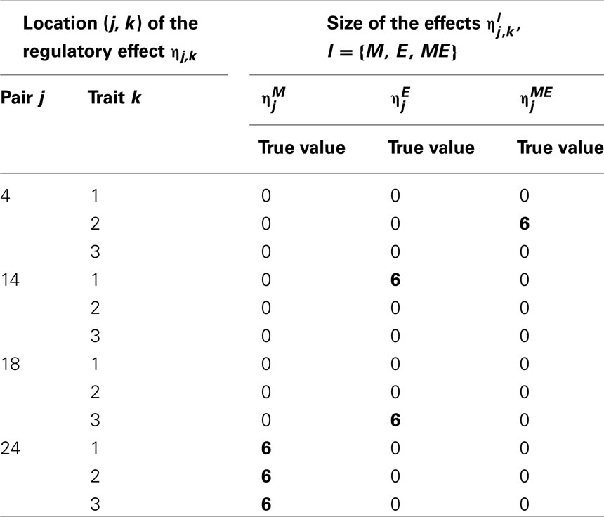
Table 1. Locations of the non-zero effects: for the first trait, there is marker ${\eta }_{24,1}^M$, and expression ${\eta }_{14,1}^E$ components, for the second trait, marker ${\eta }_{24,2}^M,$ and a mixed genotype × expression interaction ${\eta }_{4,2}^{ME},$ and for the third trait, marker ${\eta }_{24,3}^M,$ and expression ${\eta }_{18,3}^E.$

We investigated the model performance in the presence of uncorrelated and correlated cQTL residuals, noting that uncorrelated cQTL residuals do not necessary imply uncorrelated traits since the traits can still be correlated under uncorrelated cQTL residuals owing for instance to pleiotropy. The simulated data with uncorrelated cQTL residual represented our full test set for comparing the multi-trait and single-trait models, whereas the simulated data with correlated cQTL residuals data were merely used to test how well our multi-trait model is able to estimate the cQTL residual covariance structure.

To simulate data with small heritabilities and uncorrelated cQTL residuals, the elements of the residual covariance matrix S were arbitrarily fixed as $S=\left(\begin{array}{ccc}\hfill 139.1\hfill & \hfill \hfill & \hfill \hfill \\ \hfill 0\hfill & \hfill 123.3\hfill & \hfill \hfill \\ \hfill 0\hfill & \hfill 0\hfill & \hfill 128.1\hfill \\ \hfill \hfill \end{array}\right)$, where the elements above the main diagonal have been omitted due to symmetry. On average, the standard deviations ${\widehat{\sigma }}_{Y_k}^{}$ of the simulated cQTL data over the N = 100 individuals for Trait 1, Trait 2, and Trait 3 were 13.62, 12.92, and 12.50, respectively, implying a joint heritability h² ≈ (0.25, 0.26, 0.18)^T, where $h_k^2=\left({\widehat{\sigma }}_{Y_k}^2-{\sigma }_{S_k}^2\right)∕{\widehat{\sigma }}_{Y_k}^2,$ k=1,2,3 and ${\sigma }_{S_k}^2={\mathbf{\text{S}}}_{kk}.$ Although these heritability values are small and may not provide the best conditions for investigating the model behavior, they do reflect the reality of values that are commonly encountered in real-world genetic data.

To simulate data with large heritabilities and correlated cQTL residuals, we set the elements of the residual covariance matrix as $S=\left(\begin{array}{ccc}\hfill 154\hfill & \hfill \hfill & \hfill \hfill \\ \hfill 130\hfill & \hfill 112\hfill & \hfill \hfill \\ \hfill 133\hfill & \hfill 113\hfill & \hfill 117\hfill \\ \hfill \hfill \end{array}\right)$. On average, the standard deviations of the simulated cQTL data over the N = 100 individuals for Traits 1, 2, and 3 were 17.45, 17.92, and 16.75, respectively, implying a joint heritability h² ≈ (0.49, 0.65, 0.58)^T.

Analysis of simulated data

Simulation of missing marker and expression data. Often considerable amount of missing marker and expression data may occur at random positions in the data matrix. Also, due to financial constraints, marker data may be available for much larger group of individuals than expression data. Following Sillanpää and Noykova (2008), we considered the following missing data scenarios for simulating data under uncorrelated cQTL residuals, in order to investigate the sensitivity of the method/model to the amount of randomly missing values: (1) 10% of both marker genotypes G_i,j and gene expressions E_i,j coded as missing. (2) 10% of marker genotypes G_i,j and 30% of gene expressions E_i,j coded as missing. We also investigated a third scenario with 10% of marker genotypes G_i,j and 50% of gene expressions E_i,j coded as missing, but 50% turned out to be a too high and inconclusive amount of missingness. We do not report the results for this case.

Data analyses under the multi-trait and single-trait cQTL models. We analyzed the simulated (uncorrelated cQTL residual) data under missing data scenarios 1 and 2 using two different missing data models namely, the model MD1, shown on Figure 1, where $E_{i,j}\sim N\left(I_j{\mu }_j{A}_j{G}_{i,j},{\sigma }_{0_{}}^2\right)$ for each individual i and marker-gene pair j, and the simpler MD2 model $E_{i,j}\sim N\left(0,{\sigma }_0^2\right),$ where $p\left(E|I,\mu ,A,G,{\sigma }_0^2\right)$ is simply replaced by $p\left(E|{\sigma }_0^2\right)$.

For both the MD1 and MD2 versions of the model, we assumed a Bernoulli prior for indicators $I_{k,j}^l|s^l\sim \text{Bern}\left(s^l\right),$ with two different pre-specified parameter values for s^l namely, (1) s^l = 0.013 = 1/(3 × 25), which implies fewer non-zero indicator elements than the true simulated value, and (2) s^l = 0.09 implying a slightly larger proportion of non-zero effects.

We first analyzed the simulated data using our multi-trait model, with s^l set to 0.013 and 0.09, and subsequently fitted the single-trait cQTL model of Sillanpää and Noykova (2008) to each trait separately, with s^l set to 0.0033, 0.013, and 0.09.

We used MCMC simulation through the Bayesian freeware OpenBUGS 2.2.0 (Thomas et al., 2006) to sample from the joint posterior of the model parameters. The BUGS code is available from the authors upon request. The reported results are based on 100,000 MCMC iterations, the first 10,000 of which were discarded as burn-in. The convergence of the MCMC was assessed through visual inspection of trace plots. The 100,000 MCMC iterations took roughly 256,000 and 59,000 s for the multi-trait and single-trait models, respectively on a PC equipped with an Intel(R) Core(TM)2 Duo CPU T550 at 1.83G Hz and 3.00GB of RAM.

We focus attention on the estimates (posterior means), ${\bar{\eta }}_{j,k}^l,$ of the cQTL effects ${\eta }_{j,k}^l,$ l = {M, E, ME}, j = 1, …, N_p and as a rule of thumb, we consider ${\eta }_{j,k}^l$ to be non-negligible if its posterior mean is equal or larger than 0.2 in absolute value i.e., if $\left|{\bar{\eta }}_{j,k}^l\right|\ge 0.2.$ Thus, all estimated ${\eta }_{j,k}^l$ such that $\left|{\bar{\eta }}_{j,k}^l\right|<0.2$ were set to zero and deemed negligible.

Results

Under uncorrelated cQTL residual data, the multi-trait model broadly outperformed its single-trait counterpart. It is well known that the single-trait approach is prone to poor statistical power in the presence of correlated responses. In what follows, we provide a fairly detailed account of the results concerning the analysis based on simulated data under uncorrelated cQTL residuals, and only succinctly comment on the ability of the multi-trait model to accommodate the covariance structure of cQTL residuals. The reported results are typical of the model performances in different settings.

Tables 2–5 give the true cQTL effects ${\eta }_{j,k}^l$ and their estimated values as posterior means ${\bar{\eta }}_{j,k}^l$ under the two specifications (MD1 and MD2) of the HB multi-trait cQTL model for different missing value scenarios and different values of the prior inclusion probability s^l. In all tables, a bold font is used to indicate the positions where the true or estimated effect was non-zero. The shaded cells indicate false positives or false negatives.

TABLE 2

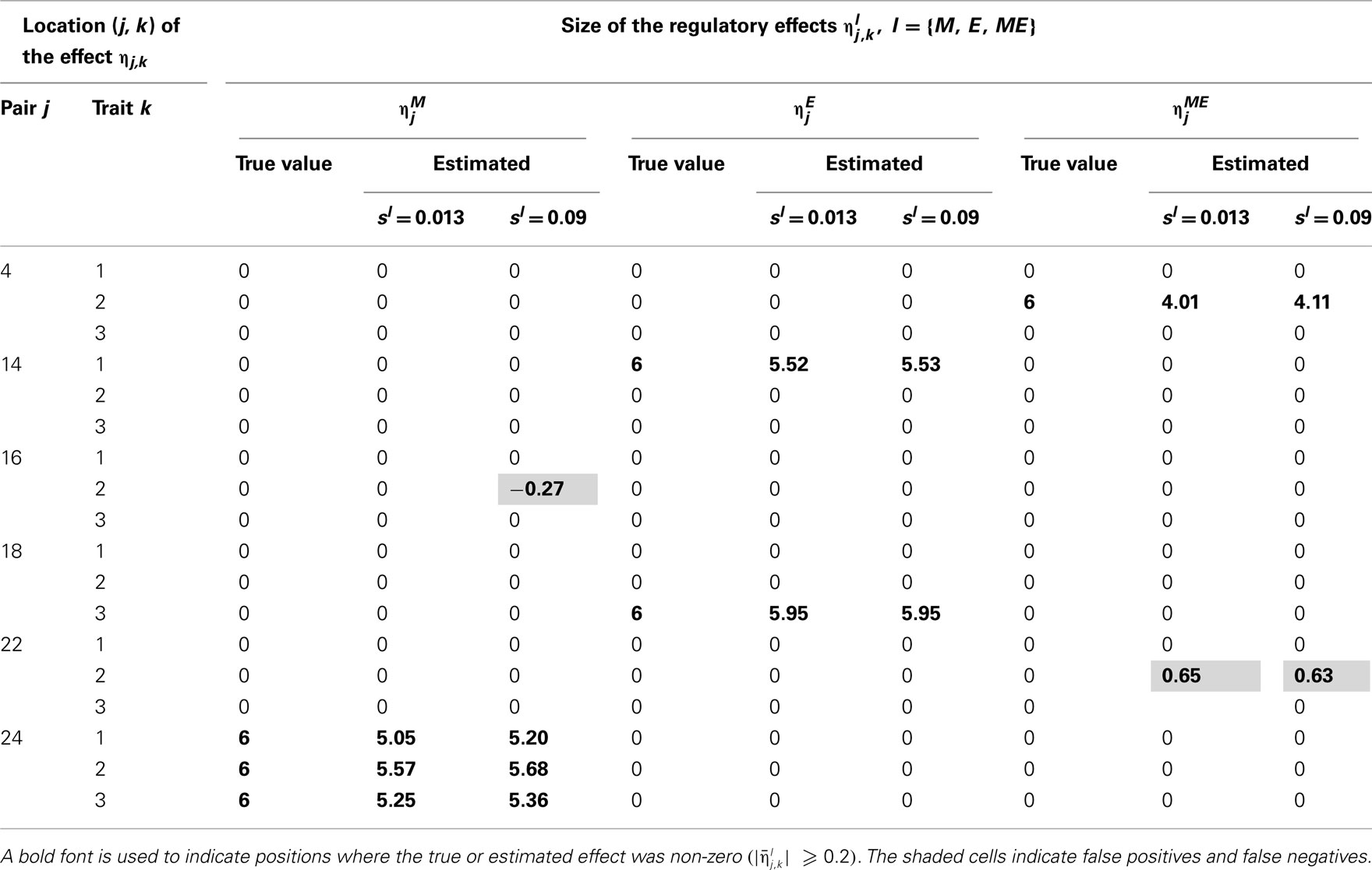
Table 2. True and estimated (posterior means) cQTL effects under the MD1 version of the HB multi-trait cQTL model with 10% markers and 10% expressions coded as missing and different values of Bernoulli parameter s^l.

TABLE 3

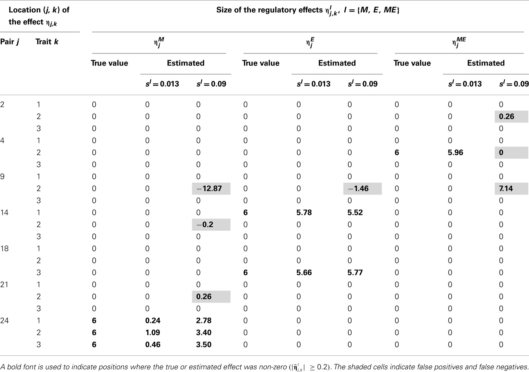
Table 3. True and estimated (posterior means) cQTL effects under the MD1 version of the HB multi-trait cQTL model with 10% markers and 30% expressions coded as missing and different values of Bernoulli parameter s^l.

TABLE 4

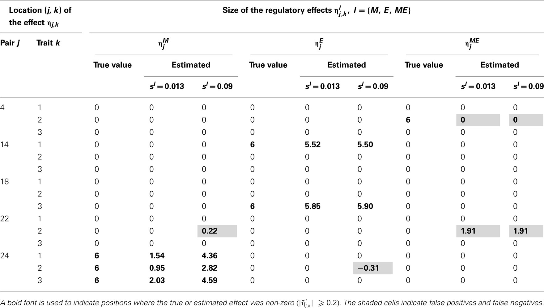
Table 4. True and estimated (posterior means) cQTL effects under the MD2 version of the HB multi-trait cQTL model with 10% markers and 10% expressions coded as missing and different values of Bernoulli parameter s^l.

TABLE 5

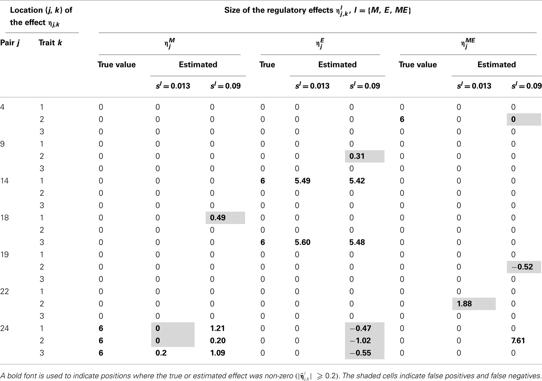
Table 5. True and estimated (posterior means) cQTL effects under the MD2 version of the HB multi-trait cQTL model with 10% markers and 30% expressions coded as missing and different values of Bernoulli parameter s^l.

The results shown in Tables 2–5 suggest that the multi-trait cQTL model is more effective at identifying cQTLs. The better performance was observed when s^l was set to be small (0.013), owing presumably to the fact that a lower s^l value implies a stronger constraint on the presence of effect, which may prevent redundant effects from showing up. Conversely, a higher s^l value increases the model propensity to false discovery, but may result in more accurate estimates since in this case the effect sizes experience relatively less shrinkage. However, the point of cQTL analysis is variable selection rather than estimation, meaning that the accurate estimation of the effects is not essential. It is also clear from our results that the mixed phenotype × expression η^ME effects are the most difficult to identify. Moreover, the FDR proved to increase with the proportion of missing data. Finally, cQTL identification was more effective under the MD1 specification. The model was particularly ineffective at identifying the mixed regression parameter η^ME under the MD2 specification, and was more prone to false discovery than under the MD1 specification. A potential explanation for this propensity to false discovery is the lack of constraint in the missing data model $E_{i,j}\sim N\left(0,{\sigma }_0^2\right)$ under MD2.

More interestingly, the cQTL residual covariance matrix S was estimated to an appreciable degree of accuracy under the multi-trait model in case of correlated cQTL residuals. The estimates (posterior medians) of the components of S under the MD1 specification of the multi-trait model with 10% of markers and 10% expression coded as missing and s^l = 0.013 was $\tilde{S}\approx \left(\begin{array}{ccc}\hfill 122.6\hfill & \hfill \hfill & \hfill \hfill \\ \hfill 96.9\hfill & \hfill 83\hfill & \hfill \hfill \\ \hfill 100.9\hfill & \hfill 80\hfill & \hfill 87.5\hfill \\ \hfill \hfill \end{array}\right)$, which is fairly close to the simulated values.

In single-trait cQTL analyses, the results were comparable across the three traits. Tables 6–9 give the results for single-trait analysis of trait 1 based on simulated data under uncorrelated cQTL residuals. These results are representative of the full set of (uncorrelated data) results from the single-trait cQTL analysis.

TABLE 6

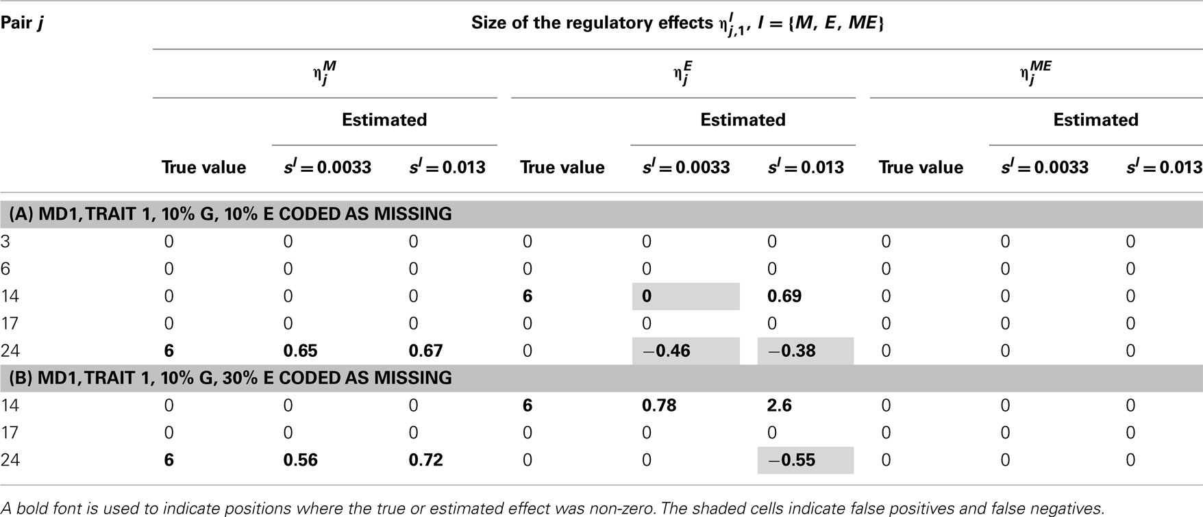
Table 6. True and estimated (posterior means) cQTL effects in the analysis of Trait 1 using the MD1 version of the HB single-trait cQTL model with (A) 10% markers and 10% expressions coded as missing and (B) 10% markers and 30% expressions coded as missing, and different values of Bernoulli parameter s^l.

TABLE 7

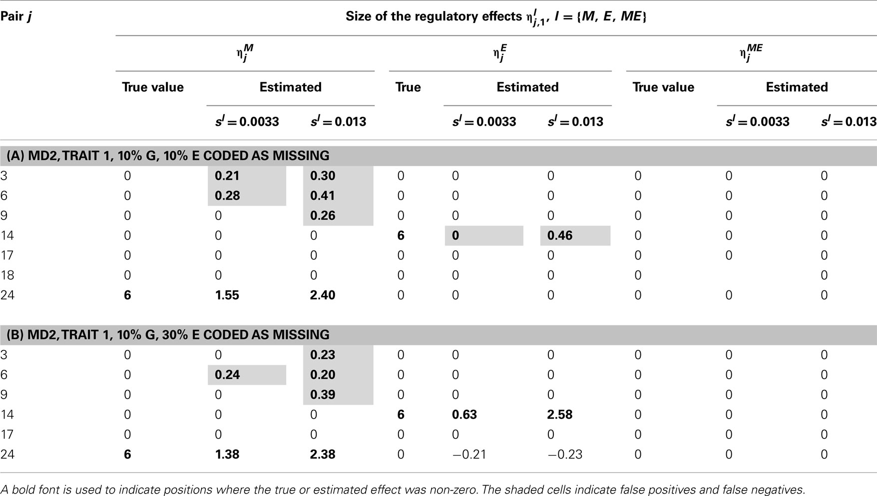
Table 7. True and estimated (posterior means) cQTL effects in the analysis of Trait 1 using the MD2 version of the HB single-trait cQTL model with (A) 10% markers and 10% expressions coded as missing and (B) 10% markers and 10% expressions coded as missing, and different values of s^l.

TABLE 8

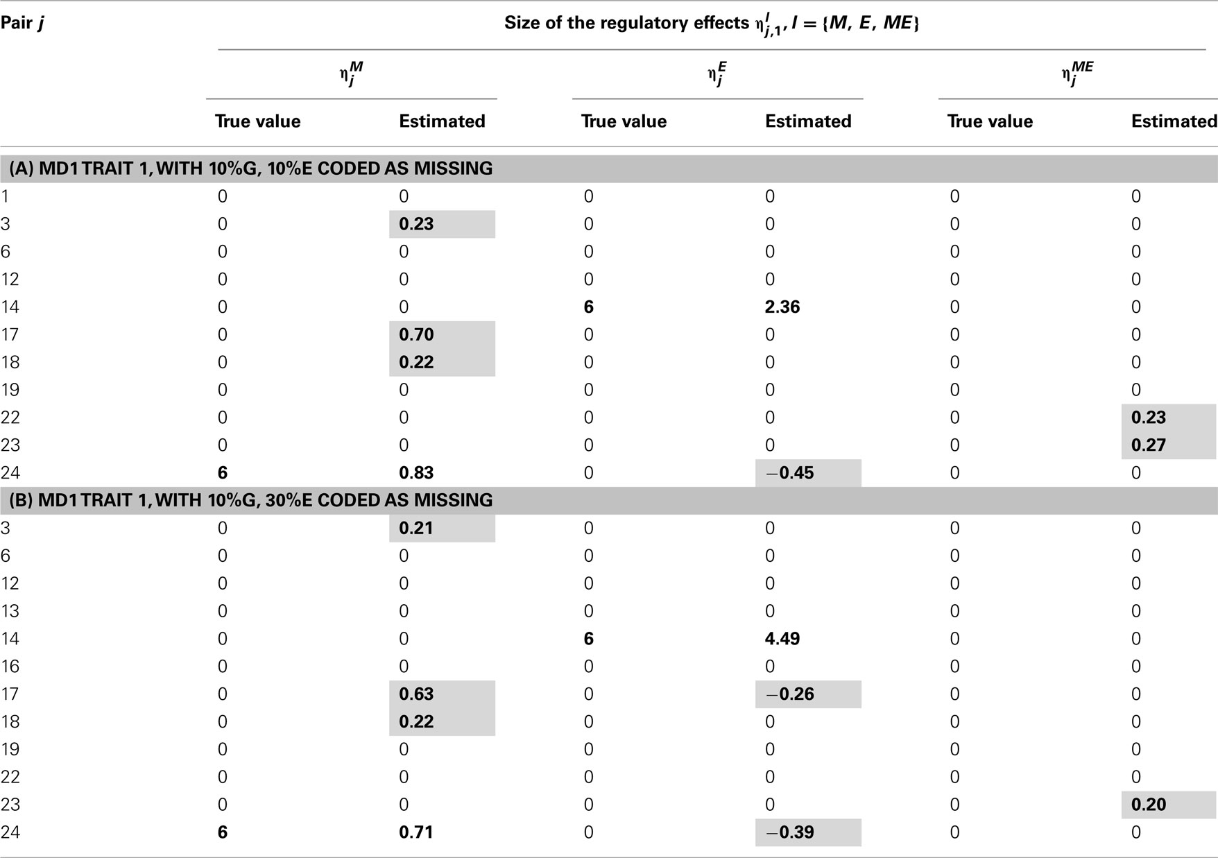
Table 8. True and estimated (posterior means) cQTL effects in the analysis of Trait 1 using the MD1 version of the HB single-trait cQTL model with (A) 10% markers and 10% expressions coded as missing and (B) 10% markers and 30% expressions coded as missing, and for s^l = 0.09.

TABLE 9

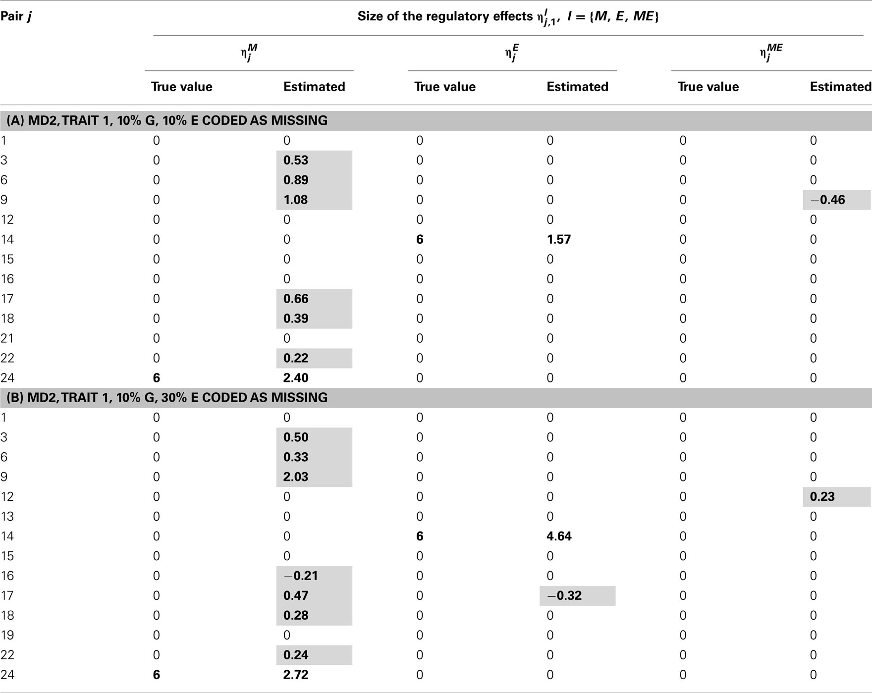
Table 9. True and estimated (posterior means) cQTL effects in the analysis of Trait 1 using the MD2 version of the HB single-trait cQTL model with (A) 10% markers and 10% expressions coded as missing and (B) 10% markers and 30% missing expressions coded as missing, and for Bernoulli parameter s^l = 0.09.

In single-trait cQTL analysis too, the model performed better under the MD1 specification when s^l was low (0.0033 and 0.013). Although the model was capable of detecting roughly all true effects under both the MD1 and MD2 specifications, the FDR was relatively higher under the MD2 specification. The number of false positives appeared to increase with the proportion of missing expressions under both specifications.

Discussion

The conceptual description of the new HB multi-trait cQTL model was presented in this paper and it provides a promising framework for integrating molecular markers and gene transcript levels to dissect the genetic architecture of complex clinical traits. Our results demonstrate that the multi-trait approach enhances the power and should be considered seriously in cQTL mapping framework. Because of its conceptual nature, it is worth emphasizing that practical and scalable implementations of the method are beyond the scope of this paper. Often considerable amount of missing marker and expression data may occur at random positions in the data matrix with higher missing rate for expressions than for marker genotypes. The analyses here were based on two missing data scenarios with either 10% of both marker genotypes G_i,j and gene expressions E_i,j coded as missing, or 10% of marker genotypes G_i,j and 30% of gene expressions E_i,j coded as missing. For both the multi-trait and single-trait approaches, we considered two different model specifications depending on the way the missing expression data were modeled namely, MD1 (shown in Figure 1) where $E_{i,j}\sim N\left(I_j{\mu }_j{A}_j{G}_{i,j},{\sigma }_0^2\right),$ and MD2 where $E_{i,j}\sim N\left(0,{\sigma }_0^2\right).$

Under both MD1 and MD2 specifications, the priors on the inclusion indicators, $I_{k,j}^l|s^l,$ for the cQTL effects were defined as $I_{k,j}^l|s^l\sim \mathit{\text{Bern}}\left(s^l\right),$ and different pre-specified values were used for prior inclusion probability s^l, including s^l = 0.013 = 1/(3 × 25), which assumes fewer non-zero indicator elements (i.e., a sparser model) than the true simulated value 0.08, and the slightly larger value s^l = 0.09.

For the sake of comparison, we also analyzed each trait separately through the single-trait cQTL model with three different values for s^l namely, 0.0033, 0.013, and 0.09. The single-trait analyses were confined to simulated data under uncorrelated cQTL residuals.

The multi-trait model performed better under the MD1 specification in terms of identifying cQTLs for small to moderate (10–30%) proportion of missing expression data, and tended to produce fewer false positives. Under the MD2 specification, the model failed consistently to identify the mixed genotype × expression effects η^ME when s^l was large (0.09), regardless of the amount of missing data, whilst under the same conditions. Overall, the MD1 version of the model was capable of identifying 75% of the mixed genotype × expression effects.

The out-performance of the MD1 version of the model over its MD2 counterpart in terms of the power to identify the non-zero cQTL effects and an overall lower rate of false positives was also observed in single-trait cQTL analyses. This suggests that the handling of missing values can make a difference to the model performance.

The multi-trait HB cQTL model showed over its single-trait counterpart an increased power of identifying cQTLs with a lower rate of false positives. The covariance structure of cQTL residuals was also estimated under the multi-trait model to a fair degree of accuracy. The multi-trait approach to cQTL analysis is valuable for addressing a number of practical challenges arising in the presence of correlated phenotypic traits, as is the case for many complex disease syndromes like asthma (e.g., Kim and Xing, 2009). Moreover, a multi-trait model provides a framework for investigating a number of biologically interesting hypotheses involving multiple traits, such as pleiotropy. In conclusion, the HB approach to multi-trait cQTL analysis holds great promises for elucidating the underlying biology of complex clinical traits.

Conflict of Interest Statement

The authors declare that the research was conducted in the absence of any commercial or financial relationships that could be construed as a potential conflict of interest.

Acknowledgments

We are grateful to two anonymous referees for their constructive comments. This work was supported by a research grant from the Academy of Finland and the University of Helsinki’s research funds.

References

Borevitz, J. O., Liang, D., Plouffe, D., Chang, H. S., Zhu, T., Weigel, D., Berry, C. C., Winzeler, E., and Chory, J. (2003). Large-scale identification of single-feature polymorphisms in complex genomes. Genome Res. 13, 513–523.

Pubmed Abstract | Pubmed Full Text | CrossRef Full Text

Breitling, R., Li, Y., Tesson, B. M., Fu, J., Wu, C., Wiltshire, T., Gerrits, A., Bystrykh, L. V., de Haan, G., Su, A. I., and Jansen, R. C. (2008). Genetical genomics: spotlight on QTL hotspots. PLoS Genet. 4, e1000232. doi:10.1371/journal.pgen.1000232

CrossRef Full Text

Brem, R. B., Yvert, G., Clinton, R., and Kruglyak, L. (2002). Genetic dissection of transcriptional regulation in budding yeast. Science 296, 752–755.

Pubmed Abstract | Pubmed Full Text | CrossRef Full Text

Cheung, V. G., Spielman, R. S., Ewens, K., Weber, T. M., Morley, M., and Burdick, J. T. (2005). Mapping determinants of human gene expression by regional and genome-wide association. Nature 437, 1365–1369.

Pubmed Abstract | Pubmed Full Text | CrossRef Full Text

de Koning, D. J., and Haley, C. S. (2005). Genetical genomics in humans and model organisms. Trends Genet. 21, 377–381.

Pubmed Abstract | Pubmed Full Text | CrossRef Full Text

Drake, T. A., Schadt, E. E., and Lusis, A. J. (2006). Integrating genetic and gene expression data: application to cardiovascular and metabolic trait in mice. Mamm. Genome 17, 466–479.

Pubmed Abstract | Pubmed Full Text | CrossRef Full Text

Gelman, A., Carlin, J. B., Stern, H. S., and Rubin, D. B. (2003). Bayesian Data Analysis, 2nd Edn. New York: Chapman and Hall.

Gilks, W. R., Richardson, S., and Spiegelhalter, D. J. (eds). (1996). Markov Chain Monte Carlo in Practice. London: Chapman and Hall.

Hoti, F., and Sillanpää, M. J. (2006). Bayesian mapping of genotype x expression interactions in quantitative and qualitative traits. Heredity 97, 4–18.

Pubmed Abstract | Pubmed Full Text | CrossRef Full Text

Jansen, R. C., and Nap, J.-P. (2001). Genetical genomics: the added value from segregation. Trend Genet. 17, 388–391.

CrossRef Full Text

Jiang, C., and Zeng, Z.-B. (1995). Multiple trait analysis of genetic mapping for quantitative trait loci. Genetics 140, 1111–1127.

Pubmed Abstract | Pubmed Full Text

Kendziorski, C. M., Chen, M., Yuan, M., Lan, H., and Attie, A. D. (2006). Statistical methods for expression quantitative trait loci (eQTL) mapping. Biometrics 62, 19–27.

Pubmed Abstract | Pubmed Full Text | CrossRef Full Text

Kim, S., and Xing, E. P. (2009). Statistical estimation of correlated genome associations to a quantitative trait network. PLoS Genet. 5, e1000587. doi:10.1371/journal.pgen.1000587

CrossRef Full Text

Lee, E., Cho, S., Kim, K., and Park, T. (2009). An integrated approach to infer causal associations among gene expression, genotype variation, and disease. Genomics 94, 269–277.

Pubmed Abstract | Pubmed Full Text | CrossRef Full Text

Li, H., and Deng, H. (2010). Systems genetics, bioinformatics and eQTL mapping. Genetica 138, 915–924.

Pubmed Abstract | Pubmed Full Text | CrossRef Full Text

Liu, B., de la Fuente, A., and Hoeschele, I. (2008). Gene network inference via structural equation modeling in genetical genomics experiments. Genetics 178, 1763–1776.

Pubmed Abstract | Pubmed Full Text | CrossRef Full Text

Liu, J., Liu, Y., Liu, X., and Deng, H.-W. (2007). Bayesian mapping of QTL for multiple complex traits with the use of variance components. Am. J. Hum. Genet. 81, 304–320.

Pubmed Abstract | Pubmed Full Text | CrossRef Full Text

Mackay, T. F. C. (2009). Q&A: genetic analysis of quantitative traits. J. Biol. 8, 23.

Pubmed Abstract | Pubmed Full Text | CrossRef Full Text

Mutshinda, C. M., O’Hara, R. B., and Woiwod, I. P. (2008). Species abundance dynamics under neutral assumptions: a Bayesian approach to the controversy. Funct. Ecol. 22, 340–347.

CrossRef Full Text

Mutshinda, C. M., and Sillanpää, M. J. (2010). Extended Bayesian LASSO for multiple quantitative trait loci mapping and unobserved phenotype prediction. Genetics 186, 1067–1075.

Pubmed Abstract | Pubmed Full Text | CrossRef Full Text

Mutshinda, C. M., and Sillanpää, M. J. (2011). Bayesian shrinkage analysis of QTLs under shape-adaptive shrinkage priors, and accurate re-estimation of genetic effects. Heredity 107, 405–412.

Pubmed Abstract | Pubmed Full Text | CrossRef Full Text

Pikkuhookana, P., and Sillanpää, M. J. (2009). Correcting for relatedness in Bayesian models for genomic data association analysis. Heredity 103, 223–237.

Pubmed Abstract | Pubmed Full Text | CrossRef Full Text

Ronald, J., Akey, J. M., Whittle, J., Smith, E. N., Yvert, G., and Kruglyak, L. (2005). Simultaneous genotyping, gene-expression measurement, and detection of allele-specific expression with oligonucleotide arrays. Genome Res. 15, 284–291.

Pubmed Abstract | Pubmed Full Text | CrossRef Full Text

Schadt, E. E., Lamb, J., Yang, X., Zhu, J., Edwards, S., Guhathakurta, D., Sieberts, S. K., Monks, S. A., Reitman, M., Zhang, C., Lum, P. Y., Leonardson, A., Thieringer, R., Metzger, J. M., Yang, L., Castle, J., Zhu, H., Kash, S. F., Drake, T. A., Sachs, A., and Lusis, A. J. (2005). An integrative genomics approach to infer causal associations between gene expression and disease. Nat. Genet. 37, 710–717.

Pubmed Abstract | Pubmed Full Text | CrossRef Full Text

Schadt, E. E., Monks, S. A., and Friend, S. H. (2003). A new paradigm for drug discovery: integrating clinical, genetic, genomic and molecular phenotype data to identify drug targets. Biochem. Soc. Trans. 31, 437–443.

Pubmed Abstract | Pubmed Full Text | CrossRef Full Text

Sillanpää, M. J., and Noykova, N. (2008). Hierarchical modeling of clinical and expression quantitative trait loci. Heredity 101, 271–284.

Pubmed Abstract | Pubmed Full Text | CrossRef Full Text

Thomas, A., O’Hara, R. B., Ligges, U., and Sturtz, S. (2006). Making BUGS open. R News 6, 17–21.

Wittkopp, P. J. (2005). Genomic sources of regulatory variation in cis and in trans. Cell. Mol. Life Sci. 62, 1779–1783.

Pubmed Abstract | Pubmed Full Text | CrossRef Full Text

Wu, C., Delano, D. L., Mitro, N., Su, S. V., Janes, J., McClurg, P., Batalov, S., Welch, G. L., Zhang, J., Orth, A. P., Walker, J. R., Glynne, R. J., Cooke, M. P., Takahashi, J. S., Shimomura, K., Kohsaka, A., Bass, J., Saez, E., Wiltshire, T., and Su, A. I. (2008). Gene set enrichment in eQTL data identifies novel annotations and pathway regulators. PLoS Genet. 4, e1000070. doi:10.1371/journal.pgen.1000070

CrossRef Full Text

Xu, S. (2003). Estimating polygenic effects using markers of the entire genome. Genetics 163, 789–801.

Pubmed Abstract | Pubmed Full Text

Zou, W., Aylor, D. L., and Zeng, Z.-B. (2007). eQTL Viewer: visualizing how sequence variation affects genome-wide transcription. BMC Bioinformatics 8, 7. doi:10.1186/1471-2105-8-7

CrossRef Full Text