Large Homogeneous Genome Regions (Isochores) in Soybean [Glycine Max (L.) Merr.]

The landscape of plant genomes, while slowly being characterized and defined, is still composed primarily of regions of undefined function. Many eukaryotic genomes contain isochore regions, mosaics of homogeneous GC content that can abruptly change from one neighboring isochore to the next. Isochores are broken into families that are characterized by their GC levels. We identified 4,339 compositionally distinct domains and 331 of these were identified as long homogeneous genome regions (LHGRs). We assigned these to four families based on finite mixture models of GC content. We then characterized each family with respect to exon length, gene content, and transposable elements. The LHGR pattern of soybeans is unique in that while the majority of the genes within LHGRs are found within a single LHGR family with a narrow GC range (Family B), that family is not the highest in GC content as seen in vertebrates and invertebrates. Instead Family B has a mean GC content of 35%. The range of GC content for all LHGRs is 16–59% GC which is a larger range than what is typical of vertebrates. This is the first study in which LHGRs have been identified in soybeans and the functions of the genes within the LHGRs have been analyzed.

Introduction

The genomes of living organisms are often organized into unique patterns, the purposes of which are mostly unknown. It has been reported that at least some eukaryotic genomes contain isochore regions, mosaics of homogeneous GC content that abruptly change from one neighboring isochore to the next. In vertebrates, isochore regions have been defined as segments of DNA, typically above 300 kb, that are homogeneous (AT- or GC-rich) with sharp boundaries from the neighboring stretches of DNA (Constantini et al., 2009).

Isochores were first observed using ultracentrifugation in CsCl density gradients (Macaya et al., 1976). DNA fractionation by ultracentrifugation, cytogenetic analyses, and recently, analyses of genes and genome sequences, has been utilized to identify these regions. With advances in technology and the availability of whole genome sequences isochores can now be identified with more precision using computational tools. Initially, sliding-window-based methods were used but these techniques can only determine isochores based on the window size used. Surprisingly, fundamental biological properties have been found to be associated with certain isochore families. Repeat sequence distribution, gene density, replication timing, CpG distribution, genic size, and transcript abundance are several of the main features found to associate with isochores (Bernardi, 2004). In vertebrates, these regions have been mapped and named long homogeneous genome regions (LHGRs; Zhang et al., 2010). Recently, LHGRs also have been identified in invertebrates (Cammarano et al., 2009). LHGR GC content is strongly conserved among invertebrate species (Cammarano et al., 2009) as well as among vertebrate species (Constantini et al., 2009). However, vertebrates and invertebrates differ in the GC content of their LHGR families. The existence of LHGRs across two kingdoms suggests that all metazoan genomes may contain LHGRs and suggests a biological or evolutionary importance, yet their function remains unknown.

Long homogeneous genome regions are classified into a number of families based on the frequency distributions of LHGRs across GC percentage (Macaya et al., 1976). Often, members of LHGR families will share similar additional biological features such as frequency of transposable elements (Bernardi, 2004). Multiple peaks in the distribution of content are evident in most species although the demarcation between one LHGR family and the adjacent families have been based on ad hoc decisions. For example, the mid-point between two peaks has been arbitrarily considered a threshold, where one family ends and the next family begins. A different technique was applied in Arabidopsis (Zhang and Zhang, 2004) where the LHGRs were identified as GC-rich (GC content of the LHGR was above the average GC content for the chromosome in which it resided) and AT-rich (GC content of the LHGR was below the average GC content for the chromosome in which it resided) because no distinct peaks within the distribution were observed.

Plants are unique in their wide range of genome size and composition. In the grasses, chromosome size, genome size, and GC content have been found to be evolutionarily associated. Small genomes in the genus Festuca appear to be AT-rich, are better at adapting to extreme environmental conditions, are more species-rich and are rapidly diverging (Smarda et al., 2008). Isochores of plants were initially characterized by looking only at limited stretches of DNA (Salinas et al., 1988; Matassi et al., 1989; Montero et al., 1990). It was determined that the compositional pattern of isochores was different between monocots and dicots (Salinas et al., 1988). Curiously, compositional similarities were found between monocots and warm-blooded vertebrates. Both groups have higher GC content relative to dicots and cold-blooded vertebrates and even higher GC content in coding regions. Warm-blooded vertebrates and monocots also show a similar distribution of housekeeping genes compared to tissue-specific genes with the housekeeping genes having a much higher GC content (Salinas et al., 1988). In a subsequent study, a rapid increase in the GC content of rice was shown and this corresponded with a rapid change in the codon usage patterns of those genes (Wang and Hickey, 2007). In this study they also analyzed the synonymous and non-synonymous differences and determined that the primary difference in GC content is through synonymous differences. While many of these studies have focused on the rapid increase in GC content in the genic regions in monocot plants, several studies have shown that there is a bias in the non-coding regions as well (Wong et al., 2002).

Despite the potential impact that studies of isochores could have on understanding genome evolution, Arabidopsis thaliana is the only plant, until now, in which isochores have been identified and characterized at a whole genome level. In the study of the Arabidopsis genome Zhang and Zhang (2004) identified GC-rich, AT-rich, and centromeric isochores. The centromeric isochores are GC-rich yet a low gene density and different T-DNA insertion sites than the GC-rich isochores without centromeres. Because centromeric regions were contained within a centromeric-isochore, all of the predicted centromere sequences were part of an isochore region (Zhang and Zhang, 2004).

The soybean genome is paleopolyploid with 2n = 40 (Pfeil et al., 2005). Recently it was discovered that 57% of the genome is comprised of repeat-rich heterochromatin. However, in these regions, located near the centromeres, 21.6% of the high-confidence genes were discovered (Schmutz et al., 2010). This genetic compositional makeup and the soybean’s genome size more closely resemble that of human than that of another dicot, A. thaliana. Understanding the role of genome size and compositional pattern could help uncover some of the basic “rules” of genome structure and function during evolution.

Using the recently published genome sequence (Schmutz et al., 2010) we sought an understanding of the LHGRs in the soybean genome. Our goals were to identify the compositionally distinct domains in the genome, isolate the homogenous regions, and classify the families of LHGRs found in the soybean genome. We used the program GC-Profile¹ (Gao and Zhang, 2006; Zhang et al., 2010) to identify compositionally distinct segments within the genome based on nucleotide organization. GC-Profile utilizes a segmentation algorithm and provides a windowless view of the chromosomes. These domains were then given a homogeneity score using the homogeneity index “h” (Zhang and Zhang, 2004). LHGRs were identified based on their homogeneity and was assigned to families using a parametric approach to identify the most likely mixture of distributions (McLachlan and Peel, 2000) underlying the overall distribution of GC content.

Results

LHGRs in the Soybean Genome

We used a segmentation algorithm based on z^′ curves to identify soybean LHGRs. The z^′ curve separates the entire chromosome into non-overlapping, compositionally distinct domains based on the nucleotide sequence. There is an inverse relationship between GC content and the z^′ curve. Thus, when the slope of the curve is positive it is indicative of a decreasing GC content. The soybean genome is composed of many compositionally segmented regions similar to what has been observed in pig (Zhang et al., 2010). With the z^′ curve we were able to determine to base-pair resolution the locations of the non-overlapping regions.

To determine whether a region was a LHGR (significantly homogeneous in the GC content), we analyzed each of the domains using an h value (Zhang and Zhang, 2004). The h value evaluates the homogeneity by dividing the variance in the GC content of the region by the variance in the GC content of the whole chromosome. An h value <1 is generally considered to be a region with little variation. We found a total of 4,339 compositionally distinct domains in the 20 chromosomes of the soybean genome. The h values of our regions ranged from 0.0001 to 4.17. We decided to define our LHGRs as regions with an h value less than 0.01. Using this criterion, 331 LHGRs were identified (Table S1 in Supplementary Material).

LHGR Families

The distribution of the 331 LHGRs appeared to be a mixture of at least four overlapping distributions of GC content (Figure 1).

FIGURE 1

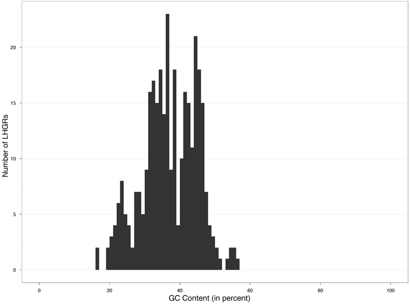
Figure 1. Distribution of LHGRs (binned into 1% GC intervals) across GC content (in percent).

To determine the most number of components within this mixture of distributions we used a parametric approach in which we modeled the distribution as:

$f\left(y;\text{Ψ}\right)={\sum }_{i=1}^g{\text{Π}}_i\text{ϕ}\left(y_i;{\upsilon }_i,{\sigma }_i\right);$

where i represents the number of mixtures, or groups, π_℩ are unknown, but estimable mixing proportions and

$\varphi \left(y_i;{\upsilon }_i,\sigma \right)=\left\{{\left(2\pi \right)}^{-1∕2}{\sigma }_i^{-1}\right\}exp\left\{-1∕2{\left(y_i-{\upsilon }_i\right)}^2∕{\sigma }_i^2\right\}$

with unknown, but estimable means and variances. We calculated the –log(likelihood) for each model beginning with g = 1 and proceeded to sequentially add groups until no significant improvement of the –log(likelihood) was observed (Table 1).

TABLE 1

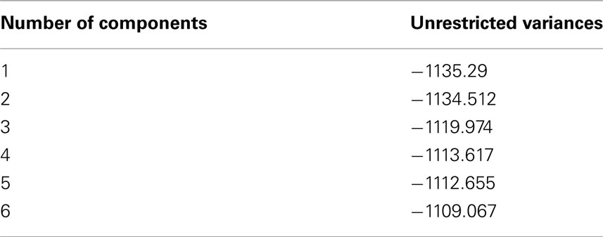
Table 1. Value of the log of the likelihood for the mixture components.

We found that four groups produced the best fit to the data. Based on this analysis the estimated average GC content was 24, 35, 44, and 55% (Figure 2) with 41, 152, 123, and six members in each family, respectively. This translated into family-weighted values of 0.13, 0.49, 0.36, and 0.02, respectively. This analysis permitted us to determine how much each of our distributions overlapped, i.e., how much of one family overlapped into another family’s distribution. The amount of Family A (24%) in Family B (35%) was 10%, the amount of B in A was 2.6%. The estimated amount of B in C (45%) was 6% while the amount of C in B was 5%. The amount of C in D (55%) was 0.01% while the amount of D in C was 1%. With this information we can recognize the amount of bias, for example, that Family C puts on Family B (5%) when looking at the biological properties. This would mean that for each of the LHGRs we classified as a member of Family B LHGR, there is a five percent chance that the LHGR is actually from Family C.

FIGURE 2

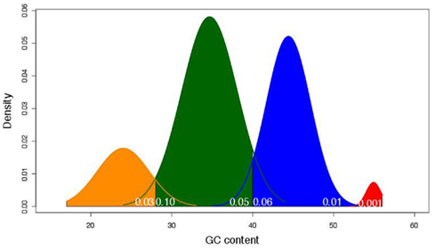
Figure 2. The mixture model of frequency distributions of the four LHGR families across GC content (in percentage). The different colors represent the different families. Yellow is Family A, green is Family B, blue is Family C, and red is Family D. The numbers in white at the base of the density distributions represent the amount of the overlap estimated to come from the adjacent family. For example, the 0.03 value at the base of Family A (yellow) indicates the amount of that family’s distribution that may be attributed to Family B (green).

LHGR Size and Location

Table 2 shows the distribution of LHGRs across chromosomes and the respective chromosome length. The number of LHGRs per chromosome does not appear to be associated with the size of the chromosome. For example, chromosomes 3, 4, 7, 9, 13, and 20 have the largest number of LHGRs (34–45) while two chromosomes (5 and 11) have no LHGRs. The largest LHGR in the soybean genome is 2 mb in length and is located on chromosome 7. There are only three LHGRs that are longer than 1 mb and two of these are located on chromosome 13 (Figure 3). All of the three longest LHGRs are located in the euchromatic arms of the chromosomes and two of them are located near the telomeric region. Although the top ten largest LHGRs are all part of Family B, on average, LHGRs in Family C are the largest which means that a large number of few small LHGRs in Family B. The average size of LHGRs in Family C is 41.1 kb while Family A has an average of 12.8 kb, Family B has an average of 13.8 kb, and Family D has an average of 7.3 kb (Figure 3). This is consistent with results observed in A. thaliana in which the GC-LHGRs are larger than AT-LHGRs and is different than mammals such as pig and human where the AT-LHGRs are larger (Zhang et al., 2010). The average size of the soybean LHGRs is 0.82 mb; smaller than the average size for pigs (0.91 mb) and humans (1.20 mb; Zhang et al., 2010).

TABLE 2

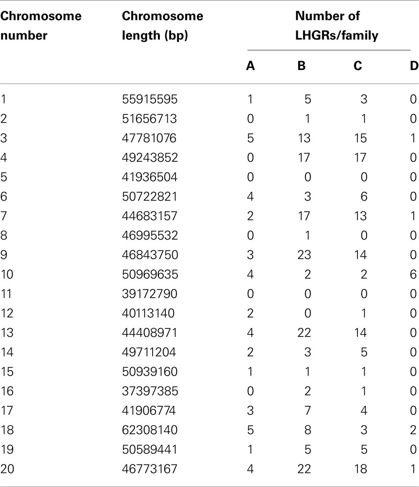
Table 2. The number of LHGRs in each of the 20 soybean chromosomes and the length of the corresponding chromosome.

FIGURE 3

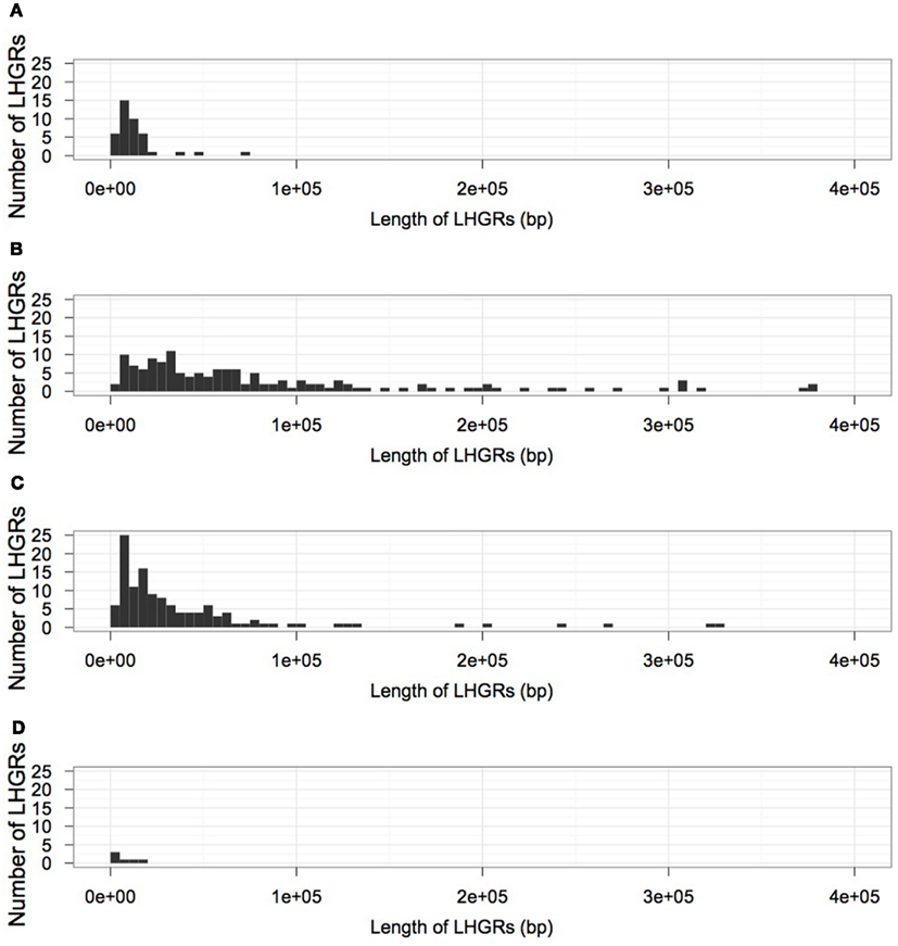
Figure 3. The size distribution of LHGRs in each family; (A) Family A, (B) Family B, (C) Family C, (D) Family D.

Gene Distribution and Transposable Elements in Soybean LHGRs

The majority of the genes located within soybean LHGRs are found in Family B (Table 3). The coding regions of genes in Family C were much larger than those in Family A and Family B (Table 4). This includes the individual exon lengths, the total exon length and the average exon length as well as the total number of exons. As seen in Table 4, the average total exon length for Family C is approximately twice the average total exon length for either Family A or Family B. Interestingly, the average length of the intergenic region, or regions between genes, is 50,000 bp for Family A and 70,000 bp for Family B, and then jumps up to 120,000 bp for Family C showing that not only are the coding regions longer but the non-coding region are also. This is emphasized when you consider that the total intron length and average intron length of genes are the longest for Family C. Family D has been excluded from this comparison as there is only one gene in the LHGRs of Family D.

TABLE 3

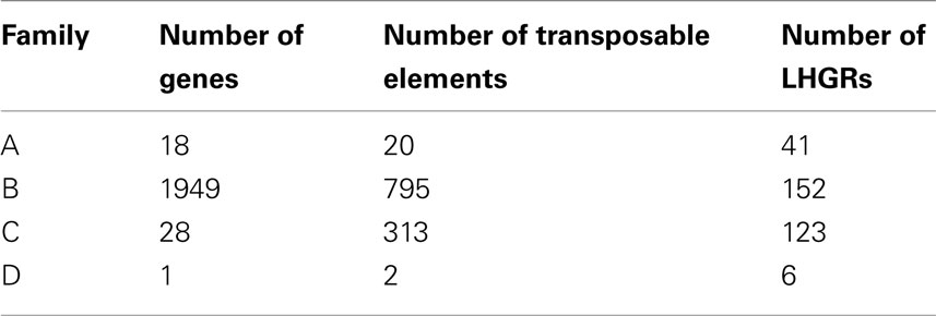
Table 3. The number of genes, number of LHGRs and the number of transposable elements located in each family.

TABLE 4

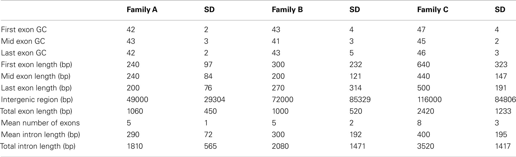
Table 4. The physical parameters of the genes in soybean LHGR Family A, Family B, and Family C.

The number of transposable elements in the LHGRs follows a trend similar to that of gene density. There are more than 2.5× the number of transposable elements in Family B than any of the other families. However, the difference in the density of transposable elements is not as extreme as the difference in gene density per LHGR. The number of genes per LHGR for Family B averages 13 while it is only 0.23 for Family C, which means Family B has about 50 times more genes than Family C. Alternatively, the number of transposable elements per LHGR averages 5 for Family B and 2.5 for Family C.

The transposable elements in the soybean genome are classified as four main families; long interspersed repetitive elements (LINE), long terminal repeat (LTR), helitrons, and (LTRs, LINEs, TIRs, and helitrons; Table 5). The LTR transposable elements are found in the largest abundance across the LHGRs. In each of the families, this is most represented transposable element and in Family D the only transposable elements found were two LTRs. The average length that the transposable element covers the LHGR is largest in Family C and Family D suggesting there are more transposable elements in these LHGRs. There are no LINE transposable elements in Family A, Family C, or Family D and only four were found in Family B. However, it is important to note that there are only 182 identified LINE elements across the soybean genome (Du et al., 2010). Helitrons are also only found in Family A and Family B but also at a very low level (one in Family A, two in Family B).

TABLE 5

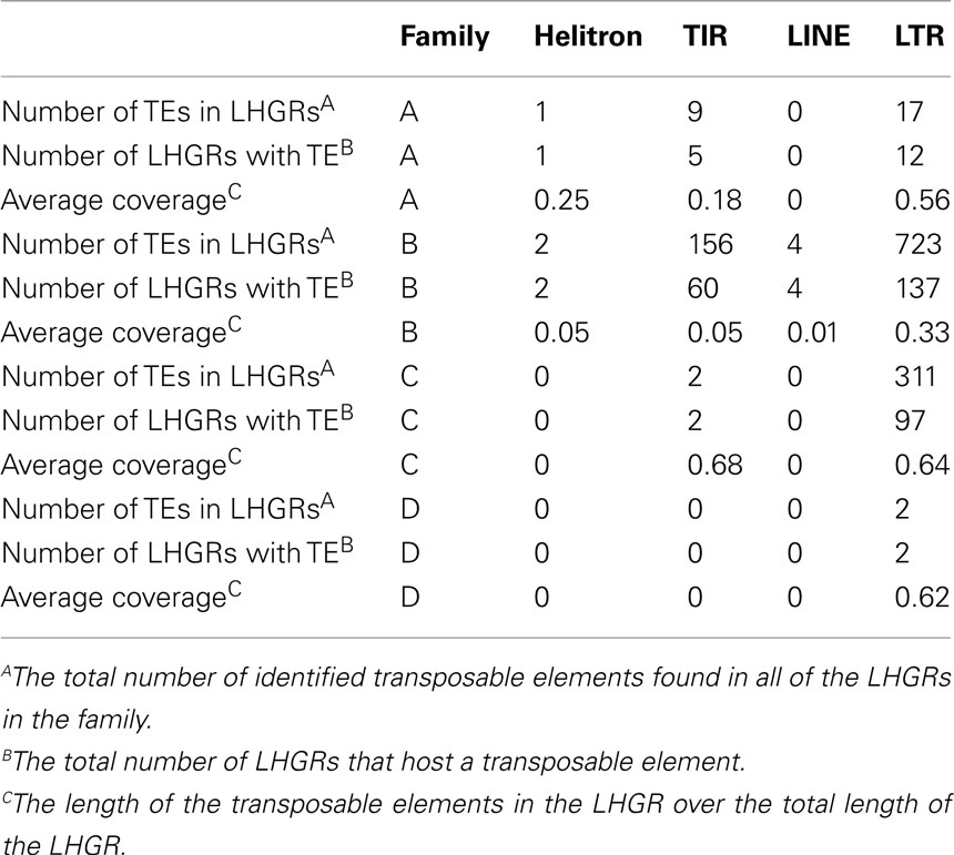
Table 5. The distribution of transposable elements across LHGRs.

Gene Function

To explore the predicted function of the genes in the families we used GO, KEGG, and Panther annotations. Following the protocols of O’Rourke et al. (2009) and Bernardini et al. (2004) we used a Fisher’s exact test (Fisher, 1949) and a Bonferroni correction (Bonferroni, 1936) on Family B to determine which gene functions are over- or under-represented in our gene list compared to those gene functions in the whole soybean genome. Only Family B contained enough genes to use this statistic. Family B contains two groups of genes with GO molecular functions that are over-represented, GO:0008683, 2-oxoglutarate decarboxylase, and GO:0030976, thiamin pyrophosphate binding. The only gene in Family D is Glyma18g06990 and is predicted to be an ATP-dependent CLP protease. The protein products of these genes are involved in cell regulation and they help to stabilize key metabolic enzymes and also remove damaged polypeptides (Clarke, 1999). Next we pooled all of the genes found in the LHGRs and again performed a Fisher’s exact test (Fisher, 1949) with a Bonferroni correction (Bonferroni, 1936). The same two GO molecular functions were over-represented, oxoglutarate decarboxylase and thiamin pyrophosphate binding. This is not surprising as numerous gene functions are shared between the four families.

Interestingly many of the LHGRs are clustered along the genome. Figure 4 shows the physical locations of the LHGRs across the 20 soybean chromosomes separated by family. Surprisingly, many of the LHGRs from different families cluster together along the chromosome.

FIGURE 4

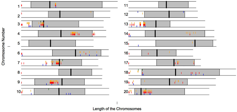
Figure 4. Physical location of LHGRs across chromosomes. The shaded area represents the pericentromeric region (SoyBase). The vertical line represents the predicted centromeric region (SoyBase). Blue bar, Family A; Red bar, Family B; Orange bar, Family C; Green bar, Family D.

Discussion

The definition of an LHGR, or isochore, is based on the homogeneity of the GC content but the transition between homogeneous to heterogeneous is unclear. There are no regions of the genome that are completely homogeneous in the GC content and the question is, at what point does a region shift from being homogeneous to heterogeneous. For this reason we chose a conservative cutoff in hopes of eliminating false positives. Heterogeneous regions could have a separate set of biological properties so understanding the differences between the regions could help differentiate between homogeneous and heterogeneous regions. Therefore, one problem in analyzing isochores is the somewhat arbitrary level of acceptable heterogeneity (Chen and Gao, 2005).

The regions that fit our criteria as homogeneous displayed four overlapping mixture models across the GC percent. We fit our families of LHGR count across GC percent with maximum likelihood. Using this statistic allowed for unrestricted variances as our components appear as an asymmetric multimodal density and there was no evidence to restrict the variance. It was apparent that after four components the log of the likelihood did not significantly change. Using a method to statistically determine the number of components, or families, may be considered in future work however there are many considerations when choosing the statistics. We considered using the LRTS, −2 log λ, which adds a penalty for each additional parameter however there is a problem with the parameters being bounded correctly when used on mixture models as discussed in McLachlan and Peel (2000). In this analysis we used a one parameter, the dimension of GC content. Including other parameters such as biological properties could be useful in future research.

Long homogeneous genome regions have been considered a “fundamental level of genome organization” (Eyre-Walker and Hurst, 2001) and have given us insight into the complexity of large regions of the genome. Various important biological properties such as gene expression, gene size, and transposable element density have been correlated with LHGRs (Aota and Ikemura, 1986; Mouchiroud et al., 1991; Zoubak et al., 1996; Jabbari and Bernardi, 1998). To identify LHGR families in soybean we used a novel approach. Instead of defining our families based on the peak in a graph of GC content by frequency, we used an approach to determine the most likely number of distributions in our data and with that, determined the parameters of each of the families. LHGRs in soybeans comprise four families, each of a different size. There are two predominant families, Family B (35% mean GC) and Family C (44% mean GC) and two minor families, Family A (24% mean GC) and Family D (55% mean GC). This is different from what was found in Arabidopsis where no distinct peaks or families were apparent (Zhang and Zhang, 2004). Soybean exhibits a very wide range of GC content in LHGRs, the lowest LHGR has a 16% GC content and the highest LHGR has a 59% GC content, greater than that found in vertebrates or invertebrates. Vertebrate LHGR families are conserved and are identified as L1 (>37% GC), L2 (37–41% GC), H1 (41–46% GC), H2 (46–53% GC), H3 (>53% GC; Zhang et al., 2010). Peaks, or centers of families, in LHGRs appear approximately in 5% bins while in soybean they appear in approximately 10% bins. The biological or evolutionary significance of this remains unknown.

In previous studies of other genera, a majority of the genes identified resided in one narrow GC range, similar to our observation. However, in most species the gene density increased as the GC content increased (Constantini et al., 2006, 2009; Cammarano et al., 2009), but in soybeans the gene density is highest in the family with the second lowest GC content, Family B (35%). This is similar to what was found in Zebrafish (Constantini et al., 2007a,b). Family B also contains most of the transposable elements. As observed in other species, transposable elements also seem to be enriched in LHGRs at one specific level of GC content and depleted in others (Mouchiroud et al., 1991).

The physical properties of the genes in Family B are similar to those found in Family A and are similar to the average size for a soybean gene. However, the genes in Family C are much larger both in the coding and the non-coding regions than the other two families. Family D has the greatest GC content but only contains one gene. However, it is important to note that Family D consists of only six LHGRs. In previous studies change in gene density correlated with a change in the physical properties of the gene as did the expression level of the gene (Aota and Ikemura, 1986; Zoubak et al., 1996; Woody et al., 2011). It is interesting to note then, that the LHGR families are also correlated with several of these features.

Of all the known genomic properties in plant genomes, transposable elements cover the largest proportion of genomes. Annotating transposable elements at a whole genome level is a very complex task but a whole genome computational analysis was done to identify the transposable elements in the soybean genome (Du et al., 2010). The availability of this database has allowed us to understand the influence transposable elements have on the makeup of LHGRs. The transposable elements in soybean are broken into four main families. Two of the families are in Class 1 (LINEs and LTRs), retrotransposons, and two of the families are in Class II (TIRs and Helitrons), DNA transposons (SoyBase). Repetitive elements make up an estimated 59% of the soybean genome (Schmutz et al., 2010) and this could influence the identification and makeup of LHGRs in soybean. In previous studies, certain families of transposable elements were preferentially located in specific families. For example, in humans Alu retrotransposon density is much higher in GC-rich LHGRs (Hackenberg et al., 2005). In LHGRs, helitrons were only found in the AT-rich LHGRs, Family A, and Family B. Only two helitrons were found in Family B and one in Family A. LTRs are the most abundant transposable element family found in soybean LHGRs. LTRs are also the most abundant transposable elements found in the soybean genome making up about 42% of the genome (Schmutz et al., 2010). The largest quantity of transposable elements are found in Family B and the coverage of is much higher as well. Transposable element coverage increases with an increase in GC content and gene size. Future analysis will need to be done to understand the complex regulatory interactions between these genomic properties.

This is the first study done in plants in which a functional analysis has been conducted on the genes in LHGRs. We analyzed the genes in Family B using a Fisher’s exact test with a Bonferroni correction, to identify which GO functions were under/over-represented. We found that 2-oxoglutarate decarboxylase and thiamin pyrophosphate binding are overrepresented. The two enzymes work closely together as thiamin pyrophosphate is needed to maximize the efficiency of 2-oxoglutarate (Shigeoka and Nakano, 1991) and both are involved in the Krebs cycle (Mitsuda et al., 1975). The similarity in gene function across families is striking. We were unable to perform a statistical analysis on Family A, C, or D independently as there were not enough genes but the function of the genes in these families are consistent with the results found in Family B. However, we were able to pool all of the genes in our analysis into one large group and performed the same statistical analysis. Again we found that 2-oxoglutarate decarboxylase and thiamin pyrophosphate binding are significantly overrepresented which is not surprising as the families share many gene functions. The majority, if not all of the genes in the LHGRs are related to metabolic and cell cycle functions such as ATP and AMP proteases and serine-threonine kinases. In Family D, there is only one gene and even this gene has a metabolic function, ATP-dependent CLP protease. In Arabidopsis, one LHGR and one LHGR-like regions are nucleolar organizer regions while another LHGR is a mitochondrial insertion (Chen and Gao, 2005).

In conclusion, LHGRs (isochores) are identifiable in soybean. LHGRs in soybean share similarity with animals in that gene density is focused in a narrow GC range. The average sizes exhibited by LHGR families resemble the trends found in human and pig. However, plants are unique and possibly quite variable. The GC mean of the four families in soybean is more diverse and thus the families are spread further along the range of GC content than what has been found in animals. Alternatively, the mean of the two groups found in Arabidopsis is much smaller than that found in animals. A comparative analysis of LHGRs in plants could help increase our knowledge of compositional evolution across species and the relationship between evolutionary adaptation and large, conserved blocks of the genomes.

Materials and Methods

Identification of LHGRs

The genome sequence was downloaded from SoyBase (accessed on 02.02.2011). To identify compositionally distinct domains we used a program GC-profile (see text footnote 1; Gao and Zhang, 2006). GC-Profile utilizes a segmentation algorithm that allows for a windowless view of the chromosomes. Each chromosome is considered individually and separated into non-overlapping domains. We used the parameters as suggested in Zhang et al. (2010) with a minimum size of 3 kb and we ignored gaps shorter than 1% of the chromosome. GC-profile is based off of a Z curve which is a way of viewing the unique compositional pattern of each chromosome. The z^′ score is calculated based off of the cumulative A, C, G, and T occurrence along the specific regions.

The homogeneity within the compositionally distinct domains was measured using a homogeneity index h as described in Zhang and Zhang (2004) and is defined by:

$\begin{array}{ccc}\mathrm{\hspace{0.17em}\hspace{0.17em}\hspace{0.17em}\hspace{0.17em}\hspace{0.17em}\hspace{0.17em}\hspace{0.17em}\hspace{0.17em}}h& \text{=}& d_{\text{LHGR}}/d_{\text{Chromosome}}\\ d_{\text{LHGR}}& \text{=}& \sqrt{{\displaystyle \sum _{n=1}^M{(z_n-kn)}^2/M}}\\ & \text{=}& \sqrt{{\displaystyle \sum _{n=1}^N{(z_n-kn)}^2/N}}\end{array}\hspace{0.17em}\text{and}\mathrm{\hspace{0.17em}\hspace{0.17em}\hspace{0.17em}}{d}_{\text{chromosome}}$

where k is the slope of the line through the z^′ score within the region (chromosome or LHGR) and z_n is the cumulative z^′ score across the region. Only absolute homogeneity, a region comprised of only GC or AT, will result in an h value of zero: some heterogeneity has been present in all investigations to date. The level of this heterogeneity is chosen to distinguish groups of LHGRs is arbitrary as a method to finding an absolute cutoff is not known. Future work is needed on measures that can delineate the shift from homogeneous regions to heterogeneous regions.

Transposable Elements and Gene Annotation

The transposable elements were taken from the SoyBase website². These were identified from the Soybean Transposable Element Database on 03/08/2011 (Du et al., 2010). Close to 40% of the soybean genome is identified as some type of repeat, mostly active retrotransposons and simple-sequence-repeats. We then identified any transposable elements in our segments. If there was any overlap, the transposable element was counted as part of the segment. We quantified the density of transposable elements by calculating the number of transposable elements per mb. To identify which transposable elements were in LHGR regions we used the fjoin program (Richardson, 2006).

SoyBase gene annotations (see text footnote 2) on 07/19/2011 were used for identification of genes. If any exon of a gene was contained within an LHGR, it was considered part of the LHGR. Soybase was also the source of information on individual exon sizes, intron sizes, and intergenic regions. The number of genes within an LHGR per mb calculated the gene density. The gene coverage was calculated by the sum of the coding regions of the genes within an LHGR (bp) divided by the total length of the LHGR (bp).

Gene Function

To obtain the functional annotation of the genes in our LHGRs we used several methods. For Family B we used the annotations as described in O’Rourke et al. (2009) and Bernardini et al. (2004). The predicted gene sequences in soybean (Glyma1.01 genome assembly) were compared using TBLASTX (E < 10–6; Altschul et al., 1997) to the predicted genes in Arabidopsis. The annotation of the gene model of Arabidopsis that best fit the soybean gene model was used as the basis for the gene ontologies. To determine if any gene functions were overrepresented in our LHGRs compared to the entire genome we used GO annotations. For each GO category, a count was taken for the number of genes connected to it in the LHGRs (specified group) and in the entire genome (population). A Fisher’s exact test was done on the each GO category in the LHGRs (O’Rourke et al., 2009) and a Bonferroni adjustment was used (Bonferroni, 1936) with a p-value of 0.05. Families 1, 3, and 4 did not have enough genes to be able to perform an accurate GO analysis. Thus we looked at the annotated functions for these genes in SoyBase.

Supplementary Material

The Supplementary Material for this article can be found online at: http://www.frontiersin.org/Plant_Genetics_and_Genomics/10.3389/fgene.2012.00098/abstract

Table S1. The coordinates of the LHGRs in soybean.

Conflict of Interest Statement

The authors declare that the research was conducted in the absence of any commercial or financial relationships that could be construed as a potential conflict of interest.

Footnotes

1. ^http://tubic.tju.edu.cn/GC-Profile/
2. ^www.soybase.org

References

Altschul, S. F., Madden, T. L., Schaffer, A. A., Zhang, J., Zhang, Z., Miller, W., and Lipman, D. J. (1997). Gapped BLAST and PSI-BLAST: a new generation of protein database search programs. Nucleic Acids Res. 25, 3389–3402.

Pubmed Abstract | Pubmed Full Text | CrossRef Full Text

Aota, S., and Ikemura, T. (1986). Diversity in G+C content at the third position of codons in vertebrate genes and its cause. Nucleic Acids Res. 14, 6345–6355.

Pubmed Abstract | Pubmed Full Text | CrossRef Full Text

Bernardi, G. (2004). Structural and Evoluationary Genomics. Natural Selection in Genome Evolution. Amsterdam: Elsevier.

Bernardini, T. Z., Mundodi, S., Reiser, L., Huala, E., Garcia-Hernandez, M., zhang, P., Mueller, L. A., Yoon, J., Doyle, A., Lander, G., Moseyko, N., Yoo, D., Xu, I., Zoeckler, B., Montoya, M., Miller, N., Weems, D., and Rhee, S. Y. (2004). Functional annotation of the Arabidopsis genome using controlled vocabularies. Plant Physiol. 135, 745–755.

Pubmed Abstract | Pubmed Full Text | CrossRef Full Text

Bonferroni, C. E. (1936). “Il calcolo delle assicurazioni su gruppi di teste,” in Studii in Onore del Prof. Salvatore Ortu Carboni, Vol. 8 (Roma), 1–62.

Cammarano, R., Costantini, M., and Bernardi, G. (2009). The isochore patterns of invertebrate genomes. BMC Genomics 10, 538. doi:10.1186/1471-2164-10�538

CrossRef Full Text

Chen, L., and Gao, F. (2005). Detection of nucleolar organizer and mitochondrial DNA insertion regions based on the isochore map of Arabidopsis thaliana. FEBS J. 272, 3328–3336.

Pubmed Abstract | Pubmed Full Text | CrossRef Full Text

Clarke, A. K. (1999). ATP-dependent Clp proteases in photosynthetic organisms-A cut above the rest. Ann. Bot. 83, 593–599.

CrossRef Full Text

Constantini, M., Cammarano, R., and Bernardi, G. (2009). The evolution of isochore patterns in vertebrate genomes. BMC Genomics 10, 146. doi:10.1186/1471-2164-10�146

CrossRef Full Text

Constantini, M., Clay, O., Auletta, F., and Bernardi, G. (2006). An isochore map of human chromosomes. Genome Res. 16, 536–541.

Pubmed Abstract | Pubmed Full Text | CrossRef Full Text

Constantini, M., Filippo, M., Auletta, F., and Bernardi, G. (2007a). Isochore pattern and gene distribution in the chicken genome. Gene 400, 9–15.

CrossRef Full Text

Constantini, M., Auletta, F., and Bernardi, G. (2007b). Isochore patterns and gene distributions in fish genomes. Genomics 90, 364–371.

CrossRef Full Text

Du, J., Grant, D., Tian, Z., Nelson, R. T., Zhu, L., Shoemaker, R. C., and Jianxin, M. (2010). SoyTEdb: a comprehensive database of transposable elements in the soybean genome. BMC Genomics 11, 13. doi:10.1186/1471-2164-11-113

CrossRef Full Text

Eyre-Walker, A., and Hurst, L. D. (2001). The evolution of isochores. Nat. Rev. Genet. 2, 549–555.

Pubmed Abstract | Pubmed Full Text | CrossRef Full Text

Fisher, R. A. (1949). A preliminary linkage test with agouti and undulated mice; the fifth linkage-group. Heredity 3, 229–241.

CrossRef Full Text

Gao, F., and Zhang, C. (2006). Isochore structure s in the chicken genomes. FEBS J. 273, 1637–1648.

Pubmed Abstract | Pubmed Full Text | CrossRef Full Text

Hackenberg, M., Bernaola-Galvan, P., Carpena, P., and Oliver, J. (2005). The biased distribution of Alus in human isochores might be driven by recombination. J. Mo. Evol. 60, 365–377.

CrossRef Full Text

Jabbari, K., and Bernardi, G. (1998). CpG doublets, CpG islands and Alu repeats in long human DNA sequences from different isochore families. Gene 224, 123–127.

Pubmed Abstract | Pubmed Full Text | CrossRef Full Text

Macaya, G., Thiery, J. P., and Bernardi, G. (1976). An approach to the organization of eukaryotic genomes at a macromolecular level. J. Mol. Biol. 108, 237–254.

Pubmed Abstract | Pubmed Full Text | CrossRef Full Text

Matassi, G., Montero, L. M., Salinas, J., and Bernardi, G. (1989). The isochore organization and the compositional distribution of homologous coding sequences in the nuclear genome of plants. Nucleic Acids Res. 17, 5273–5290.

Pubmed Abstract | Pubmed Full Text | CrossRef Full Text

McLachlan, G. J., and Peel, D. (2000). Finite Mixture Models. New York: Wiley, 456.

Mitsuda, H., Kawai, F., Yamamoto, A., and Nakajima, K. (1975). Carbon dioxide-protein interaction in a gas-solid phase. J. Nutr. Sci. Vitaminol. (Tokyo) 21, 151–162.

Pubmed Abstract | Pubmed Full Text | CrossRef Full Text

Montero, L. M., Salinas, J., Matassi, G., and Bernardi, G. (1990). Gene distribution and isochore organization in the nuclear genome of plants. Nucleic Acids Res. 18, 1859–1867.

Pubmed Abstract | Pubmed Full Text | CrossRef Full Text

Mouchiroud, D., D’Onofrio, G., Aissani, B., Macaya, G., Gautier, C., and Bernardi, G. (1991). The distribution of genes in the human genomes. Gene 100, 181–187.

Pubmed Abstract | Pubmed Full Text | CrossRef Full Text

O’Rourke, J. A., Nelson, R. T., Grant, D., Schmutz, J., Grimwood, J., Cannon, S., Vance, C. P., Graham, M. A., and Shoemaker, R. C. (2009). Integrating microarray analysis and the soybean genome to understand the soybeans iron deficiency response. BMC Genomics 10, 376. doi:10.1186/1471-2164-10-376

CrossRef Full Text

Pfeil, B. E., Schlueter, J. A., Shoemaker, R. C., and Doyle, J. J. (2005). Placing paleopolyploidy in relation to taxon divergence: a phylogenetic analysis in legumes using 39 gene families. Syst. Biol. 54, 441–454.

Pubmed Abstract | Pubmed Full Text | CrossRef Full Text

Richardson, J. E. (2006). Fjoin: simple and efficient computation of feature overlaps. J. Comput. Biol. 13, 1457–1464.

Pubmed Abstract | Pubmed Full Text | CrossRef Full Text

Salinas, J., Matassi, G., Montero, L. M., and Bernardi, G. (1988). Compositional compartmentalization and compositional patterns in the nuclear genome of plants. Nucleic Acids Res. 16, 4269–4285.

Pubmed Abstract | Pubmed Full Text | CrossRef Full Text

Schmutz, J., Cannon, S. B., Schlueter, J., Ma, J., Mitros, T., Nelson, W., Hyten, D. L., Song, Q., Thelen, J. J., Cheng, J., Xu, D., Hellsten, U., May, G. D., Yu, Y., Sakurai, T., Umezawa, T., Bhattacharyya, M. K., Sandhu, D., Valliyodan, B., Lindquist, E., Peto, M., Grant, D., Shu, S., Goodstein, D., Barry, K., Futrell-Griggs, M., Abernathy, B., Du, J., Tian, Z., Zhu, L., Gill, N., Joshi, T., Libault, M., Sethuraman, A., Zhang, X. C., Shinozaki, K., Nguyen, H. T., Wing, R. A., Cregan, P., Specht, J., Grimwood, J., Rokhsar, D., Stacey, G., Shoemaker, R. C., and Jackson, S. A. (2010). Genome sequence of the palaeopolyploid soybean. Nature 463, 178–183.

Pubmed Abstract | Pubmed Full Text | CrossRef Full Text

Shigeoka, S., and Nakano, Y. (1991). Characterization and molecular properties of 2-oxoglutarate decarboxylase from Euglena gracilis. Arch. Biochem. Biophys. 288, 22–28.

Pubmed Abstract | Pubmed Full Text | CrossRef Full Text

Smarda, P., Bures, P., Horova, L., Foggi, B., and Rossi, G. P. (2008). Genome size and GC content evolution of Festuca: ancestral expansion and subsequent reduction. Ann. Bot. 101, 421–433.

Pubmed Abstract | Pubmed Full Text | CrossRef Full Text

Wang, H. C., and Hickey, D. A. (2007). Rapid divergence of codon usage patterns within the rice genome. BMC Evol. Biol. 7(Suppl. 1), S6. doi:10.1186/1471-2148-7-S1-S6

CrossRef Full Text

Wong, G. K., Wang, J., Tao, L., Tan, J., Zhang, J., Passey, D. A., and Yu, J. (2002). Compositional gradients in Graminae genes. Genome Res. 12, 851–856.

Pubmed Abstract | Pubmed Full Text | CrossRef Full Text

Woody, J. L., Severin, A. J., Bolon, Y. T., Joseph, B., Diers, B. W., Farmer, A. D., Weeks, N., Muehlbauer, G. J., Nelson, R. T., Grant, D., Specht, J. E., Graham, M. A., Cannon, S. B., May, G. D., Vance, C. P., and Shoemaker, R. C. (2011). Gene expression patterns are correlated with genomic and genic structure in soybean. Genome 54, 10–18.

Pubmed Abstract | Pubmed Full Text | CrossRef Full Text

Zhang, R., and Zhang, C. T. (2004). Isochore structures in the genome of the plant Arabidopsis thaliana. J. Mol. Evol. 59, 227–238.

Pubmed Abstract | Pubmed Full Text | CrossRef Full Text

Zhang, W., Wu, W., Lin, W., Zhou, P., Dai, L., Zhang, Y., Huang, J., and Zhang, D. (2010). Deciphering heterogeneity in pig genome assembly Sscrofa9 by isochore and isochore-like region analyses. PLoS ONE 5, e13303. doi:10.1371/journal.pone.0013303

CrossRef Full Text

Zoubak, S., Clay, O., and Bernardi, G. (1996). The gene distribution of the human genome. Gene 174, 95–102.

Pubmed Abstract | Pubmed Full Text | CrossRef Full Text