 Binghui Liu
 Xiaotong Shen2
- 1Division of Biostatistics, School of Public Health, University of Minnesota, Minneapolis, MN, USA
- 2School of Statistics, University of Minnesota, Minneapolis, MN, USA
In genetic association studies, unaccounted population stratification can cause spurious associations in a discovery process of identifying disease-associated genetic markers. In such a situation, prior information is often available for some subjects' population identities. To leverage the additional information, we propose a semi-supervised clustering approach for detecting population stratification. This approach maintains the advantages of spectral clustering, while is integrated with the additional identity information, leading to sharper clustering performance. To demonstrate utility of our approach, we analyze a whole-genome sequencing dataset from the 1000 Genomes Project, consisting of the genotypes of 607 individuals sampled from three continental groups involving 10 subpopulations. This is compared against a semi-supervised spectral clustering method, in addition to a spectral clustering method, with the known subpopulation information by the Rand index and an adjusted Rand (ARand) index. The numerical results suggest that the proposed method outperforms its competitors in detecting population stratification.
1. Introduction
With the rapid advance of high-throughput technologies, genome-wide association studies (GWAS) and whole-exome or whole-genome sequencing studies have become popular (International HapMap Consortium, 2003). However, in a population-based association study, presence of undetected population stratification, also referred to as the population structure, becomes a potential issue leading to false discovery (Marchini et al., 2004). Population stratification occurs in presence of a systematic difference in allele frequencies between cases and controls due to different ancestries. One direct consequence of ignoring population stratification is inflated false positives and false negatives (Lander and Schork, 1994; Hirschhorn and Daly, 2005; Thomas et al., 2005).
Clustering has been an effective means to detect and describe known or cryptic population stratification (Paschou et al., 2010). For detecting or adjusting for population stratification, three major methods have been proposed, including genomic control (Devlin and Roeder, 1999; Devlin et al., 2004), structured association mapping and other clustering methods (Pritchard et al., 2000; Satten et al., 2001), and principal component analysis [PCA, (Patterson et al., 2006; Zhang et al., 2012)] and spectral methods (Lee et al., 2009; Zhang et al., 2009). As argued in Lee et al. (2009), different methods may be applicable in different situations, for instance, a combination of PCA and a clustering method may be preferable when the method is applied to preprocess in association studies. Despite progress, issues remain. One important issue is how to utilize additional prior information to enhance clustering performance to adjust for population stratification. In a situation where some subjects' population identities are known priori, a semi-supervised approach is more suitable. Towards this end, we propose two methods to detect population stratification, that is, semi-supervised clustering methods that are integrated with PCA and another clustering method, respectively. These methods are developed to (1) integrate the prior information for clustering, (2) to avoid that dense clusters are collapsed into a single group, whereas their sparser counterparts are divided into more multiple clusters, and (3) utilize the prior information to separate highly overlapped subpopulations.
For (1), we incorporate prior information through constraints, as in Grira et al. (2004). The constraints are expressed in terms of pairwise must-links and cannot-links imposed over a subset of the subjects with known population identities, where a must-link connects two subjects from the same subpopulation, whereas a cannot-link deals with different subpoluations.
For (2), we develop our semi-supervised clustering method based on a local scale spectral clustering method (Zelnik-manor and Perona, 2004). In some situations, subpopulations may not be in a same scale, then we consider a spectral clustering method involving a local scaling parameter to guard against potential disruptive influence caused by the different densities of the different subpoluations.
For (3), we introduce a continuous parameter to adjust similarities between subjects with cannot-links and those without any cannot-link, in addition to adjusting similarities between must-link pairs and cannot-link pairs. As indicated in the numerical results in Section 3.1, many pairs of subjects with cannot-links in two different subpoluations were assigned into one cluster by an existing semi-supervised method, which is in contrast to the proposed semi-supervised spectral clustering method.
The paper is organized as follows. Section 2 gives a motivating data example, and introduces the proposed methods. Section 3 presents our analysis of a low-coverage whole-genome sequencing data, published on the 1000 Genomes Project website. This is followed by a discussion in Section 4.
2. Materials and Methods
2.1. Data
In this study, we used a low-coverage whole-genome sequencing dataset to evaluate the performance of our semi-supervised spectral clustering algorithm. The processed data were downloaded from the 1000 Genomes Project (1000 Genomes Project Consortium 2010) web site http://www.sph.umich.edu/csg/abecasis/MACH/download/1000G-2010-08.html. The pha-sed data contain the DNA sequences of n = 607 individuals of three continental groups: Africans (AFR), Europeans (EUR) and Asians (ASN); there are 3, 4, and 3 subgroups in the three continental groups respectively (Table 1) after we removed three subgroups (2 PUR and 1 MXL) from the downloaded data due to their small sample sizes.
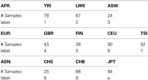
Table 1. 10 subgroups of 607 individuals.
We used all the p = 7,459,664 SNVs appearing in all the three continental groups on chromosomes 1 to 22. In the 7,456,664 SNVs, there are 343,782 rare variants (RVs, with minor allele frequencies, MAFs < 1%), 1,189,061 low frequency variants (LFVs, 1%≤ MAFs < 5%) and 5,926,821 common variants (CVs, MAFs ≥ 5%). There are 132,742, 525,440 and 1,107,080 monomorphic variants in each of the three continental groups: AFR, EUR and ASN, respectively, and there are 18,559 variants that are monomorphic in all the three continental groups. Furthermore, there are 101,279 variants that are monomorphic in AFR but polymorphic in EUR, and 67,661 variants that are monomorphic in AFR but polymorphic in ASN; there are 493,977 variants that are monomorphic in EUR but polymorphic in AFR, and 133,388 variants that are monomorphic in EUR but polymorphic in ASN; there are 1,041,999 variants that are monomorphic in ASN but polymorphic in AFR, and 715,028 variants that are monomorphic in ASN but polymorphic in EUR.
Denote the data by an n × p matrix Z, with rows indexing n individuals, and columns indexing p SNVs. For each SNV, we chose the minor allele as the reference allele. Let Zij ∈ {0, 1, 2} be the number of minor alleles for SNV j of individual i. We centered each column (SNV) to have mean 0; denote the centered data matrix Zc = AZ, where is an n × n centering matrix, I denotes the n × n identity matrix and 1 denotes the length-n vector with each entry equal to 1. Then, we used PCA for dimension reduction (Menozzi et al., 1978; Cavalli-Sforza et al., 1994): we computed the n × n sample covariance matrix H = Zc Ztc, and then used the re-scaled eigenvectors of H as coordinates for subject i, , where λ1 ≥ λ2 ≥ ··· ≥ λJ ≥ 0 are the M largest eigenvalues of H and uj = (uj(1), …, uj(n))t, j ∈ {1, …, J}, are the corresponding eigenvectors. Typically, eigenvectors that correspond to large eigenvalues reveal important ancestry axes.
2.2. Semi-Supervised Spectral Clustering
Existing semi-supervised clustering methods can be categorized into two: search-based and similarity-based. The former is a modified clustering method in that the prior constraints are used to yield appropriate partitions (Demiriz et al., 1999; Wagstaff et al., 2001; Basu et al., 2002). The latter is a clustering method based on a modified similarity metric (Bilenko and Mooney, 2003; Xing et al., 2003; Yang et al., 2008). We think that the latter may be more efficient, since it embeds prior constraints only by simply modifying the similarity metric, while the former may use prior constraints to yield appropriate partitions in each iteration.
With this in mind, in this paper we developed a semi-supervised spectral clustering method to infer population structure. Before proposing this method in detail, we first review some spectral clustering algorithms, which were developed from the studies of weighted graph partitioning problems (Shi and Malik, 2000; Meila and Shi, 2001; Ng et al., 2001; Kannan et al., 2004). The spectral clustering algorithms are similarity-based. A popular choice for defining the similarity between a pair of subjects (xi, xj) (i ≠ j) is letting Wij = exp(−||xi − xj||2/σ2ij), where the scale parameter σij controls the size of local neighborhoods in the weighted graph. Although a global scale σij = σ is often used, as mentioned in Zelnik-manor and Perona (2004), using a local scale parameter, σij = (σiσj)1/2 with σi, σj > 0, for each pair (i, j) may obtain better performance, especially when the clusters of the data have different volumes. Below we review the local scale spectral clustering algorithm proposed by Zelnik-manor and Perona (2004).
Given a set of n points {x1, …, xn} in the J-dimensional Euclidean space RJ and the neighborhood parameter T, cluster them into K clusters as follows:
1. Compute alocal scale σi = d(xi, xiT) for each point xi, where d(.,.) is the Euclidean distance metric and xiT is the T-th nearest neighbor of point xi.
2. Form a weight matrix W with its ij-th element for each i and j ∈ {1, …, n} with i ≠ j and Wii = 0 for each i ∈ {1, …, n}.
3. Define D to be a diagonal matrix with Dii = ∑nj = 1 Wij and construct the normalized Laplacian matrix  = I − D−1/2 WD−1/2.
4. Find u1, …, uK, the smallest K eigenvectors of , and let U be the matrix containing the vectors u1, …, uK as columns.
5. For i = 1, …, n and j = 1, …, K, let U′ij = Uij/(∑Kj′ = 1U2ij′)1/2, and then U′ is a matrix with elements U′ij.
6. For i = 1, …, n, let yi = (y(1)i, …, y(K)i)t ∈ RK be the vector corresponding to the ith row of U′, and then cluster the points {y1, …, yn} with the K-means algorithm into K clusters {S1, …, SK}.
7. Assign the original point xi to cluster Sj if and only if yi is assigned to cluster Sj.
Let  denote the must-link matrix and
  denote the cannot-link matrix for clustering n points {x1, …, xn}, where ii = ii = 0 (i = 1,…,n) and for i ≠ j, ij = 1 (or ij = 1) means that xi, xj are already known to be in the same (or different) cluster(s); ij = 0 (ij = 0) means that we do not know whether xi, xj are in the same cluster. Given the must-link matrix and the cannot-link matrix , Yang et al. (2008) proposed a semi-supervised algorithm by modifying the second step of the local scale spectral clustering algorithm above as follows: for each pair i ≠ j, if ij = 1, then let Wij ≡ 1; if ij = 1, then let Wij ≡ 0. By letting Wij ≡ 1 for a must-link pair (i, j), the algorithm forces the pair (i, j) to be clustered into the same cluster. However, in general, letting Wij ≡ 0 for a cannot-link pair (i, j) may not force the pair (i, j) to be clustered into two different clusters. Wij ≡ 0 only means that observations i and j are far away; if there exists an observation k such that Wik and Wkj are large enough, i and j may still be clustered into one cluster. Thus, for embedding cannot-link information into a spectral clustering algorithm, only letting the weights of all cannot-link pairs to be zero is not enough. To avoid clustering a cannot-link pair (i, j) into one cluster, we adjust Wik and Wkj for each k without any cannot-link information, based on which we propose a new semi-supervised spectral clustering algorithm.
Before introducing the algorithm, to make best use of the semi-supervised information, we may first adjust the must-link matrix and cannot-link matrix as follows: (1) Adjust the must-link matrix such that: for each pair (i, j) (i ≠ j), ij = 1 whenever there exists a k ≠ i, j such that ik = 1 and kj = 1; (2) Adjust the cannot-link matrix such that: for each pair (i, j) (i ≠ j), ij = 1 whenever there exists a k ≠ i, j such that ik = 1 and kj = 1. After the adjustment, if there exists any contradictory pair (i, j) (i ≠ j) with ij = 1 and ik = 1, to avoid being misled we will let ij = 0 and ik = 0.
In fact, though there have been much reported success with using pairwise constraints for clustering, there are two limitations (Davidson and Ravi, 2005; Davidson et al., 2006). First, if the constraints are poorly specified and then using cannot-link constraints may make the feasibility problem intractable (Davidson and Ravi, 2005); second, some constraints may have adverse effects to semi-supervised clustering (Davidson et al., 2006). There were some discussions about how to deal with the limitations, and accordingly some methods were specifically designed to overcome such limitations. Because the concern of the limitations is not the focus of this paper, we will not introduce these methods in detail.
Let V = ∪ij = 1{i, j} and V = ∪ij = 1{i, j}. Now we are ready to show our semi-supervised spectral clustering (SSSC) algorithm.
Algorithm SSSC Given a set of n points 𝒟 = {x1, …, xn} in RJ, a must-link matrix , a cannot-link matrix , and the parameters α ∈ {0, 1}, β ≥ 1 and the neighborhood parameter T, cluster the points into K clusters as follows:
1. Compute the local scale σi = d(xi,xiT) for each point xi, where xiT is the T-th neighbor of point xi.
2. Form the weight matrix W:
a. Initially let for i ≠ j and Wii = 0.
b. For each i and j (i ≠ j), if ij = 1, let Wij = 1; and if ij = 1, let Wij = 0.
c. For each k ∈ V\V, let ck = arg maxc∈V(Wkc). Then for each i ∈ V with cki = 1, let Wik and Wki be replaced by Wik/β.
d. For each k ∈ V\V, let mk = arg maxm∈V(Wkm). If α = 1, then for each j ∈ V with mkj = 1, let Wjk and Wkj be replaced by Wmkk.
3. Define D to be a diagonal matrix with Dii = ∑j Wij and construct the normalized Laplacian matrix = I − D−1/2WD−1/2.
4. Find u1, …, uK, the first K eigenvectors of , and let U be the matrix containing the vectors u1, …, uK as columns.
5. For i = 1, …, n and j = 1, …, K, let U′ij = Uij/(∑Kj′ = 1U2ij′)1/2, and then U′ is a matrix with elements U′ij.
6. For i = 1, …, n, let yi = (y(1)i, … y(K)i)t ∈ RK be the vector corresponding to the ith row of U′, and then cluster the points {y1, …, yn} with the K-means algorithm into K clusters {S1, …, SK}.
7. Assign the original point xi to cluster Sj if and only if yi was assigned to cluster Sj.
Note that in the Step 2.c of our new algorithm above, we believe that for each k ∈ V\V and each cannot-link pair (i, j), if xk is nearer to xi, then it should be much farther away from xj, because the distance between xi and xj has already been set to the maximum. Thus, we penalize the similarity between xk and xj by letting Wjk = Wkj = Wjk/β (β > 1). On the other hand, we set a parameter α to determine whether we force the similarities between a sample k ∈ V\V and a must-link pair (i, j) to be the same. In fact, if α = 0 and β = 1, then our algorithm reduces to that of Yang et al. (2008).
2.3. Choosing the Parameters
We develop a cross-validation procedure to choose the parameters for the Algorithm SSSC, modified from a criterion used in Tibshirani and Walther (2005) for the K-mean clustering. In addition, we borrow the idea of cluster reproducibility index (RI) (Shen et al., 2009) to define a new prediction strength. We summarize the procedure as follows.
Given a data set 𝒟 and a candidate set of parameters Θ = 𝒦 × 𝒜 × ℬ × 𝒯, where 𝒦 and 𝒯 are sets of positive integers, 𝒜 = {0, 1}, and ℬ is a set of real numbers equal to or larger than 1. Randomly permute the sample index set V = [N] of 𝒟, and then partition the permuted sample index set into two roughly equal parts. Select one part as the test index subset Vte for the test data 𝒟te = {Xn: n ∈ Vte} and take the remaining part as the training index subset Vtr for the training data 𝒟tr = {Xn: n ∈ Vtr}. Let tr = VtrVtr, te = VteVte, tr = VtrVtr and te = VteVte. For each θ = (K, α, β, T) ∈ Θ, apply Algorithm SSSC to divide 𝒟tr into K clusters with parameters α, β, T and the must-link matrix tr, the cannot-link matrix tr; apply Algorithm SSSC to divide 𝒟te into K clusters with parameters α, β, T and the must-link matrix te, the cannot-link matrix te. Let ltr and lte denote the corresponding clustering assignments. Divide the test data 𝒟te into K clusters under the guidance of ltr, that is, assign each sample in 𝒟te into the closest cluster of 𝒟tr characterized by ltr in the sense of the Euclidean distance, and then let lte|tr denote the corresponding clustering assignment. Note that here the distance between a sample and a cluster is defined as the minimum distance between this sample and each sample in the cluster. Next, compute the adjusted Rand index (Hubert and Arabie, 1985) between lte|tr and lte as the prediction strength. Repeat the above steps for a number of times with different randomly selected permuted samples, and finally choose with the highest average prediction strength.
Note that while using PCA for dimension reduction in Section 2.1, we did not mention how to choose an appropriate number of PCs. There are many studies about this problem for traditional PCA, such as Jackson (1991), Jolliffe (2002) and Pedro et al. (2005). Because in this paper we only focus on the performance of a clustering algorithm, we propose using a special procedure that is related to the clustering performance. In fact, we view the number of PCs as a parameter and then decide it in the above cross-validation procedure. Especially, we first choose using the above cross-validation procedure for each J in a set of candidate numbers of PCs  , and then choose Ĵ ∈ with the highest average prediction strength among as the best fitted number of PCs.
3. Results
3.1. Main Results
We used all the SNVs appeared in all the three continental groups in chromosomes 1-22 to extract the top t principle components (PCs). As shown in the left panel of Figure 1, the top 2 PCs could completely separate the three continental groups. However, some subgroups could not be completely separated. We used the local scale spectral clustering algorithm introduced in Section Methods to cluster the 607 t-dimension vectors into 10 clusters. As shown in Table 2 and Figure 1, subgroup GBR (‘4’) cannot be completely distinguished from CEU (‘6’); CHS (‘8’) cannot be completely distinguished from CHB (‘9’).
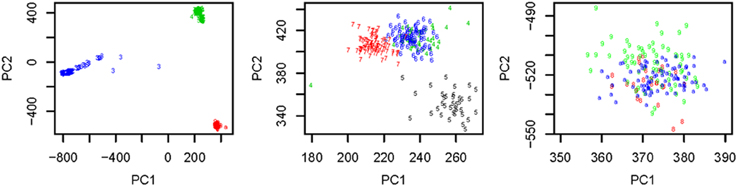
Figure 1. Left: Top: 2 PCs after PCA dimension reduction for the SNV data from chromosomes 1-22, where subjects are self-identified as EUR (green), AFR (blue) and ASN (red). Middle: Top 2 PCs for EUR group: GBR (green), FIN (black), CEU (blue), TSI (red); Right: Top 2 PCs for ASN group: CHS (red), CHB (green), JPT (blue).

Table 2. The numbers of subjects assigned to each of the 10 clusters based on the top 10 PCs using the unsupervised local scale spectral clustering algorithm.
The spectral clustering algorithm used above is an unsupervised clustering algorithm without using any additional clustering information. However, in many cases, partial knowledge is available concerning pairwise (must-link or cannot-link) constraints among a subset of subjects. Thus, we propose a semi-supervised local scale spectral clustering algorithm to make use of the pre-known constraints. We show the performance of our algorithm by varying the number of available must-link or cannot-link constraints. We let SSR denote the semi-supervised ratio, and randomly selected a fraction SSR of individuals from each subgroup. Then we obtained a must-link matrix and a cannot-link matrix according to the selected individuals and their subgroup identities, which were input to our semi-supervised algorithm. We used the algorithm in Yang et al. (2008) and our new proposed algorithm to cluster the 607 individuals into 10 clusters with the top 10, 20, and 30 PCs respectively, and then compared the Rand index (Rand, 1971) and an adjusted Rand (ARand) index (Hubert and Arabie, 1985) between the true subgroups and the clustering results. We repeated this process for 100 times and at each time we randomly selected some individuals for getting the pre-known must-link matrix and cannot-link matrix by setting a different seed in R software. Then we indicated the average results of these 100 simulations in Figure 2. From Figure 2, we can see that when using the top 10, 20 and 30 PCs for clustering, our algorithm performed much better than the existing one with (α = 0, β = 1) (Yang et al., 2008) in terms of the Rand index and adjusted Rand index for almost all the values of SSR. It is clear that the blue vertical lines for our new algorithm appeared with smaller SSR values, indicating that our algorithm made use of the given semi-supervised information more efficiently. In fact, while using other numbers of the top PCs, we also obtained similar results (not shown). Additionally, here in our new algorithm we used α = and β = .
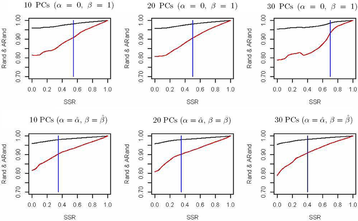
Figure 2. Rand indices (black) and adjusted Rand indices (red) between the true subgroups and the clustering results with various numbers of the top PCs. A vertical blue line indicates the point of SSR, at which the Rand index and adjusted Rand index are both larger than 0.90 for the first time.
Tables 3, 4 present the numbers of subjects assigned to each of the 10 clusters based on the top 10 PCs using the existing SSSC algorithm (α = 0, β = 1) (Yang et al., 2008) and our Algorithm SSSC with SSR = 0.5. We can see that our new algorithm performed much better than the existing one.
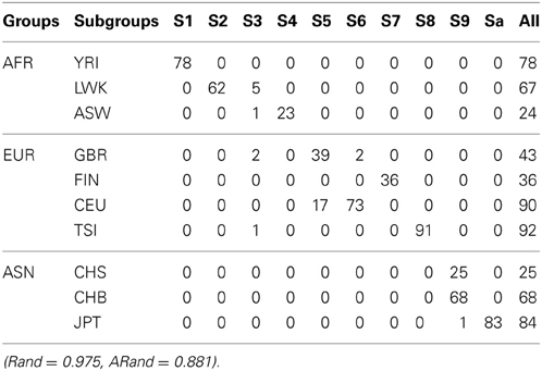
Table 3. The numbers of subjects assigned to each of the 10 clusters based on the top 10 PCs using the existing SSSC algorithm (α = 0, β = 1) with SSR = 0.5.
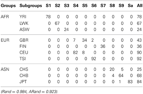
Table 4. The numbers of subjects assigned to each of the 10 clusters based on the top 10 PCs using our new SSSC algorithm (α = , β = ) with SSR = 0.5.
To further illustrate the difference among the unsupervised local scale spectral clustering algorithm, the existing SSSC algorithm (α = 0, β = 1) (Yang et al., 2008) and our new SSSC algorithm (α = , β = ), we plotted the first two co-ordinates (of yi's in Step 6) for each of the three algorithms (see Figure 3). To better observe the separation between the two subgroups CHS (‘8’) and CHB (‘9’), we particularly plotted for the two subgroups, where the colors of the subjects in CHB were still kept red, however, those in CHS were changed to black (see the right three sub-figures of Figure 3). The top two sub-figures are for the unsupervised local scale spectral clustering algorithm, the middle two are for the existing SSSC algorithm (α = 0, β = 1) and the bottom two are for our SSSC algorithm (α = , β = ). From the first two sub-figures of Figure 3 and Table 2, we see that the two pairs of subgroups, GBR-CEU and CHS-CHB were inseparable, respectively. Then for the middle two sub-figures of Figure 3 and Table 3, by adjusting the similarities between must-link pairs to be 1 and those between cannot-link pairs to be 0, the subjects in GBR and CEU were a little more separable, however the subjects in CHS and CHB were still inseparable. Finally for the last two sub-figures of Figure 3 and Table 4, we can see that the subjects in all the subgroups were more separable, and in particular, in the bottom right sub-figure the subjects in CHS and CHB were more separable.
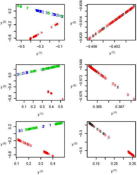
Figure 3. The top two sub-figures are for the unsupervised local scale spectral clustering algorithm, the middle two are for SSSC algorithm (α = 0, β = 1) and the bottom two are for our SSSC algorithm (α = , β = ). Note that in the right three sub-figures, the colors of the subjects in CHS (‘8’) were changed from red to black. Note that the y(1) and y(2) axes are just the first two co-ordinates of the data points {y1, …, yn} in Step 6 of Algorithm SSSC.
3.2. Semi-Supervised Clustering Versus Classification
We also did some numerical experiments to compare classification (supervised learning) with our semi-supervised clustering. For illustration and to have a easier problem for classification, we only took the individuals in the EUR continental group and used common variants (CVs) with minor allele frequencies (MAFs) greater than 5% on chromosome 1. Furthermore, we used PLINK (Purcell et al., 2007) to prune out correlated SNVs with a sliding window of size 50 (shifted by 5) and a threshold of r2 ≤ 0.05, after which we had 11,840 CVs.
First, we randomly chose a fraction SSR of individuals from each of the above four subgroups as semi-supervised information for our clustering algorithm and as the training data for a classification algorithm. We used penalized multinomial logistic regression with the Lasso or the Ridge penalty for classification; the penalization parameter was chosen by 5-fold cross-validation. We used the trained classifier to predict the subgroup labels for the remaining data, and combined the known labels in the training data and the predicted labels in the test data together to compare with the true labels in terms of the Rand indices and adjusted Rand indices. The top two sub-figures in Figure 4 summarize the corresponding results based on 100 simulations; it is demonstrated that in our experiments, our semi-supervised clustering algorithm performed much better than both Lasso- and Ridge-penalized regression, especially for cases with low SSRs.
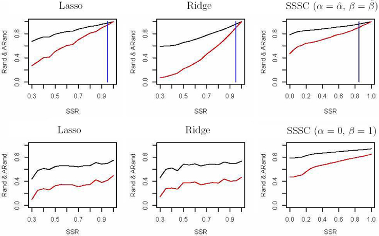
Figure 4. Rand indices (black) and adjusted Rand indices (red) between the true subgroups and the SSSC or classification results. A vertical blue line indicates the point of SSR, at which the Rand and adjusted Rand are both bigger than 0.90 for the first time. The top three sub-figures demonstrate comparison of Lasso, Ridge and SSSC for the cases that semi-supervised information involves all the four subgroups, while the bottom three for the cases that semi-supervised information involves two subgroups.
On the other hand, in some cases the given semi-supervised information may not involve all the four subgroups. For example, we only had information about a subset of subjects from the CEU and GBR subgroups, but not any from the other subgroups. As before, we randomly selected a fraction (SSR) of individuals from the CEU and GBR subgroups respectively; they were used as semi-supervised information for our algorithm and as training data for a classification algorithm. The bottom three sub-figures in Figure 4 show the corresponding comparisons, indicating that our semi-supervised clustering algorithm performed overwhelmingly better than Lasso- and Ridge-penalized regression, because the classification algorithm predicted all the individuals of the unknown TSI or FIN subgroup as of either CEU or GBR subgroup. This illustrates an obvious advantage of a semi-supervised clustering approach for discovery of novel classes.
4. Discussion
4.1. Dimension Reduction
In Section 3, we have demonstrated good performance of our algorithm with a few top PCs. In addition, we also obtained similar results (not shown) with other methods for dimension reduction, such as the spectral graph approach used in SpectralR and SpectralGEM (Lee et al., 2010). We used the spectral method in (Lee et al., 2010) for dimension reduction, then clustered the data into 10 clusters; we took the same procedure to compare the Rand index and adjusted Rand index values. Figure 2.
4.2. All or a Subset of SNVs?
In the previous section, we used all 7,459,664 SNVs appearing in all the three continental groups on chromosomes 1 to 22 without pruning out SVNs in linkage disequilibrium. We used common variants (CVs) with minor allele frequencies (MAFs) greater than 5% on chromosomes 1 to 22, and used PLINK (Purcell et al., 2007) to prune out correlated SNVs with a sliding window of size 50 (shifted by 5) and a threshold of r2 ≤ 0.5, after which we had 1,022,090 CVs. Next, we used PCA for dimension reduction and then use the three algorithms to analyze the resulting data after dimension reduction.
Tables 5–7 present the numbers of subjects assigned to each of the 10 clusters based on the top 10 PCs using the unsupervised spectral clustering algorithm, the existing semi-supervised spectral clustering algorithm and our new algorithm with SSR = 0.5. From these results and those indicated by Tables 2–4, we see that using all the SNVs was better than using the pruned data in terms of the performance of the unsupervised spectral clustering. For the two semi-supervised spectral clustering algorithms, we find that while using the pruned data, the new semi-supervised spectral clustering algorithm still performed better than the existing one (Yang et al., 2008) as in Section 3.1 with all the SNVs.
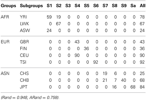
Table 5. The numbers of subjects assigned to each of the 10 clusters based on the top 10 PCs using the unsupervised local scale spectral clustering algorithm.
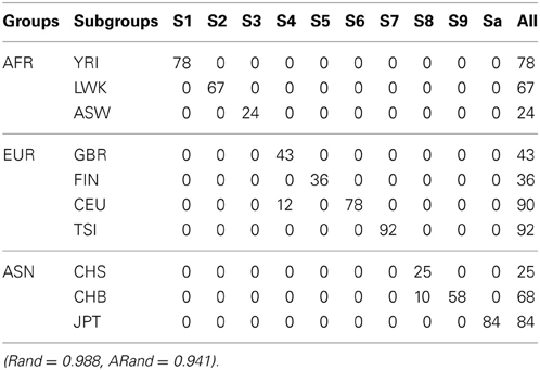
Table 6. The numbers of subjects assigned to each of the 10 clusters based on the top 10 PCs using the existing SSSC algorithm (α = 0, β = 1) with SSR = 0.5.
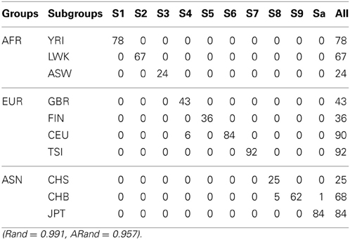
Table 7. The numbers of subjects assigned to each of the 10 clusters based on the top 10 PCs using our new SSSC algorithm (α = , β = ) with SSR = 0.5.
4.3. Local Scale Spectral Clustering
Our semi-supervised spectral clustering algorithm is based on the local scale spectral clustering (Zelnik-manor and Perona, 2004), because we believe that local scales work better than choosing a single global scale for all pairs of subjects. In some situations the subgroups might not have the same scale; from our experience, given a fixed number of clusters, the subjects in a sparser group are more likely to be divided into more clusters, and the individuals in a denser group are more likely to be merged together. In these cases, it will be difficult to choose a suitable single global scale. In contrast, using local scales automatically adjusts for the heterogeneous scales in the subgroups. We did some experiments to compare the spectral clustering algorithms with a global scale and with local scales. We used several candidate values for a global scale, and found that even the best clustering result (in terms of the Rand indices and adjusted Rand indices) was almost the same as that obtained by using local scales. Because it is not the main point of this study, we do not show the detailed comparisons here.
5. Conclusions
We have proposed a new semi-supervised spectral clustering algorithm based on a more efficient use of the cannot link constraints in prior data. A whole-genome sequencing dataset from the 1000 Genomes Project was analyzed to compare the performance of our and other algorithms. In our experiments, unsupervised clustering algorithms could not completely separate some subgroups, such as the CEU-GBR and CHB-CHS subgroups; our semi-supervised spectral clustering algorithm, along with a subset of individuals with known subgroup identities, distinguished these subgroups much better. Our proposed method may be potentially useful in genetic association studies. Its extensions to other clustering (Thalamuthu et al., 2006) and dimension reduction approaches are to be studied.
Conflict of Interest Statement
The authors declare that the research was conducted in the absence of any commercial or financial relationships that could be construed as a potential conflict of interest.
Acknowledgments
Funding: This work was supported by NIH grants R01GM081535, R01-HL65462 and R01-HL105397, by NSF grants DMS-0906616 and DMS-1207771, and by NSFC grant 11101182.
References
Basu, S., Banerjee, A., and Mooney, R. J. (2002). “Semisupervised clustering by seeding,” in Proceedings of 19th International Conference on Machine Learning, (San Francisco, CA), 27–34.
Bilenko, M., and Mooney, R. J. (2003). “Adaptive duplicate detection using learnable string similarity measures,” in Proceedings of the 9th ACM SIGKDD International Conference on Knowledge Discovery and Data Mining, (Washington, DC), 39–48. doi: 10.1145/956750.956759
Cavalli-Sforza, L., Menozzi, P., and Piazza, A. (1994). The History and Geography of Human Genes, Princeton, NJ: Princeton Univ. Press.
Davidson, I., Basu, S., and Wagstaff, K. (2006). “Measuring constraint-set utility for partitional clustering algorithms,” in Proceedings of the Tenth European Principles and Practice of KDD (PKDD), (Berlin).
Davidson, I., and Ravi, S. (2005). “Clustering with constraints: feasibility issues and the k-means algorithm,” in Proceedings of the 2005 SIAM International Conference on Data Mining (SDM-05), (Newport Beach, CA).
Demiriz, A., Bennett, K. P., and Embrechts, M. J. (1999). Semi-supervised clustering using genetic algorithms. Artif. Neural Netw. Eng. 809–814.
Devlin, B., Bacanu, S. A., and Roeder, K. (2004). Genomic control to the extreme. Nat. Genet. 36, 1129–1130. doi: 10.1038/ng1104-1129.
Devlin, B., and Roeder, K. (1999). Genomic control for association studies. Biometrics 55, 997–1004. doi: 10.1111/j.0006-341X.1999.00997.x
Grira, N., Crucianu, M., and Boujemaa, N. (2004). “Unsupervised and Semi-supervised Clustering: a brief survey,” in A Review of Machine Learning Techniques for Processing Multimedia Content, Report of the MUSCLE European Network of Excellence (FP6).
Hirschhorn, J. N., and Daly, M. J. (2005). Genome-wide association studies for common diseases and complex traits. Nat. Rev. Genet. 6, 95–108. doi: 10.1038/nrg1521
Hubert, L., and Arabie, P. (1985). Comparing partitions. J. Classif. 2, 1993–1218. doi: 10.1007/BF01908075
International HapMap Consortium. (2003). The international HapMap project. Nature 426, 789–796. doi: 10.1038/nature02168
Kannan, R., Vempala, S., and Vetta, V. (2004). On spectral clustering-good, bad and spectral. J. ACM 51, 497–515.
Lander, E. S., and Schork, N. J. (1994). Genetic dissection of complex traits. Science 265, 2037–2048. doi: 10.1126/science.8091226
Lee, C., Abdool, A., and Huang, C. H. (2009). PCA-based population structure inference with generic clustering algorithms. BMC Bioinformatics 10(Suppl. 1):S73. doi: 10.1186/1471-2105-10-S1-S73
Lee, A. B., Luca, D., and Roeder, K. (2010). A spectral graph approach to discovering genetic ancestry. Ann. Appl. Stat. 4, 179–202. doi: 10.1214/09-AOAS281
Marchini, J., Cardon, L. R., Phillips, M. S., and Donnelly, P. (2004). The effects of human population structure on large genetic association studies. Nat. Genet. 36, 512–517. doi: 10.1186/1471-2156-6-S1-S109
Meila, M., and Shi, J. (2001). Learning segmentation by random walks, Adv. Neural Inf. Process. Syst. 470–477.
Menozzi, P., Piazza, A., and Cavalli-Sforza, L. (1978). Synthetic maps of human gene frequencies in Europeans. Science 201, 786–792. doi: 10.1126/science.356262
Ng, A. Y., Jordon, M. I., and Weiss, Y. (2001). On spectral clustering: analysis and an algorithm. Adv. Neural Inf. Process. Syst. 14, 849–856.
Paschou, P., Lewis, J., Javed, A., and Drineas, P. (2010). Ancestry informative markers for fine-scale individual assignment to worldwide populations. J. Med. Genet. 47, 835–847. doi: 10.1136/jmg.2010.078212
Patterson, N., Price, A. L., and Reich, D. (2006). Population structure and eigen analysis. PLoS Genet. 2:e190. doi: 10.1371/journal.pgen.0020190
Pedro, R. P.-N., Donald, A. J., and Keith, M. S. (2005). How many principal components? Stopping rules for determining the number of non-trivial axes revisited. Comput. Stat. Data Anal. 49, 974–997. doi: 10.1016/j.csda.2004.06.015
Pritchard, J. K., Stephens, M., Rosenberg, N. A., and Donnelly, P. (2000). Association mapping in structured populations, Am. J. Hum. Genet. 67, 170–181. doi: 10.1086/302959
Purcell, S., Neale, B., Todd-Brown, K., Thomas, L., Ferreira, M., Bender, D., et al. (2007). PLINK: a tool set for whole-genome association and population-based linkage analysis. Am. J. Hum. Genet. 81, 559–575. doi: 10.3410/f.1162373.622875
Purcell, S., and Sham, P. (2004). Properties of structured association approaches to detecting population stratification. Hum. Hered. 58, 93–107. doi: 10.1159/000083030
Rand, W. M. (1971). Objective criteria for the evaluation of clustering methods. J. Am. Stat. Associat. 66, 846–850. doi: 10.2307/2284239
Satten, G. A., Flanders, W. D., and Yang, Q. (2001). Accounting for unmeasured population substructure in case-control studies of genetic association using a novel latent-class model. Am. J. Hum. Genet. 68, 466–477. doi: 10.1086/318195
Shen, R., Olshen, A. B., and Ladanyi, M. (2009). Integrative clustering of multiple genomic data types using a joint latent variable model with application to breast and lung cancer subtype analysis. Bioinformatics 22, 2906–2912. doi: 10.1093/bioinformatics/btp543
Shi, J., and Malik, J. (2000). Normalized cuts and image segmentation. IEEE Trans. Pattern Anal. Mach. Intell. 22, 888–905. doi: 10.1109/34.868688
Tibshirani, R. (1996). Regression shrinkage and selection via the lasso. J. R. Stat. Soc. Ser. B 58, 267–288.
Tibshirani, R., and Walther, G. (2005). Cluster validation by prediction strength. J. Comput. Graph. Stat. 14, 511–528. doi: 10.1198/106186005X59243
Thalamuthu, A., Mukhopadhyay, I., Zheng, X., and Tseng, G. C. (2006). Evaluation and comparison of gene clustering methods in microarray analysis. Bioinformatics 22, 2405–2412. doi: 10.1093/bioinformatics/btl406
Thomas, D. C., Haile, R. W., and Duggan, D. (2005). Recent developments in genomewide association scans: a workshop summary and review. Am. J. Hum. Genet. 77, 337–345. doi: 10.1086/432962
Wagstaff, K., Cardie, C., Rogers, S., and Schroedl, S. (2001). “Constrained K-Means clustering with background knowledge.” in Proceedings of 18th International Conference on Machine Learning, 577–584.
Xing, E. P., Ng, A. Y., Jordan, M. I., and Russel, S. (2003). Distance metric learning, with application to clustering with side-information. Adv. Neural Inf. Process. Sys. 15, 505–512.
Yang, C., Zhang, X., Jiao, L., and Wang, G. (2008). Self-tuning semi-supervised spectral clustering. Comput. Intell. Secur. 1, 1–5. doi: 10.1109/CIS.2008.141
Zelnik-manor, L., and Perona, P. (2004). Self-tuning spectral clustering. Adv. Neural Inf. Process. Syst. 17, 1601–1608.
Zhang, Y., Guan, W., and Pan, W. (2012). Adjustment for population stratification via principal components in association association analysis of rare variants. Genet. Epidemiol. 37, 99–109. doi: 10.1002/gepi.21691
Keywords: clustering, genome-wide association studies (GWAS), population stratification, semi-supervised spectral clustering, single nucleotide variant (SNV)
Citation: Liu B, Shen X and Pan W (2013) Semi-supervised spectral clustering with application to detect population stratification. Front. Genet. 4:215. doi: 10.3389/fgene.2013.00215
Received: 04 August 2013; Paper pending published: 29 August 2013;
Accepted: 04 October 2013; Published online: 25 October 2013.
Edited by:
Shuang Wang, Columbia University, USAReviewed by:
Weihua Guan, University of Minnesota, USARen-Hua Chung, National Health Research Institutes, Taiwan
Copyright © 2013 Liu, Shen and Pan. This is an open-access article distributed under the terms of the Creative Commons Attribution License (CC BY). The use, distribution or reproduction in other forums is permitted, provided the original author(s) or licensor are credited and that the original publication in this journal is cited, in accordance with accepted academic practice. No use, distribution or reproduction is permitted which does not comply with these terms.
*Correspondence: Wei Pan, Division of Biostatistics, School of Public Health, University of Minnesota, A460 Mayo Building, MMC 303, Minneapolis, MN 55455, USA e-mail: weip@biostat.umn.edu