 Arne B. Gjuvsland
 Yunpeng Wang
 Erik Plahte
 Stig W. Omholt2,3
- 1Centre for Integrative Genetics (CIGENE), Department of Mathematical Sciences and Technology, Norwegian University of Life Sciences, Ås, Norway
- 2Centre for Integrative Genetics (CIGENE), Department of Animal and Aquacultural Sciences, Norwegian University of Life Sciences, Ås, Norway
- 3Department of Biology, Centre for Biodiversity Dynamics, NTNU Norwegian University of Science and Technology, Trondheim, Norway
It was recently shown that monotone gene action, i.e., order-preservation between allele content and corresponding genotypic values in the mapping from genotypes to phenotypes, is a prerequisite for achieving a predictable parent-offspring relationship across the whole allele frequency spectrum. Here we test the consequential prediction that the design principles underlying gene regulatory networks are likely to generate highly monotone genotype-phenotype maps. To this end we present two measures of the monotonicity of a genotype-phenotype map, one based on allele substitution effects, and the other based on isotonic regression. We apply these measures to genotype-phenotype maps emerging from simulations of 1881 different 3-gene regulatory networks. We confirm that in general, genotype-phenotype maps are indeed highly monotonic across network types. However, regulatory motifs involving incoherent feedforward or positive feedback, as well as pleiotropy in the mapping between genotypes and gene regulatory parameters, are clearly predisposed for generating non-monotonicity. We present analytical results confirming these deep connections between molecular regulatory architecture and monotonicity properties of the genotype-phenotype map. These connections seem to be beyond reach by the classical distinction between additive and non-additive gene action.
Introduction
Quantitative genetics is the major theoretical foundation for genetic studies in production biology, evolutionary biology, and biomedicine. A core concept in quantitative genetics is the genotypic value, the mean observed phenotype for a given genotype. It constitutes the basis for the genotype-to-phenotype (GP) map concept. The shape of a given GP map is typically described by the classical gene action terms: additivity, dominance, and epistasis. Together with genotype frequencies in a given population, the GP map is the basis for decomposing observed phenotypic variance into environmental variance and genetic variance components including additive variance, dominance variance and epistatic variance. This provides the basis for a very successful theory when it comes to predicting selection response and breeding values (Falconer and Mackay, 1996; Lynch and Walsh, 1998) and more recent statistical genetics methods for mapping Quantitative Trait Loci (QTL) (Neale et al., 2008). Quantitative genetics thus provides a mature machinery for predicting the population level consequences of a given GP map, but in order to understand several generic genetic phenomena there is a stated need for new tools for disclosing how the shape of the GP map is determined by underlying biology (Jaeger et al., 2012; Moore, 2012; Gjuvsland et al., 2013).
One such phenomenon is the resemblance between parents and offspring. An explanation in quantitative genetic terms is that the additive variance (VA) makes up a substantial part of the phenotypic (VP) and genetic variance (VG). Hill et al. (2008) showed that in populations with extreme allele frequencies, high VA/VG ratios will arise regardless of the shape of the GP map. However, for populations with intermediate allele frequencies a much wider range of VA/VG ratios is observed (Wang et al., 2013). In such populations, high VA/VG ratios cannot be fully accounted for without considering properties of the GP map. Gjuvsland et al. (2011) showed that a key feature of GP maps that give high ratios of additive to genotypic variance (VA/VG), is a monotone (or order-preserving) relation between gene content (the number of alleles of a given type) and phenotype. This led to the hypothesis that the regulatory circuitry of sexually reproducing organisms predominantly predisposes for highly monotone genotype-phenotype maps.
Here we address the above hypothesis by a two-step approach. First we provide methods and software tools for measuring monotonicity of generic GP maps (i.e., sets of genotypic values). Then we use these tools on the data generated by an extensive simulation study of a broad collection of gene regulatory network models. In these network models the steady state expression levels serve as phenotypes and genetic variation is introduced through parameters describing maximal production rates and the shape of the gene regulation function. Such causally cohesive genotype-phenotype (cGP) models [see Gjuvsland et al. (2013) and references therein] allow us to identify relationships between regulatory network architecture and properties of the resulting GP maps.
Our results confirm the prediction that the GP maps arising from a wide range of gene regulatory network motifs are in general highly monotone. In addition we show through numerical as well as mathematical analysis that regulatory motifs involving incoherent feed-forward or positive feedback stand out in their capacity to generate non-monotonicity. These relationships between molecular regulatory architecture and properties of the genotype-phenotype map—of substantial relevance to functional genomics in general—are beyond reach by the standard distinction between additive and non-additive gene action.
Our approach can be applied to cGP models of a wide range of biological systems at any level of model complexity. It opens for a systematic study of the monotonicity properties of molecular regulatory structures underlying the whole spectrum of physiological regulation. This suggests that the concept of monotonicity of GP maps can be used to build theory about heredity phrased in terms of molecular mechanism, something which standard genetic concepts and approaches appear to be incapable of.
Models and Methods
Background on Monotonicity of GP Maps
To ease understanding we provide a brief recapitulation of the concept of monotonicity (or order-preservation) in GP maps introduced in (Gjuvsland et al., 2011). We consider a diploid genetic model with N biallelic loci (alleles indexed 1 and 2) underlying a quantitative phenotype. A genotype at a single locus k is denoted by gk ∈ {11, 12, 22}. In the case of two loci k and l there are 9 possible genotypes gkl = gkgl ∈ {1111, 1112, 1122, 1211, …, 2212, 2222}. The general N loci genotype space Γ contains 3N genotypes g1g2 … gN (in condensed notation g1:N) constructed by concatenating single locus genotypes, Γ = {g1g2 … gN | gk ∈ {11, 12, 22}, k = 1, 2, …, N}. For any locus k, the genotypic background, i.e., the allele composition of all loci except k, is g(k) = g1g2 … gk − 1 gk + 1 … gN = g1: k − 1 gk + 1: N. For example, if N = 4 then g(2) = 112212 means that the genotypes of locus 1, 3, and 4 are 11, 22, and 12, respectively. We use the straightforward notation g1 g2 … gk − 1 11gk + 1 … gN = g1:k − 1 11gk + 1: N to indicate a genotype where gk = 11 while the background genotype is arbitrary. We will also use the compressed notation 11g(k) (or generally gkg(k)).
We use the 2-allele content (i.e., the number of 2-alleles) of genotypes to define a partial order on the genotype space Γ (see Figure 1, left panel for an illustration). For a particular locus k we order the three genotypes sharing the same background genotype g1: k − 1 gk + 1: N as follows,
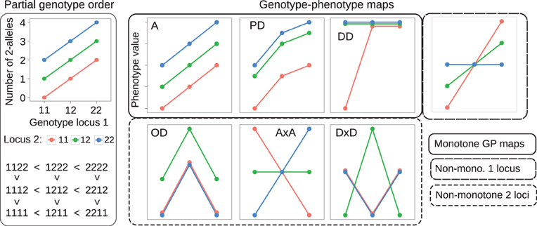
Figure 1. Examples of partial genotype order and genotype-phenotype maps. Left panel: The allele content defines a partial order on genotype space. A two-locus example is shown. The plot at the top displays the genotype at locus 1 (x-axis) and locus 2 (color) vs. the total number of 2-alleles (y-axis) in the two-locus genotype. The resulting partial ordering of genotypes is shown below. Right panel: Each lineplot shows the 9 genotypic values (y-axis) for a single GP map, coding of genotype are the same as in the left panel. GP maps that preserve the partial order of genotypes are called monotone. Examples shown are an intra- and interlocus additive map (A), a map showing partial dominance at both loci (PD), and duplicate dominant (DD) epistasis (see Table 1 in Phillips, 1998). GP maps that break the partial order of genotypes are called non-monotone, examples shown are pure overdominance at both loci (OD), additive-by-additive epistasis (A × A) and dominance-by-dominance epistasis (D × D). The rightmost plot shows a GP map that is monotone w.r.t. locus 1, but non-monotone w.r.t. locus 2.
We call this the partial genotype order relative to locus k, and it defines a strict partial order on Γ.
A genotype-phenotype map is a mapping G that assigns to each genotype g ∈ Γ a real-valued genotypic value G(g) (the mean trait value for a given genotype). We define monotonicity of G in terms of how it transforms the partial genotype order to the algebraic order of the genotypic values G(g). Without loss of generality we assume that the allele indexes at each locus have been chosen such that G(1111 … 11) is the smallest of all homozygote genotypic values. We call a genotype-phenotype map G monotone or order-preserving with respect to locus k if it preserves the partial genotype order relative to locus k, i.e., if,
for all genetic backgrounds of locus k. By allowing non-strict inequalities we include GP maps showing complete dominance and complete magnitude epistasis (Weinreich et al., 2005) in the class of order-preserving GP maps. Conversely we call a GP map non-monotone or order-breaking with respect to locus k if it does not preserve the partial genotype order relative to locus k for all backgrounds. Figure 1 (right panel) shows classical dominance and epistasis patterns, categorized into monotone and non-monotone GP maps.
Statistical Decomposition of Genotype-Phenotype Maps
Given a genotype-phenotype map G as described above and a corresponding vector of genotype frequencies f in a population, quantitative genetic provides methods for orthogonal decomposition of genotypic values and resulting genetic variance in the population into additive and non-additive (dominance and epistasis) components (Lynch and Walsh, 1998). We performed such statistical decomposition with the function linearGPmapanalysis in the R package noia (http://cran.r-project.org/package=noia; Le Rouzic and Alvarez-Castro, 2008) version 0.94.1. We assumed an idealized population where all genotype frequencies are equal (1/3N). In such a hypothetical population the NOIA (Alvarez-Castro and Carlborg, 2007) statistical and functional formulations and the unweighted regression model proposed by Cheverud and Routman (1995) are equivalent. Furthermore, the decomposition of genotypic values is equivalent to decomposing G into a sum of additive and non-additive GP maps, and the genetic variance in this case is simply the variance of the 3N genotypic values in G. We used the NOIA statistical formulation to decompose a GP map G into its additive and non-additive components, and computed the ratio of additive to total genetic variance VA/VG as a measure of how well the additive component describes the original GP map. In case of the illustrative GP maps depicted in Figure 1, this gives VA/VG = 1 for the fully additive GP map A, and VA/VG = 0 for the pure overdominance (OD) and the pure epistasis (Cheverud and Routman, 1996) maps A × A and D × D.
Gene Regulatory Network Models
Gene expression in eukaryotes is controlled through gene regulatory networks involving numerous regulatory mechanisms [see e.g., Latchman (2005), for details]. Modeling of such gene regulatory networks is well-established, and available modeling frameworks range from coarse-grained descriptions of the topology of genome-wide networks to very detailed mechanistic models describing the dynamics of small networks (De Jong, 2002; Schlitt and Brazma, 2007; Karlebach and Shamir, 2008). In line with a large number of authors we used ordinary differential equations (ODEs) to study a family of generic gene regulatory network models containing three diploid genes X1, X2, and X3, organized as a regulatory system where the rate of expression of each gene can be regulated by the expression level of one or both of the other genes. The wiring of the system is described by a 3 × 3 connectivity matrix A with elements Akl ∈ {−1, 0, 1}. The signs of the elements of A describe the mode of regulation, Akl = 0 indicates that Xl is not a regulator of Xk, if Akl = 1 then Xl is an activator of Xk, and if Akl = −1 then Xl is a repressor of Xk. Gene regulatory systems are often laid out visually as signed directed graphs. There is a one-to-one correspondence between a connectivity matrix and a signed directed graph, two examples are illustrated in Figure 4. We used the sigmoid formalism (Mestl et al., 1995; Plahte et al., 1998) in the diploid form (Omholt et al., 2000) where the expression the two alleles of gene k is described by the following ODEs,
Here αki is the maximal production rate for allele i of gene Xk, γki is the decay rate, while Rki is the gene regulation function (dose-response function). If Xk has no regulators, we assume production is always switched on i.e., Rki = 1. If Xk has a single regulator Xl, the gene regulation function is given as Rki(yl) = S(yl, θlki, plki), where S(y, θ, p) = yp/(yp + θp) if Xl is an activator and S(y, θ, p) = 1 − yp/(yp + θp) if it is a repressor. In both cases the parameter θlki gives the amount of regulator needed to get 50% of maximal production rate, and plki determines the steepness of the response. In the case of two regulators Xl and Xj we set Rki(yl, yj) = S(yl, θlki, plki)S(yj, θjki, pjki), corresponding to the Boolean AND function. Modeling transcription regulation by means of Hill functions and Boolean composition has a long tradition in modeling of gene regulation and is widely used.
With three genes and up to two regulators per gene the number of possible connectivity matrices is 6859. We further required that the system is connected, and that X3 is downstream to both X1 and X2 so either X1 and X2 both regulate X3 directly (A31A32 ≠ 0), or one of them regulates X3 directly and the other one indirectly (A31A12 ≠ 0 or A32A21 ≠ 0). This reduces the number of distinct connectivity matrices to 3724. Finally, we identified pairs of matrices that are symmetric with respect to interchanging X1 and X2 and picked just one matrix from each pair. The resulting 1881 connectivity matrices were used for our gene regulatory simulations.
Identifying Feedback Loops and Feedforward Motifs
Feedback and feedforward motifs appear recurrently as regulatory building blocks in transcription networks across all living organisms. These network motifs have several characteristic features (Alon, 2007), negative feedback can for example accommodate fast transcriptional responses and homeostasis, while positive feedbacks are utilized as biological switches. We went through all 1881 gene regulatory models and extracted information about their feedback and feedforward loop characteristics from their connectivity matrices. For each system we computed three autoregulatory feedback loop products FL1 = A11, FL2 = A22, FL3 = A33, three two-gene feedback loop products: FL12 = A21A12, FL13 = A31 A13, FL23 = A23 A32 and two three-gene feedback loop products: FL123 = A32 A21 A13, FL213 = A31 A12A23. Non-zero loop products indicate that the system contains the corresponding feedback loop, and the sign of the loop product gives the sign of the feedback loop. We also computed the products for two feedforward motifs: FFL32 = A32(A31 A12), FFL31 = A31 (A32A21). Again non-zero products indicate that the system contains the corresponding feedforward motif, a positive value corresponds to a coherent feedforward while a negative value indicates incoherent feedforward. Figure 4 depicts the connectivity matrix and the signed digraphs of a system with a positive feedback loop as well as a system with incoherent feedforward. Spreadsheet S1 contains adjacency matrices and loop products for all 1881 motifs.
Gene Regulatory Network Simulations
The simulation were performed with the Python package cgptoolbox (http://github.com/jonovik/cgptoolbox), using the sigmoidmodel submodule, which contains an implementation of the gene regulatory network model (Equation 3) and the connectivity matrix A. A similar simulation setup is found in Gjuvsland et al. (2011) together with a discussion of gene regulation functions and the genotype-parameter map in molecular terms. We compared two different types of genotype-to-parameter maps:
- Genotype to parameter map without pleiotropy: biallelic genotypic variation for all three loci was introduced through the maximal production rates αki. For each Monte Carlo simulation the allelic parameter values were sampled from U(100, 200).
- Genotype to parameter map with pleiotropy: allelic parameter values were sampled for maximal production rates αki (sampled from U(100, 200)), regulation thresholds θlki (sampled from U(20, 40)), and regulation steepnesses plki (sampled from U(1, 10)).
All decay rates γki were set equal to 10. We assembled parameter sets for all 27 diploid genotypes, and for each genotypic parameter set the system of Equation 3 was integrated numerically until convergence to a stable state. The equilibrium value of y3 was recorded as phenotype. Datasets where the system failed to converge for one or more genotypes were discarded. For each of the 1881 motifs we performed 1000 Monte Carlo simulations.
Some Monte Carlo simulations lead to very little phenotypic variation, in the sense that the span between the largest and smallest of the 27 genotypic values was small. In order to avoid artifacts arising from the numeric ODE solver tolerance, these essentially flat GP maps were discarded. Further analysis of monotonicity and variance components were only performed on GP maps where the absolute range (maximum genotypic value – minimum genotypic value) and relative range (absolute range/mean genotypic value) were both > 0.01.
Results
Measuring Monotonicity of GP Maps
In the following we present two numerical measures for quantifying monotonicity in a GP map G with N biallelic loci. The first quantifies the monotonicity for individual loci by comparing negative and positive allele substitution effects before weighting the individual loci into an overall measure. The second utilizes isotonic regression to quantify the distance between G and the closest fully monotone GP map.
Measure 1: quantifying non-monotonicity by substitution effects
We first develop a measure of monotonicity based on the effects of substituting a single allele at locus k,
while keeping the background genotype g(k) = g1: k + 1gk + 1: N fixed. Monotonicity as defined by Equation 2 is equivalent to si (g(k)) ≥ 0 for i = 1, 2 across all genetic backgrounds of locus k. By taking into account also the magnitude of the substitution effects we can quantify the deviation from strict monotonicity. We start with the set Sk = {si(g(k))} of single allele substitution effects for locus k for i = 1, 2 and across all genotypic backgrounds g(k). The total number of elements in Sk thus becomes 2· 3N − 1, and we split the set into two disjoint subsets reflecting their sign; Sk+ = {si(g(k)) ∈ Sk | si (g(k)) > 0} and Sk− = {si (g(k)) ∈ Sk | si (g(k)) < 0}. We compute the sum of positive substitution effects and the sum of absolute values of negative substitution effects,
and let Tk = Pk + Nk denote the overall sum of absolute substitution effects. We then define the degree to which the GP map G is monotone with respect to locus k by,
The absolute value in the numerator ensures that the measure mk is invariant with respect to the choice of indexes for the two alleles of locus k. Interchanging the numbering of the alleles leads to the mappings s1 (g(k)) ↦ −s2(g(k)), s2(g(k)) ↦ −s1 (g(k)), which leaves the value of mk unchanged. By the triangle inequality mk ≤ 1. If mk = 1, then G is monotonic with respect to locus k, whereas mk < 1 implies that G is order-breaking w.r.t. locus k. If mk = 0, then the positive substitution effects equal the negative substitution effects in magnitude and we say that G is completely order-breaking w.r.t. locus k. This measure distinguishes well between the monotone and non-monotone maps in Figure 1. Clearly m1 = m2 = 1 for the additive map (A) and GP maps showing partial dominance and duplicate dominance epistasis. In contrast, m1 = m2 = 0 for the maps showing pure OD and pure epistasis (A × A and D × D).
In order to quantify the overall monotonicity of the GP map G we introduce the degree of monotonicity (m) which is a weighted mean of all mk, where the weights reflect the relative effect size of the loci in terms of Tk,
As shown in Figure 3A, the degree of monotonicity is accordingly 1 for the monotone maps in Figure 1 while it is 0 for the pure OD and pure epistasis maps. This definition of degree of monotonicity allows us to establish a vocabulary that is analogous to the classification of single locus dominance; i.e., a GP map is called monotone if m = 1, (partially) non-monotone if m < 1 and purely non-monotone if m = 0.
For example, the degree of monotonicity of the GP map published by Cheverud and Routman (1995), with two loci underlying 10-week body-weight (in grams) at 10 weeks in a mouse F2 cross, may be computed as follows. After renaming the two loci (B → 1, A → 2) and indexing alleles to conform to our notation, the nine genotypic values (Table 1 in (Cheverud and Routman, 1995)) are G(1111) = 31.23, G(1112) = 34.13, G(1122) = 33.82, G(1211) = 34.89, G(1212) = 35.90, G(1222) = 36.53, G(2211) = 34.12, G(2212) = 37.95, and G(2222) = 36.84. From the line plot of this GP map (Figure 2, left panel) we find that the GP map is non-monotone with respect to both loci. Locus 1 shows marginal OD for the 11 genotype of locus 2 and locus 2 shows marginal OD for the 11 and 22 genotypes of locus 1. To compute the degree of monotonicity, we start with the set of single allele substitution effects for locus 1, S1 = {3.66, −0.77, 1.77, 2.05, 2.71, 0.31}, and divide this into sets of negative S1− = {−0.77} and positive effects S1+ = {3.66, 1.77, 2.05, 2.71, 0.31}. The sum N1 of elements in S1+ is 10.50 and P1 the sum of absolute values of elements in S1− is 0.77, which gives T1 = P1 + N1 = 11.27. From Equation 6 it follows that m1 = 0.86. Similarly, the sets of substitution effects for locus 2 are S2− = {−1.11, −0.31} and S2+ = {3.83, 0.63, 1.01, 2.90}. This gives, N2 = 1.42, P2 = 8.37, T2 = 9.79, and m2 = 0.71. Inserting values for both loci into Equation 7, the degree of monotonicity (m) of this GP map is calculated to be 0.79. This value concords well with the visual observation (Figure 2, left panel) that it does not deviate substantially from a purely monotone map.
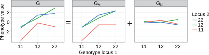
Figure 2. Decomposition of genotype-phenotye map into monotone and non-monotone components. Left panel: Genotype-phenotype map G for two loci underlying 10-week body-weight at 10 weeks in a mouse F2 cross. The GP map shown here is equivalent to the one in the original publication [see Figure 3A in Cheverud and Routman (1995)], but we have changed indexing of loci and alleles for consistency with the notation used here. The GP map G is decomposed with isotonic regression into a (middle panel) monotone component GM and a (right panel) non-monotone component GN.
For random GP maps (randomly sampled genotypic values as in (Gjuvsland et al., 2011)) there is a strong positive correlation between the degree of monotonicity and the size of the additive component (VA/VG) (Figure 3A). A similar relationship was observed for three-locus random GP maps (Figure A1A). All GP maps in Figure 3A with m < 0.1 have VA/VG < 0.1. At the other end of the spectrum there is much more variation, for instance the most extreme completely monotone map (the duplicate dominant factors DD) has VA/VG as low as 0.375.
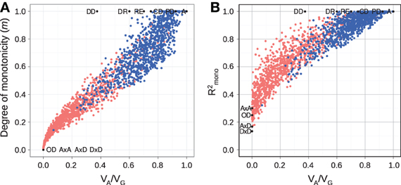
Figure 3. Measures of monotonicity vs. additivity of GP maps. Scatterplots showing VA/VG from unweighted regression vs. (A) degree of monotonicity (m) and (B) R2mono from isotonic regression. Black dots correspond to the maps shown in Figure 1 together with additive-by-dominance epistasis (A × D), a map with two loci showing complete dominance (CD) and two classical epistasis types from Table 1 in Phillips (1998); duplicate recessive genes (DR) and recessive epistasis (RE). Red dots show 1000 random two-locus GP maps, while blue dots show the same 1000 GP maps after rearranging genotypic values to introduce order-preservation for 1 locus [see Model and Methods in Gjuvsland et al. (2011)].
Measure 2: quantifying monotonicity by isotonic regression
This measure quantifies the monotonicity of a particular GP map G in terms of the least-squares distance to the closest monotone map. We build on the mathematical notation introduced in section “Background on monotonicity of GP maps” where Γ is the genotype space for N biallelic loci and a GP map is a function that assigns a real-valued genotypic value G(g) to each genotype g in Γ. For any particular GP map G, we identify the monotone component of G as the map GM which minimizes the residual variance var(G − GM), i.e., GM is the monotone GP map which is closest to G in the least-squares sense. For a given G the monotone component GM is unique (Barlow and Brunk, 1972) and can be computed numerically by isotonic regression (Leeuw et al., 2009) of G subject to the partial ordering of genotypes defined in Equation 1. Furthermore, the residual GN is orthogonal to GM in the sense that ∑g ∈ Γ GM (g)GN (g) = 0. This allows the orthogonal decomposition,
of a genotype-phenotype map into a monotone component GM and a non-monotone component GN such that var(G) = var(GM) + var(GN). The orthogonality property allows us to measure monotonicity of G in terms of the coefficient of determination R2mono of the isotonic regression given by the ratio R2mono = var(GM)/var(G). In the case that G itself is monotone for all loci we have R2mono = 1, while order-breaking for one or more loci will result in R2mono < 1.
The isotonic regression approach can be illustrated in a straightforward way on the two-locus GP map provided by Cheverud and Routman (1995) (see text above and left panel of Figure 2). The partial ordering of genotypes defined by Equation 1 is illustrated in Figure 1 (left panel). By isotone regression (Leeuw et al., 2009) on this partial genotype ordering, the original GP map is decomposed into a monotone and a non-monotone component (Figure 2, middle and right panels), and the coefficient of determination (R2mono) is 0.97.
Our simulation results for random GP maps show that R2mono is positively correlated to the size of the additive component (Figure 3B for two-locus GPs maps and Figure A1B for three-locus GP maps) and that for a given VA/VG the lower bound for R2mono is close to a straight line from (0, 0.2) to (1, 1). However, due to the search for the closest monotone GP map, R2mono will not become zero even for purely overdominant or purely epistatic maps. As shown in Figure A2, the two monotonicity measures are highly correlated.
An R package for studying monotonicity in GP maps
We developed an R package gpmap for studying functional properties of GP maps. The package takes GP maps in the form of vectors of genotypic values as input, and provides functions for (i) determining whether the map is order-breaking or order-preserving w.r.t. any given locus, (ii) the degree of monotonicity m, (iii) R2mono using isotonic regression from the isotone package (Leeuw et al., 2009), and (iv) plots of the original and decomposed GP maps. Code example 1 (Box 1) below illustrates the usage and functionality of the gpmap package. The package is available from CRAN http://cran.r-project.org/package=gpmap under GPLv3.

Box 1. Code example 1.
Monotonicity in GP Maps Arising from Gene Regulatory Networks
To search for generic relationships between monotonicity and regulatory network structure, we used the above measures of monotonicity to characterize GP maps emerging from the gene regulatory network models (see Models and Methods). Based on earlier results (Gjuvsland et al., 2007, 2011; Wang et al., 2013) we hypothesized that incoherent feed forward (Figure 4, right panel) or positive feedback (Figure 4, left panel) would be necessary in order to obtain highly order-breaking GP maps, and we characterized all 1881 networks in terms of these two properties. Table 1 shows the number of motifs falling into the resulting four categories. We summarized the number of Monte Carlo simulations where all genotypic parameter sets gave convergence to a stable steady state, and where the resulting GP maps were not essentially flat (see Models and Methods for details). Motifs with less than 100 usable GP maps were discarded from further analysis. For the genotype-to-parameter maps without pleiotropy (in the sense that genetic variation at one locus influences only a single parameter, see Model and Methods) 868 motifs were discarded, while for the genotype-to-parameter map with pleiotropy (genetic variation at one locus influences three parameters) 791 motifs were discarded. All (but one) discarded motifs contained at least one positive feedback loop (Table 1). A plausible explanation for this is that many motifs with positive feedback loops have a stable steady state at, or very close to 0 for one or more state variables regardless of parameter values, and this leads to essentially flat GP maps.
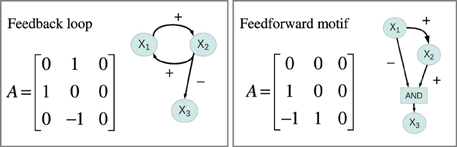
Figure 4. Connectivity matrices and signed directed graphs. Connectivity matrix A and the corresponding signed directed graph for two of the 1881 systems in the simulation study. The left panel depicts the connectivity matrix and the signed digraph of a system with a positive feedback loop between X1 and X2 while the right panel shows a system with incoherent feedforward from X1 to X3.
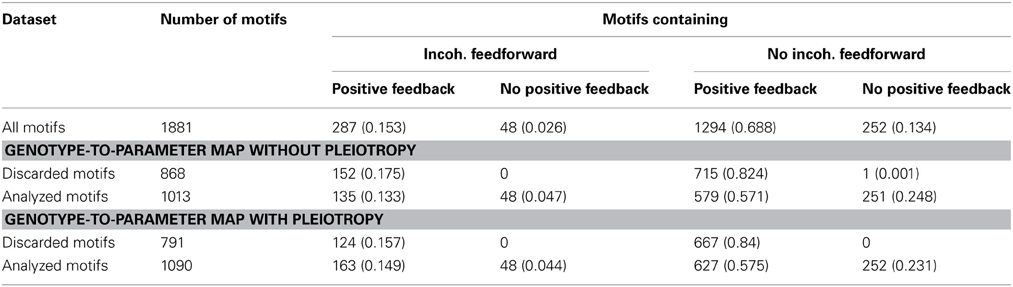
Table 1. Frequencies (proportion of row total in parenthesis) of incoherent feedforward and positive feedback loops in subsets of the 1881 studied motifs.
The introduction of pleiotropy in the genotype to parameter map has a marked effect on the monotonicity characteristics of the associated GP map (Figure 5). When genetic variation at a locus Xi affects only its maximal production rate the GP maps come out as highly monotone (Figure 5A), with a large majority being fully monotone or order-breaking for just a single locus. When genetic variation at locus Xi affects the threshold and steepness of the dose-response curve in addition to the maximal production rate (pleiotropy in the genotype-to-parameter map), the majority of GP maps still show order-breaking either for no loci or just one locus (Figure 5B). But a considerable number of GP maps are in this case order-breaking for two or three loci. Furthermore, by dividing the motifs into the four groups given in Table 1 it is evident that the regulatory anatomy of a network determines its predisposition for non-monotonicity in its associated GP map. Presence of incoherent feedforward or positive feedback loops appears to be prerequisites for the majority of the observed non-monotonic GP maps.
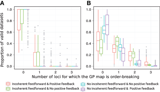
Figure 5. Order-breaking in motifs containing a single feedforward loop. Summary of order-breaking for all motifs for which at least 100 (out of 1000) Monte Carlo simulations lead to GP maps with non-negligible variation (see Models and Methods section “Gene regulatory network simulations,” for detailed criteria). Results are shown for 1013 motifs with a genotype-to-parameter map without pleiotropy (A) and 1090 motifs with a genotype-to-parameter map with pleiotropy (B). Colors indicate classes of motifs based on the presence/absence of incoherent feedforward and positive feedback loops, see Table 1 for the number of motifs in each class. A single boxplot summarizes, for all motifs in the given class, the proportion of the GP maps (y-axis) that are order-breaking with respect to a given number of loci (x-axis). For example, consider the red box at x = 0 in panel (A). This boxplot contains results for motifs with both incoherent feedforward and positive feedback and from Table 1 we find that the red boxplot summarizes results for 135 motifs. From the y-axis we find that at least half (box median at y = 1) of these 135 motifs result in only monotone GP maps, while for the most extreme (end of whisker) of the 135 motifs only 25% of the GP maps are monotone. Similarly, the cyan box is compressed into a line at x = 0, y = 1 indicating that all 251 motifs that lack both incoherent feedforward and positive feedback result in only monotone GP maps.
The class of motifs lacking both incoherent feedforward and positive feedback contains very few order-breaking GP maps, and with no pleiotropy in the genotype-to-parameter map we observe only fully order-preserving GP maps for this class (cyan in Figure 5A). In the Appendix we generalize this to an arbitrary number of nodes and formally prove that without pleiotropy in the genotype-to-parameter map, the presence of incoherent feedforward or positive feedback is indeed a necessary condition for non-monotone GP maps to arise from networks with monotone gene regulation functions.
The introduction of pleiotropy in the genotype-to-parameter map increases the frequency of order-breaking GP maps substantially (Figure 5B). Motifs lacking both incoherent feedforward and positive feedback may in this case lead to GP maps that are order-breaking for one or two loci, but never for all three loci. Using isotonic regression to quantify the overall monotonicity of the GP maps reinforces the finding that incoherent feedforward and positive feedback predispose for non-monotonicity (Figure 6). Figure 6 also shows that for all classes of motifs the majority of GP maps are fully monotone, while the most non-monotone GP maps (lowest R2mono values) are observed for motifs with positive feedback. The differences between classes of motifs are also evident when inspecting the additivity of GP maps (Figure A3), but since monotone GP maps can still be non-additive, the patterns are much more blurred than for monotonicity.
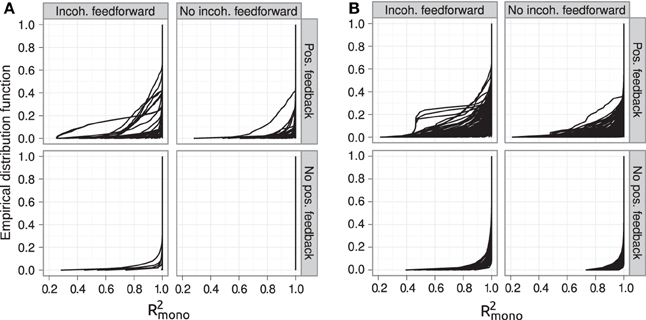
Figure 6. Empirical distribution functions for R2mono. Summary of R2mono values from isotone regression for all motifs for which at least 100 (out of 1000) Monte Carlo simulations lead to GP maps with non-negligible phenotypic variation (see Models and Methods section “Gene regulatory network simulations,” for detailed criteria). Results are shown for 1013 motifs with a genotype-to-parameter map without pleiotropy (A) and 1090 motifs with a genotype-to-parameter map with pleiotropy (B). Each panel is divided into 4 subplots containing classes of motifs based on the presence/absence of incoherent feedforward and positive feedback loops, see Table 1 for the number of motifs in each class. Each curve shows, for a single motif, the empirical distribution function value (y-axis) of R2mono for all GP maps (x-axis).
Discussion
Fisher's (1918) regression on gene content and the concepts derived from this, such as additive effects and dominance deviation, provide the theoretical basis for most of quantitative genetics (Falconer and Mackay, 1996; Lynch and Walsh, 1998). By regressing on gene content, including the extensions by Cockerham (1954), the genotype-phenotype map is decomposed into additive, dominant, and epistatic components. The use of gene content or the number (0, 1, or 2) of alleles with a particular index in a genotype implies the same partial ordering of genotype space as defined in Equation 1. Thus, our proposed definition of monotonicity of GP maps, and in particular the use of isotonic regression to quantify monotonicity, may be viewed as a relaxation of the linearity assumption underlying current quantitative genetics theory. In this perspective the positive correlation between monotonicity and additivity (Figure 3) is expected.
We have addressed GP maps with 2 and 3 loci as we considered an in-depth study of the properties of GP maps with higher number of loci to be outside the scope of this study. Some general observations can be made, though. Since m is a weighted average, the mk of major loci (i.e., for which Tk is large relative to ∑ Tk) will tend to dominate. For instance, in a case with a single major locus showing monotone gene action and several minor loci showing order-breaking, the GP map will overall be close to monotone (m close to 1). Conversely, order-preservation in a number of minor loci would have little influence on m if major loci have strongly non-monotone gene action. Isotonic regression gives an overall measure of monotonicity of a GP map, but provides no locus-specific measures corresponding to mk. Similar to the case for m, the gene action of major loci will have high influence on the value of R2mono.
The observation that monotonicity is an important property of GP maps is in principle not new. For a single locus, non-monotone gene action appears in the form of over- or under-dominance, while complete and partial dominance as well as additivity exemplify monotone gene action. Weinreich et al. (2005) distinguished between sign epistasis and magnitude epistasis and showed that sign epistasis limits the number of mutational trajectories to higher fitness. As sign epistasis reflects a non-monotone GP relationship and magnitude epistasis reflects a monotone one, this insight concords with our results. A similar distinction has been proposed (Wang et al., 2010) for statistical interactions where removable interactions are those that can be removed by a monotone transformation of the phenotype scale, while non-monotonicity in the GP map leads to essential interactions. Wu et al. (2009) developed a method to screen for and test the significance of essential interaction in genome-wide association studies. Isotonic regression has also recently been applied to link genotype and phenotype data (Beerenwinkel et al., 2011; Luss et al., 2012). Our treatment of monotonicity is more general than these earlier works in three major ways. First, we deal with monotonicity of the GP map as a whole rather than either intra-locus (dominance vs. overdominance) or inter-locus (magnitude vs. sign epistasis and removable vs. essential interactions). Second, where the earlier treatments have focused on classifying the type of gene action, we make use of quantitative measures of monotonicity. Third, our approach combining the concept of monotonicity with cGP models opens a direct link between genetics and the theory of dynamical systems in the wide sense.
Monotonicity is a property of the GP map separate from the allele frequencies, making it a physiological (Cheverud and Routman, 1995) or functional (Hansen and Wagner, 2001) descriptor rather than a statistical one. The distinction between physiological and statistical epistasis has lead to much debate (Phillips, 2008). Zeng et al. (2005) argued the distinction was unnecessary and potentially misleading. Although their arguments around orthogonality and variance components are valid, our results demonstrate very clearly that describing the properties of the GP map without reference to any particular study population is essential if we want to connect quantitative genetics with regulatory biology.
It is clear from our results that positive feedback and incoherent feedforward promote non-monotonicity. The clear-cut differences in monotonicity between different classes of regulatory networks, combined with the strong correlation between monotonicity and additivity of GP maps, appear therefore to explain the findings that regulatory systems with positive feedback give considerably more statistical epistasis than those without (Gjuvsland et al., 2007; Wang et al., 2013). Even though both incoherent feedforward and positive feedback predispose for non-monotone GP maps, the underlying mechanisms are different for the two regulatory motifs. In the case of incoherent feedforward the sum of direct and indirect effects may result in a non-monotone dose-response relationship (Kaplan et al., 2008). That positive feedback loops can give non-monotonicity is intuitively less clear, but in the Appendix we show both results analytically. Positive feedback predisposes for multiple steady states, and order-breaking might also emerge from different genotypes corresponding to different states. It should be noted, however that positive feedback is only a necessary condition for multistationarity (Plahte et al., 1995), and a positive loop in the connectivity matrix A of a system is not necessarily active at any point during the time course of the system.
Without any restrictions on the connectivity of a three-gene system there are 39 = 19, 683 possible distinct networks. The main restriction we imposed (see Models and Methods for details) was a maximum of two regulators per gene, which allowed us to use Boolean gene regulation functions already established in the sigmoid formalism (Plahte et al., 1998). Other model formalisms allowing an arbitrary number of regulators are also available (Wagner, 1994, 1996; Siegal and Bergman, 2002) and could be extended to diploid forms and used in later studies.
Although this study has focused on gene regulatory networks, the concept of monotone gene action applies to the propagation of genetic variation across the whole physiological hierarchy. One may therefore systematically use the concepts and methods presented here to study the order-preserving and order-breaking properties of genotype-phenotype mappings that are associated with any regulatory structure amenable for mathematical modeling. Through this it will be possible to make a wide-ranging survey of which regulatory anatomies promote monotonicity and which promote non-monotonicity. We foresee that this classification may become instrumental for predicting how phenotypic effects of genetic variation propagate across generations in sexually reproducing populations.
Conflict of Interest Statement
The authors declare that the research was conducted in the absence of any commercial or financial relationships that could be construed as a potential conflict of interest.
Supplementary Material
The Supplementary Material for this article can be found online at: http://www.frontiersin.org/journal/10.3389/fgene.2013.00216/abstract
Spreadsheet S1 | Excel spreadsheet with connectivity matrices and loop products for all 1881 gene regulatory networks.
References
Alon, U. (2007). Network motifs: theory and experimental approaches. Nat. Rev. Genet. 8, 450–461. doi: 10.1038/nrg2102
Alvarez-Castro, J. M., and Carlborg, Ö. (2007). A unified model for functional and statistical epistasis and its application in QTL analysis. Genetics 176, 1151–1167. doi: 10.1534/genetics.106.067348
Barlow, R. E., and Brunk, H. D. (1972). The isotonic regression problem and its dual. J. the Am. Stat. Assoc. 67, 140–147. doi: 10.1080/01621459.1972.10481216
Beerenwinkel, N., Knupfer, P., and Tresch, A. (2011). Learning monotonic genotype-phenotype maps. Stat. Appl. Genet. Mol. Biol. 10:3. doi: 10.2202/1544-6115.1603
Cheverud, J. M., and Routman, E. J. (1995). Epistasis and its contribution to genetic variance components. Genetics 139, 1455–1461.
Cheverud, J. M., and Routman, E. J. (1996). Epistasis as a source of increased additive genetic variance at population bottlenecks. Evolution 50, 1042–1051. doi: 10.2307/2410645
Cockerham, C. C. (1954). An extension of the concept of partitioning hereditary variances for analysis of covariances among relatives when epistasis is present. Genetics 39, 859–882.
De Jong, H. (2002). Modeling and simulation of genetic regulatory systems: a literature review. J. Comput. Biol. 9, 67–103. doi: 10.1089/10665270252833208
Falconer, D. S., and Mackay, T. F. C. (1996). Introduction to Quantitative Genetics. Harlow: Longman Group.
Fisher, R. A. (1918). The correlation between relatives on the supposition of Mendelian inheritance. Trans. R. Soc. Edinb. 52, 399–433. doi: 10.1017/S0080456800012163
Gjuvsland, A. B., Hayes, B. J., Omholt, S. W., and Carlborg, Ö. (2007). Statistical epistasis is a generic feature of gene regulatory networks. Genetics 175, 411–420. doi: 10.1534/genetics.106.058859
Gjuvsland, A. B., Vik, J. O., Beard, D. A., Hunter, P. J., and Omholt, S. W. (2013). Bridging the genotype-phenotype gap: what does it take? J. Physiol. 591, 2055–2066. doi: 10.1113/jphysiol.2012.248864
Gjuvsland, A. B., Vik, J. O., Woolliams, J. A., and Omholt, S. W. (2011). Order-preserving principles underlying genotype-phenotype maps ensure high additive proportions of genetic variance. J. Evol. Biol. 24, 2269–2279. doi: 10.1111/j.1420-9101.2011.02358.x
Hansen, T. F., and Wagner, G. P. (2001). Modeling genetic architecture: a multilinear theory of gene interaction. Theor. Popul. Biol. 59, 61–86. doi: 10.1006/tpbi.2000.1508
Hill, W. G., Goddard, M. E., and Visscher, P. M. (2008). Data and theory point to mainly additive genetic variance for complex traits. PLoS Genet. 4:e1000008. doi: 10.1371/journal.pgen.1000008
Jaeger, J., Irons, D., and Monk, N. (2012). The inheritance of process: a dynamical systems approach. J. Exp. Zool. B Mol. Dev. Evol. 318, 591–612. doi: 10.1002/jez.b.22468
Kaplan, S., Bren, A., Dekel, E., and Alon, U. (2008). The incoherent feed-forward loop can generate non-monotonic input functions for genes. Mol. Syst. Biol. 4, 203. doi: 10.1038/msb.2008.43
Karlebach, G., and Shamir, R. (2008). Modelling and analysis of gene regulatory networks. Nat. Rev. Mol. Cell Biol. 9, 770–780. doi: 10.1038/nrm2503
Le Rouzic, A., and Alvarez-Castro, J. M. (2008). Estimation of genetic effects and genotype-phenotype maps. Evol. Bioinformatics 4, 225–235. doi: 10.4137/EBO.S756. Available online at: http://www.la-press.com/estimation-of-genetic-effects-and-genotype-phenotype-maps-article-a887
Leeuw, J. D., Hornik, K., and Mair, P. (2009). Isotone optimization in R: pool-adjacent-violators algorithm (PAVA) and active set methods. J. Stat. Softw. 32, 1–24.
Luss, R., Rosset, S., and Shahar, M. (2012). Efficient regularized isotonic regression with application to gene–gene interaction search. Ann. Appl. Stat. 6, 253–283. doi: 10.1214/11-AOAS504
Lynch, M., and Walsh, B. (1998). Genetics and Analysis of Quantitative Traits. Sunderland, MA: Sinauer Associates.
Mestl, T., Plahte, E., and Omholt, S. W. (1995). A mathematical framework for describing and analysing gene regulatory networks. J. Theor. Biol. 176, 291–300. doi: 10.1006/jtbi.1995.0199
Moore, A. (2012). Towards the new evolutionary synthesis: gene regulatory networks as information integrators. Bioessays 34, 87–87. doi: 10.1002/bies.201290000
Neale, B. M., Ferreira, M. A. R., Medland, S. E., and Posthuma, D. (eds.). (2008). Statistical Genetics: Gene Mapping through Linkage and Association. New York, NY: Taylor and Francis Group.
Omholt, S. W., Plahte, E., Øyehaug, L., and Xiang, K. F. (2000). Gene regulatory networks generating the phenomena of additivity, dominance and epistasis. Genetics 155, 969–980.
Phillips, P. C. (2008). Epistasis - the essential role of gene interactions in the structure and evolution of genetic systems. Nat. Rev. Genet. 9, 855–867. doi: 10.1038/nrg2452
Plahte, E., Mestl, T., and Omholt, S. W. (1995). Feedback loops, stability and multistationarity in dynamical systems. J. Biol. Syst. 3, 409–413. doi: 10.1142/S0218339095000381
Plahte, E., Mestl, T., and Omholt, S. W. (1998). A methodological basis for description and analysis of systems with complex switch-like interactions. J. Math. Biol. 36, 321–348. doi: 10.1007/s002850050103
Schlitt, T., and Brazma, A. (2007). Current approaches to gene regulatory network modelling. BMC Bioinformatics 8(Suppl. 6):S9. doi: 10.1186/1471-2105-8-S6-S9
Siegal, M. L., and Bergman, A. (2002). Waddington's canalization revisited: developmental stability and evolution. Proc. Natl. Acad. Sci. U.S.A. 99, 10528–10532. doi: 10.1073/pnas.102303999
Wagner, A. (1994). Evolution of gene networks by gene duplications: a mathematical model and its implications on genome organization. Proc. Natl. Acad. Sci. U.S.A. 91, 4387–4391. doi: 10.1073/pnas.91.10.4387
Wagner, A. (1996). Does evolutionary plasticity evolve? Evolution 50, 1008–1023. doi: 10.2307/2410642
Wang, X., Elston, R. C., and Zhu, X. (2010). The meaning of interaction. Hum. Hered. 70, 269–277. doi: 10.1159/000321967
Wang, Y., Vik, J. O., Omholt, S. W., and Gjuvsland, A. B. (2013). Effect of regulatory architecture on broad versus narrow sense heritability. PLoS Comput. Biol. 9:e1003053. doi: 10.1371/journal.pcbi.1003053
Weinreich, D. M., Watson, R. A., and Chao, L. (2005). Perspective: sign epistasis and genetic constraint on evolutionary trajectories. Evolution 59, 1165–1174. doi: 10.1554/04-272
Wu, C., Zhang, H., Liu, X., Dewan, A., Dubrow, R., Ying, Z., et al. (2009). Detecting essential and removable interactions in genome-wide association studies. Stat. Interface 2, 161–170. doi: 10.4310/SII.2009.v2.n2.a6
Zeng, Z. B., Wang, T., and Zou, W. (2005). Modeling quantitative trait loci and interpretation of models. Genetics 169, 1711–1725. doi: 10.1534/genetics.104.035857
Appendix
In this appendix we complement the simulation studies in the main text with some analytic results for GP maps emerging from ODE models of gene regulatory networks. We study a generalization of the gene network model in Equation (3) with an arbitrary number of loci and monotone gene regulation functions, but restrict the analysis to genotype-parameter maps without pleiotropy. In particular, we show that (i) if there are no positive feedback loops and no incoherent feedforward loops in the network, the resulting GP maps are always monotone, (ii) a positive feedback loop or an incoherent feedforward loop may lead to non-monotone GP maps. The results hold for phenotypes given as the stable concentration of the product of one of the genes, and under certain restrictions also for phenotypes given as a function of one or several stable gene product concentrations that is monotonic with respect to each of its arguments.
Gene Network Model
We consider a dynamic system consisting of n mutually interacting diploid loci Xj, j ∈ N = {1, …, n}, regulating each other's expression. The time dependent output of Xj is denoted zj, and we define z = [z1, z2, …, zn]. It goes without saying that zj in general depends on the genotypes of all the genes even though we will not always state this explicitly.
For a given genotype g = gjg(j) = ajbjg(j), where gj ∈ {11, 12, 22} denotes the genotype and aj, bj ∈ 1, 2 denote the indexes of the two alleles of locus Xj, the equations of motion for Xj are
where z1j and z2j are the time-dependent outputs of the two homologous copies of Xj. The two allele rate functions r1j(z) and r2j(z) have range [0, 1] so that α1j and α2j represent the maximum production rates of the two alleles. We assume that all dose-response functions in Equation (A1) are differentiable and monotonic with respect to each of its arguments, and that for each j, k, the signs of ∂r1j/∂xk and ∂r2j/∂xk in the stable point x are equal. This model generalizes Eq. (3) to an arbitrary number of loci and a broader class of gene regulation functions.
In the following we are only concerned with the steady states of Equation (A1), and assume for simplicity that they have just a single stable equilibrium point. Solving the equilibrium conditions of Equation (A1) with respect to z1j and z2j and adding gives
where x = [x1, …, xn] is the stable point, μaij = αajj/γajj and μbjj = αbjj/γbjj. Since our definition of monotonicity of GP maps does not depend on the numbering of alleles, we will without loss of generality assume μ1j ≤ μ2j for all j.
The network architecture can be read out from the structure of the system's Jacobian matrix in the stable state x. We define the elements of the Jacobian J for the set of functions fj defined in Equation (A2) by
To the Jacobian J it is customary to assign a signed directed graph  in which each locus Xk is represented by a node Xk, and in which there is an arc from Xj to Xk if and only if Jkj ≠ 0, its sign given by the sign of Jkj. A chain from Xj to Xk is a set of arcs in leading from Xj to Xk in which all intermediate nodes are visited only once. The sign of a chain is equal to the product of the signs of the Jij corresponding to the arcs in the chain. If there is a chain from Xi to Xj and also a chain from Xj to Xi through a disjoint set of nodes, the two chains constitute a proper feedback loop (FBL). To each FBL is associated a loop product L which is the product of the Jacobian elements corresponding to all the arcs in the loop. The sign of the loop is given by the sign of L. Two chains from Xj to Xi, i ≠ j, with only the endpoint nodes in common, constitute a feedforward loop (FFL). If the two chains have opposite signs, the FFL is incoherent (IFFL), otherwise it is coherent (CFFL).
The system's phenotype could be any scalar quantity defined by its equilibrium value x. In the following we assume the genotype-phenotype map G(g) = xq(g), q ∈ N, for a given and fixed q, and investigate the monotonicity properties of G(gkg(k)) with respect to genetic variation in any locus Xk for different backgrounds g(k). In the following sections we analyse the causes of order-breaking in G in the restricted case in which there is only genetic variation in μ1k and μ2k, not in the shape of the dose-response functions r1k and r2k, implying r1k(x) = r2k(x) = rk(x). This is what we mean by a genotype-to-parameter map without pleoitropy.
In the next sections we prove the following result:
Proposition 1. Assume all rate functions in Equation (A1) are monotonic and that G is the mapping from g to xq for some fixed q so that xq(g) is the phenotype. If there is no feedback loop (FBL) and no feedforward loop (FFL) anywhere in the network corresponding to the system Equation (A1), then necessarily mk = 1 for all k. If the system contains either a single FFL or a single FBL, then G may be non-monotone for some xk if the FFL is positive or the FBL is incoherent, but if the FBL is negative or the FFL is coherent, no order breaking can occur for any xk.
At the end of this note we show that under some reasonable conditions this result is also valid for more general phenotypes depending on more than one xq.
Networks Without Loops
We first consider networks containing no feedforward loop and no feedback loop. In these networks there is at most one chain from one node to another, and of course no autoregulatory loops. If there is a chain from Xj to Xk, there is no chain from Xk to Xj. Any node is either unregulated (constitutively expressed) or regulated by one or several other nodes.
We first prove a useful lemma.
Lemma 1. If xl(11g(j)) ≤ xl(12g(j)) ≤ xl(22g(j)) for any j and l and there is an arc Xl → Xm with positive sign and no other chain from Xl → Xm, then also xm(11g(j)) ≤ xm(12g(j)) ≤ xm(22g(j)). If the sign of the arc is negative, then xm(11g(j)) ≥ xm(12g(j)) ≥ xm(22g(j)).
Proof. Suppressing the explicit dependence on other genes that are not affected by genetic variation in Xj, we have
Now, rm is monotonic by assumption. If it is monotonically increasing,
from which the assertion follows. If rm is monotonically decreasing, we find the same relations with the inequality signs reversed. □
If there is no chain from Xj to Xq, genetic variation in Xj will not be reflected in G, i.e. G(11g(j)) = G(12g(j)) = G(22g(j)), and by definition does not give order-breaking. Then assume Xj is upstream relative to Xq and that the chain from Xj to Xq is positive. We first let Xj be an unregulated node with no predecessor. Then
because r1j = r2j = 1. From this it follows that xj(11g(j)) ≤ xj(12g(j)) ≤ xj(22g(j)).
Repeated use of Lemma 1 leads eventually to xq(11g(j)) ≤ xq(12g(j)) ≤ xq(22g(j)), irrespective of the genotypic background of Xj. If the chain from Xj to Xq is negative, the argument goes in the same way, but then xq(11g(j)) ≥ xq(12g(j)) ≥ xq(22g(j)). The above argument can be carried out in the same way if Xj is not top-stream. It follows that in a network without FFBs and FFLs and where genetic variation is restricted to μ1k and μ2k, the genotype-phenotype map G(g) = xq(g) cannot be order-breaking.
Networks with a Feedback Loop
In this section we investigate the effects of feedback loops on the degree of monotonicity. Assuming monotonic dose-response functions and non-pleiotropic genetic variation, we show that a positive feedback loop may lead to order breaking, while negative feedback loops never do. We consider a network in which there is no FFL and a single FBL with Xq as one of its members and Xk is upstream of the loop.
Lemma 2. Consider a network with n nodes for which all dose-response functions are monotonic and there is only genetic variation in μ1k and μ2k. Asssume there is a chain from Xk to X1, that X1, but not Xk, is member of a FBL with m nodes, and that there is no other FBL and no FFL in the system. If Xq is in the loop, let the loop be X1 → X2 → … → Xq → … → Xm → X1. If the FBL is positive, there may be order-breaking in Xq due to genetic variation in Xk, but no order-breaking can occur if the loop is negative. If Xq is downstream of the loop, the same result applies.
Proof. With a single FBL and no FFL there is at most one directed path from any node Xi to any other node Xj, and if there is a path from Xi to Xj, there is no return path from Xj to Xi if either Xi or Xj is not part of the FBL. We first consider the dependence of x1 on xk. The direct regulators of node X1 are Xm and Xl, the latter being the last but one node in the chain from Xk to X1. In Plahte et al. (2013) we introduced the propagation functions xj = pjk(xk) which express the effect on xj of genetic variation in Xk. An important property of pjk is that it can be derived from all the equilibrium conditions Equation (A2) except the equation for fk. This implies that the effects on Xj of genotypic variation in Xk are only expressed in terms of the variations in xk, while the parameters expressing the genotype of Xk do not enter into the function pjk.
We then have xl = plk(xk) and xm = pm1(x1). To make it easier to use the results in Plahte et al. (2013) we rewrite the equilibrium condition Equation (A2) as
where γj > 0. In the following, the Jacobian refers to this set of equations, which has the same root and the same functional dependencies between the variables as the original set. The signs of the partial derivatives of Rj are the same as for rajj and rbjj. The equilibrium condition for X1 is then
This equation defines x1 as a function of xk in an open domain around the equilibrium point and with a derivative that can be computed by implicit differentiation, i.e.
where qij = p′ij is the derivative of pij for all i, j.
From Lemma 1 it follows that there is no order breaking in Xl, in other words, qlk has a fixed sign. Consider then qm1. There is just a single chain from X1 to Xm, and Equation (13) in Plahte et al. (2013) gives
Here U is the set of nodes in this chain, CU is its chain product, i.e. the product of the Jacobian elements corresponding to the arcs in the chain, V = N \ U, D(11) is the subdeterminant of J with row 1 and column 1 deleted, and DVV is the subdeterminant of J composed of the rows and columns V. Because there is no feedback loop among the nodes represented in D(11) and DVV, only the diagonal degradation terms contribute to these two determinants. Hence D(11) = (−1)n − 1 ∏i ≠ 1 γi. Similarly, DVV = (−1)n − m ∏i ∈ V γi, giving qml = γ1CU/ΓU, where ΓU = ∏i ∈ U γi. Finally, we note that P = (∂ R1/∂ xm)CU is the loop product of the loop.
Solving Equation (A9) with respect to dx1/dxk and using all these expressions lead to
The sign of ∂x1/∂xl is independent of the genotype of Xk and the sign of q1k is fixed. Genotypic variation in Xk may change the magnitude of P, but its sign is fixed because all Jacobi elements have fixed sign independent of the system parameters. Thus, genotypic variation in Xk does not alter the sign of dx1/dxk if the loop is negative (P < 0), while for a positive loop the sign of ΓU − P may switch. In the latter case, an increase in xk due to genetic variation in Xk may increase x1 in some cases and decrease it in others, leading to order breaking. As there is only a single chain from X1 to Xq, no order breaking in X1 implies no order breaking in Xq, while order breaking in X1 may propagate to Xq. The same result follows if Xq is downstream a node in the loop because order breaking in this node may propagate to Xq. □
Feedforward Loops (FFLs)
A feedforward loop (FFL) is a motif in the network in which there are two different chains C1 and C2 from one particular node to another particular node. To each chain Ci is associated a chain product Pi defined as the product of the Jacobian elements corresponding to the arcs in Ci. If P1 and P2 have equal signs, the FFL is coherent, otherwise it is incoherent.
In a network with a single feedforward loop and no feedback loops we now investigate the effect on G(g) = xq(xk(g)) of genetic variation in Xk for varying background g(k). Our starting point is again Equation (A7). We first let Xk and Xq be the initial and terminal nodes in the FFL. The two chains C1 and C2 leading from Xk to Xq comprise ρ1 and ρ2 nodes including Xk and Xq, respectively. Let the set of nodes in C1 and C2 be XU1 and XU2, respectively, where U1 and U2 are the corresponding subsets of N, and let V1 and V2 be their complements.
Roughly speaking, the derivative of the propagation function pqk(xk) can be expressed as a sum of terms, each term corresponding to one of the chains leading from Xk to Xq (Plahte et al., 2013). To the chain Ci is assigned the chain weight wi given by
where DViVi is the Jacobian subdeterminant for the nodes not included in Ci, and D(kk) is the Jacobian subdeterminant for all nodes except Xk. Because there are two chains from Xk to Xq, the derivative of pqk is a sum of two terms:
where P1 and P2 are the two chain products, and w1 and w2 their weights (Plahte et al., 2013). When there is no feedback loop in the system, only the diagonal elements in J stemming from the term −γi xi in Equation (A7) contribute to the determinants DViVi and D(kk):
Altogether this gives
where Γ1 and Γ2 are the products of the γj in the two chains, respectively. The chain products P1 and P2 depend on the genotype gk of Xk as well as on the genotypic background g(k), but their signs S1 and S2 are invariant under genotypic variation. It is easy to see that a negative autoregulatory loop, which is a common feature in gene regulatory networks, would not invalidate the conclusion, but a positive autoregulatory loop might.
If the FFL is incoherent, P1 and P2 have opposite signs, implying that the sign of dxq/dxk may vary. If the FFL is coherent, however, no order-breaking can occur.
If Xk is upstream relative to the initial node Xinit of the FFL, it follows from the above section on networks without loops that there will be no order-breaking in Xinit, and the above argument is still valid.
More General Phenotypes
In real life, relevant phenotypes are not direct gene products, but rather functions of the concentrations of one or several gene products. Let the phenotype G(g) be a function of xU(g), G = h(xU(g)), where U is a subset of N, and assume that for any u ∈ U, ∂h/∂xu has fixed sign for all genotypes. To analyse this case we extend the original system Equation (A2) to
and apply our above results to this system, in which G(g) = xn + 1(g), i.e. q = n + 1. If there are two nodes among XU which have a common predecessor Xk, then there will exist two chains from Xk to Xn + 1. These two chains constitute a feedforward loop with Xn + 1 as final node. If this FFL is incoherent, order breaking due to genetic variation in Xk may occur even if there is no order breaking in the original system comprising the nodes X1, …, Xn. If the FFL is coherent, order breaking only occurs if it occurs in the original system.
References
Plahte, E., Gjuvsland, A. B., and Omholt, S. W. (2013). Propagation of genetic variation in gene regulatory networks. Phys. D 256–257, 7–20. doi: 10.1016/j.physd.2013.04.002
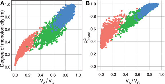
Figure A1. Measures of monotonicity vs. additivity of GP maps with three loci. Scatterplots showing VA/VG from unweighted regression vs. (A) degree of monotonicity (m) and (B) R2mono. Red dots show 1000 random three-locus GP maps, blue dots show the same 1000 GP maps after sorting to introduce order-preservation for 1 locus while green dots show the same 1000 GP maps after sorting to introduce order-preservation for 2 loci [see Model and Methods in Gjuvsland et al. (2011)].
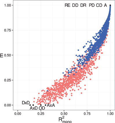
Figure A2. Comparing measures of monotonicity GP maps. Scatterplots showing degree of monotonicity (m) vs. R2mono. Black dots correspond to the maps shown in Figure 1. Red dots show 1000 random two-locus GP maps, while blue dots show the same 1000 GP maps after sorting to introduce order-preservation for 1 locus [see Model and Methods in Gjuvsland et al. (2011)].
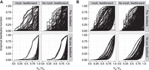
Figure A3. Empirical distribution functions for additivity of GP maps. Summary of VA/VG from unweighted regression for all motifs for which at least 100 (out of 1000) Monte Carlo simulations lead to GP maps with non-negligible phenotypic variation (see Models and Methods section “Gene regulatory network simulations,” for detailed criteria). Results are shown for 1013 motifs with a genotype-to-parameter map without pleiotropy (A) and1090 motifs with a genotype-to-parameter map with pleiotropy (B). Each panel is divided into 4 subplots containing classes of motifs based on the presence/absence of incoherent feedforward and positive feedback loops, see Table 1 for the number of motifs in each class. Each curve shows, for a single motif, the empirical distribution function value (y-axis) of VA/VG from unweighted regression for all GP maps (x-axis).
Keywords: genotype-phenotype map, gene regulatory networks, epistasis, variance component analysis, genetic modeling, systems genetics, genetic variance, monotonicity
Citation: Gjuvsland AB, Wang Y, Plahte E and Omholt SW (2013) Monotonicity is a key feature of genotype-phenotype maps. Front. Genet. 4:216. doi: 10.3389/fgene.2013.00216
Received: 17 June 2013; Accepted: 07 October 2013;
Published online: 07 November 2013.
Edited by:
José M. Álvarez-Castro, Universidade de Santiago de Compostela, SpainReviewed by:
Arnaud Le Rouzic, Centre National de la Recherche Scientifique, FranceOvidiu Dan Iancu, Oregon Health & Science University, USA
Copyright © 2013 Gjuvsland, Wang, Plahte and Omholt. This is an open-access article distributed under the terms of the Creative Commons Attribution License (CC BY). The use, distribution or reproduction in other forums is permitted, provided the original author(s) or licensor are credited and that the original publication in this journal is cited, in accordance with accepted academic practice. No use, distribution or reproduction is permitted which does not comply with these terms.
*Correspondence: Arne B. Gjuvsland, Centre for Integrative Genetics (CIGENE), Department of Mathematical Sciences and Technology, Norwegian University of Life Sciences, PO Box 5003, N-1432 Ås, Norway e-mail: arne.gjuvsland@umb.no