Improved Motion Description for Action Classification

1. Introduction

The recognition of human actions in unconstrained videos remains a challenging problem in computer vision despite the fact that human actions are often attributed to essential meaningful content in such videos. The field receives sustained attention due to its potential applications, such as for designing video-surveillance systems, in providing automatic annotation of video archives, as well as for improving human–computer interaction. The solutions that were proposed to address the above problems were inherited from the techniques first designed for image search and classification.

Successful local features were developed to describe image patches (Schmid and Mohr, 1997; Lowe, 2004) and translated in the 2D + t domain as spatio-temporal local descriptors (Laptev et al., 2008; Wang et al., 2009) and now include motion clues of Wang et al. (2011). These descriptors are often extracted from spatial–temporal interest points (Laptev and Lindeberg, 2003; Willems et al., 2008). Furthermore, several approaches assume underlying temporal motion model involving trajectories (Hervieu et al., 2008; Matikainen et al., 2009; Messing et al., 2009; Sun et al., 2009; Brox and Malik, 2010; Wang et al., 2011; Wu et al., 2011; Gaidon et al., 2012; Wang and Schmid, 2013).

Most of the above-mentioned methods produce a large set of local descriptors, which are in turn aggregated into a single vector representing the video. These enable the use of powerful discriminative classifiers such as support vector machines (SVMs). This is usually done with the bag-of-words technique (Sivic and Zisserman, 2003) that quantizes local features with a k-means codebook. Thanks to the successful combination of this encoding technique, the state-of-the-art in action recognition is able to go beyond the toy problems of simple human action classification in controlled environments and is able to consider actions detection in video clips and movies (Marzalek et al., 2009; Kuehne et al., 2011; Soomro et al., 2012). Even though the subject has witnessed a lot of progress, the existing descriptors still lack a complete motion handling in the video sequence.

The most reliable source of information for action recognition is undoubtedly motion itself, which inevitably involves the background or camera motion when dealing with uncontrolled and realistic situations.

Separating action motion from that of the camera and to reflect it in the video description is an open question; however, several past studies have attempted to compensate camera motion (Piriou et al., 2006; Uemura et al., 2008; Wang et al., 2011; Wu et al., 2011; Kliper-Gross et al., 2012). These methods are briefly discussed in Section 2.

The three contributions of this work are as follows:

1. We address the issue of motion compensation as the first point of this paper. Departing from the above mentioned works, we consider compensation of the dominant motion in both tracking stages and encoding stage involved in the computation of action recognition descriptors. We rely on pioneering works on motion compensation of Odobez and Bouthemy (1995), which considers 2D polynomial affine motion models for estimating the dominant image motion. We opted for this model in particular because of its robustness and its low computational cost. The work has already been used in Piriou et al. (2006) for the separation of the dominant motion – assumed to be due to the camera motion – and the residual motion, corresponding to the independent scene motions – for dynamic event recognition in videos. In the latter, statistical modeling of both motion components was global, i.e., over the entire image, and for residual motion, only the normal flow was computed.

Figure 1 indicates the optical flow vectors before and after our proposed motion compensation. Our method has proven to be successful in the reinforcement of focus toward the action of interest and suppresses most of the background motion. We both extract trajectories and compute the descriptor through the compensated motion. Furthermore, as the camera motion contains complementary information that remains useful to recognize certain action categories, we demonstrate that the camera motion should not be discarded.

2. We introduce the Divergence-Curl-Shear (DCS) descriptor that encodes scalar first-order motion features: curl, shear, and motion divergence. Our descriptor captures physical properties of flow patterns that are missing even from the best existing examples. The only known exception to this is the work of Ali and Shah (2010), which involves the divergence and vorticity within eleven kinematic features of the optical flow. Our DCS descriptor is robust enough to achieve competent recognition performance on its own. More importantly, it conveys information that was previously left uncaptured by existing descriptors. When combined with existing descriptors, it further enhances the recognition performance.

3. An encoding technique, VLAD (vector of local aggregated descriptors) (Jégou et al., 2012) is introduced to the domain of action recognition in our paper. The choice fell on VLAD because it is demonstrated to perform better than available alternative bag-of-words representations for combining local video descriptors. We also employed an another higher-order encoding technique – the Fisher vector, which has been used in many recent works (Aly et al., 2013; Oneata et al., 2013; Snoek et al., 2013; Sun and Nevatia, 2013; Wang and Schmid, 2013).

FIGURE 1

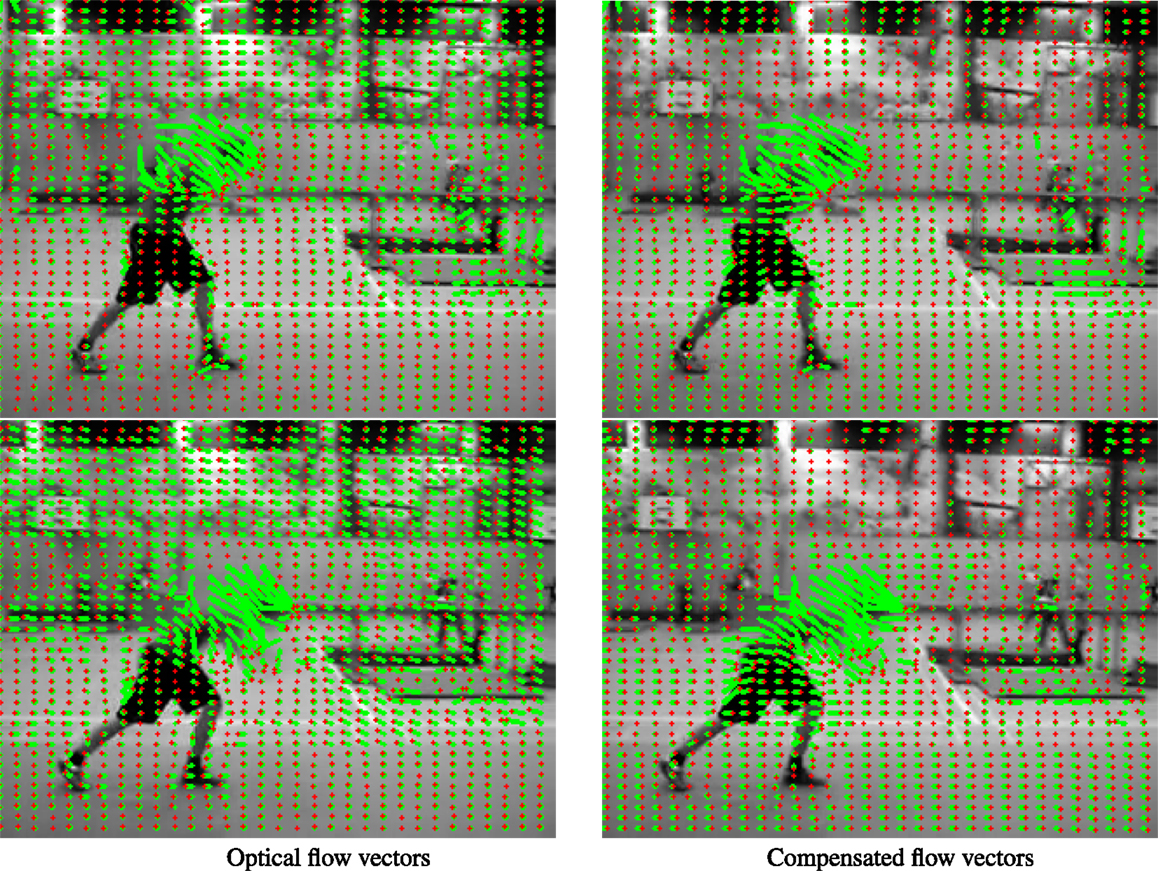
Figure 1. Optical flow field vectors (shown as green vectors with red end points) before and after dominant motion compensation. Most of the flow vectors on the static background due to camera motion are suppressed after compensation. One of the contributions of this work is to show that compensating for the dominant motion is beneficial for most of the existing descriptors used for action recognition. Figure from Jain et al. (2013).

The work presented in this paper is extension of Jain et al. (2013) with the following additions:

• More details of DCS descriptor are given with visual illustrations.

• Higher-order encoding Fisher vector is also used for the video representation.

• We present action classification results when the descriptor from optical flow is combined with the descriptors from the proposed compensated flow.

• Experimental results on a larger UCF101 dataset with 101 action classes.

We organized the paper into 9 sections where Section 3 introduces the motion properties considered in the article; Section 4 covers the classification scheme and datasets for our evaluation; Section 5 revisits popular descriptors through dominant motion compensation; Section 6 displays our novel DCS descriptor; Section 7 is about the performance improvement through VLAD and Fisher encoding techniques; Section 8 provides a comparison with the state-of-the-art; finally, Section 9 concludes the paper.

2. Related Work

In recent years, video action classification has advanced considerably both in terms of performance and on larger and more challenging datasets. Much of the credit goes to better video representation with robust motion descriptors and their higher-order encodings. Examples of motion descriptors that are robust to modest appearance and motion changes are as follows: MBH (Dalal et al., 2006; Wang et al., 2011), HOG (Dalal and Triggs, 2005), HOF (Laptev et al., 2008), Trajectory descriptor (Wang et al., 2011), HOG3D (Kläser et al., 2008), and 3D-SIFT (Scovanner et al., 2007). The descriptors can be computed at feature points sampled as spatio-temporal interest points (Laptev and Lindeberg, 2003), densely (Willems et al., 2008; Shi et al., 2013) or along the trajectories (Matikainen et al., 2009; Wang et al., 2011; Gaidon et al., 2012; Jiang et al., 2012). The effectiveness of descriptors depends on the sampling approach to a large extent: the best results were obtained along the trajectories (Wang et al., 2011; Jain et al., 2013). These descriptors are encoded and aggregated into a single vector global representation of the given video. The most popular choices for encoding are the following: bag of words, Fisher vector (Perronnin et al., 2010) and VLAD (Jégou et al., 2010). Improved performance is obtained by higher-order encodings of Fisher vector (Oneata et al., 2013; Wang and Schmid, 2013), VLAD (Jain et al., 2013), and their adaptations (Peng et al., 2014a,b,c; Wu et al., 2014).

Descriptors are put in to a classifier, such as SVM, after aggregation of local descriptors in global video representations. Video data exhibit visual patterns of motion and motion boundaries also in addition to appearance when compared to static images. Therefore, multiple descriptors are extracted and combined to capture different aspects for action recognition in a typical setting. This pipeline and involved techniques have been extremely successful due to their excellent performance as well as their practical simplicity. Peng et al. (2014c) proposed a two-layer nested Fisher vector encoding called stacked Fisher vectors where the first layer encodes the descriptors from large sub-volumes using Fisher vectors. These sub-volume Fisher vectors are compressed and aggregated again in the second layer. Peng et al. (2014b) proposed a version of VLAD leveraging higher-order statistics, diagonal covariance, and skewness. Their approach learned the codebook in a supervised manner to further improve performance. Ciptadi et al. (2014) introduced a novel way to represent an action as a set of movement pattern histograms that encode the global temporal dynamics of the action, slightly deviating from the above pipeline.

Hoai and Zisserman (2014) proposed a technique that addresses temporal interval ambiguity of actions by learning a classifier score distribution over video subsequences. They also showed that action classification is improved by learning a classifier for the relative values of action scores, capturing the correlation and exclusion between action classes. Kantorov and Laptev (2014) addressed the issue of speed of action classification methods at the cost of minor reduction in the accuracy. They used motion information from video compression and significantly improved the speed of video feature extraction, encoding and action classification. Narayan and Ramakrishnan (2014) exploited the interaction between different object-part motions to extract additional information about the actions. They proposed a causality-based approach for quantifying the interactions to aid action classification.

Another important aspect of recognizing actions is camera motion compensation as first outlined in Piriou et al. (2006). The motion compensation mechanism employed in Kliper-Gross et al. (2012) is tailor-made to the Motion Interchange Pattern encoding technique. The Motion Boundary Histogram (MBH) of Wang et al. (2011) is a more recent approach based on the flow gradient to suppress constant motion. Even though it does not handle the camera motion per se, it proves to be robust to it. Uemura et al. (2008) use an advanced and robust (RANSAC) method to estimate camera motion. They segment the color image into regions first, which correspond to planar parts in the scene, and they estimate dominant homographies to update motion associated with local features. Wu et al. (2011) apply a very different view – they decompose motion at the level of trajectories.

Our work differs from the above efforts as we do not only use compensated motion for extracting trajectories but also for computing motion descriptors for action recognition. The most similar work to our dominant motion compensation approach (Jain et al., 2013) is the recently proposed method of Wang and Schmid (2013), who adopt the idea of handling camera motion for improving motion trajectories and descriptors; however, they propose different means to achieve it. We further discuss and compare our results with their approach in Section 8.

3. Motion Separation and Kinematic Features

In this section, we describe how the dominant and residual motions are separated, which typically covers the segregation of the movement of the camera from independent actions. Our goal is not only to recover the 3D camera motion itself but also to focus on computing the dominant motion between successive frames. We explain how we estimate the dominant motion and employ it to compensate for the camera motion.

3.1. Estimating Dominant Motion

The dominant motion in the image is represented by a 2D parametric motion model. Among polynomial motion models, we consider the 2D affine motion model. Simplest motion models such as the four-parameter model formed by the combination of 2D translation, 2D rotation, and scaling, or more complex ones such as the eight-parameter quadratic model (equivalent to a homography), could be selected as well. The affine model provides a good trade-off between accuracy and efficiency, which is of primary importance when processing a huge video database. It does have limitations since it implies at least a single plane assumption for the static background. This happens without penalizing (especially for outdoor scenes) if differences in depth remain moderated with respect to the distance to the camera. The affine flow vector at point p = (x,y) and at time t, is defined as:

$w_{\text{aff}}\left(p,t\right)=\left[\begin{array}{c}{c}_1\left(t\right)\hfill \\ c_2\left(t\right)\hfill \end{array}\right]+\left[\begin{array}{cc}{a}_1\left(t\right)\hfill & a_2\left(t\right)\hfill \\ a_3\left(t\right)\hfill & a_4\left(t\right)\hfill \end{array}\right]\left[\begin{array}{c}{x}_t\hfill \\ y_t\hfill \end{array}\right].$ (1)

u_aff(p,t) = c₁(t) + a₁(t)x_t + a₂(t)y_t and v_aff(p,t) = c₂(t) + a₃(t)x_t + a₄(t)y_t are horizontal and vertical components of w_aff(p,t), respectively.

We compute the affine flow with the publicly available Motion2D software¹ (Odobez and Bouthemy, 1995) that implements a real-time robust functional minimization. More precisely, the algorithm minimizes with respect to the model parameters the following energy function:

$J\left(\mathrm{\theta }\right)={\displaystyle \sum _{p\hspace{0.17em}\in \mathrm{\hspace{0.17em}\Omega }}}\mathrm{\hspace{0.17em}\rho }\left(I\left(p+w_{\text{aff}}\left(p,t\right)+1\right)-I\left(p\right)\right)$ (2)

where ρ is a robust penalty function (in practice, the Tukey function), I is the image intensity, and Ω denotes the image domain. Minimizing equation (2) requires an iterative algorithm, namely the Iteratively Reweighted Least Squares (IRLS). The minimization is achieved within a multiresolution incremental estimation framework for handling large displacements.

3.2. Compensating Camera Motion

Let us denote the optical flow vector at point p at time t as w(p,t) = (u(p,t), v(p,t)). We introduce the flow vector ω(p,t) obtained by removing the affine flow vector from the optical flow vector:

$\mathrm{\omega }\left(p,t\right)=w\left(p,t\right)-w_{\text{aff}}\left(p,t\right).$ (3)

The dominant motion [estimated as w_aff(p,t)] is usually caused by the camera motion. Equation (3) amounts up to compensating or completely canceling camera motion in such scenarios, however, please note that that this does not always hold true. For example, in case of moving camera with close-up on a moving actor, the dominant motion is the affine estimation of the combination of the apparent actor motion and the camera motion. The interpretation of the motion compensation output is not as straightforward in this case; however, the resulting ω-field still exhibits different patterns for foreground action and the background. Even when the camera is static, the affine model cannot completely account for the actor’s complex motion. As a consequence, there is no major depletion of the action of interest in the residual or compensated motion. We refer to the “compensated” flow as ω-flow in the rest of the article.

The computed optical flow and the ω-flow are shown in Figure 1 where the affine motion model appropriately accounts for the motion induced by the camera movement, i.e., the dominant motion in the image pair.

The compensated flow vectors in the background are close to null and the compensated flow corresponding to the actors in the foreground is inflated. The experiments presented throughout the present article establish that effective separation between dominant and residual motions is a valuable addition to the field of action recognition. As explained in Section 5, we compute local motion descriptors, such as HOF, both on the optical flow and the ω-flow. This enables us to explicitly and directly characterize scene motion.

4. Datasets and Evaluation

In addition to the introduction to the datasets used for the evaluation, the current section is meant to present the bag-of-feature model and the classification scheme used to encode the descriptors.

4.1. Hollywood 2

The Hollywood 2 (Marzalek et al., 2009) dataset contains 1,707 video clips from 69 movies representing 12 action classes. One example is for each class is shown in Figure 2. The dataset is divided into a training set and a test set of 823 and 884 samples, respectively. For each class, average precision (AP) and the mean of APs (mAP) were used for evaluation, according to the standard protocol of this benchmark.

FIGURE 2

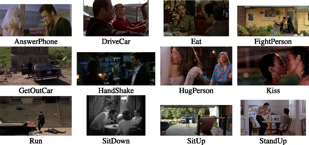
Figure 2. Examples from Hollywood 2 (Marzalek et al., 2009) dataset, 1 for each of the 12 classes.

4.2. HMDB51

The HMDB51 (Kuehne et al., 2011) is a large dataset containing 6,766 video clips extracted from various sources ranging from movies to YouTube. It consists of 51 action classes, each having at least 101 samples. A variety of action categories are covered including the regular day-to-day actions, sports activities, and ones containing a significantly lower amount of motion. Figure 3 displays some examples of these. We follow the evaluation protocol of Kuehne et al. (2011) and use three train/test splits, each with 70 training and 30 testing samples per class. The average classification accuracy is computed over all classes.

FIGURE 3

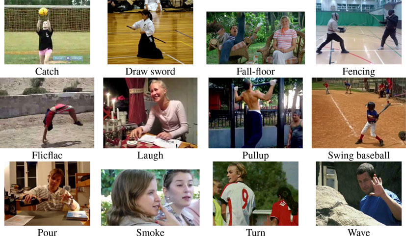
Figure 3. Examples from HMDB51 (Kuehne et al., 2011) dataset for a few of 51 classes.

The HMDB51 dataset was released in two editions, out of which we opted for the original version given that most works in the action recognition field rely on this one, and it also provides a more challenging problem to solve compared to the updated version.

4.3. Olympic Sports

With 783 samples in 16 sports action classes, the Olympic Sports dataset (Niebles et al., 2010) originates from YouTube as well. Figure 4 provides an example of each class. There are 17–56 training samples and 4–11 test samples per class provided. Adhering to the standard choice, we used the mean AP for the evaluation.

FIGURE 4

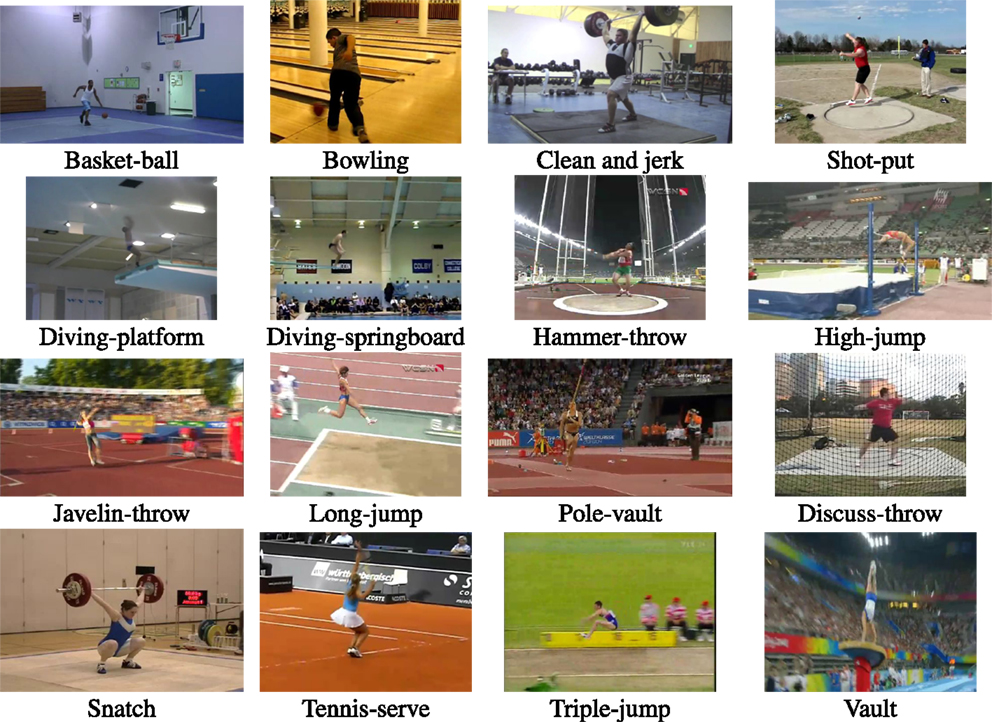
Figure 4. Examples from Olympic Sports (Niebles et al., 2010) dataset, 1 for each of the 16 classes.

4.4. UCF101

The UCF101 dataset (Soomro et al., 2012) is a large action recognition dataset containing 13,320 videos and includes 101 action classes. It has large variations (camera motion, appearance, scale, etc.) and exhibits a lot of diversity in terms of actions. Some of examples are shown in Figure 5. We perform evaluation on the three given train/test splits and report the mean average accuracy over all classes.

FIGURE 5

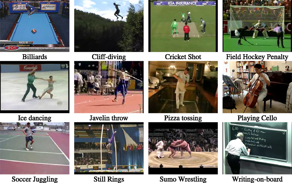
Figure 5. Examples from UCF101 (Soomro et al., 2012) dataset for a few of 101 classes.

4.5. Bag of Features and Classification Setup

We first adopt the standard BOF (Sivic and Zisserman, 2003) approach to aggregate all kinds of descriptors. This produces a vector that serves as the video representation. The codebook is constructed for each type of descriptor separately by the k-means algorithm. Following a common practice in the literature (Wang et al., 2009, 2011; Ullah et al., 2010), the codebook size is set to k = 4,000 elements. Please note that in Section 7, we will consider higher order encoding techniques. For the classification, we use a non-linear SVM with χ²-kernel. When combining different descriptors, we simply add the kernel matrices, as done in Ullah et al. (2010):

$K\left(x_i,x_j\right)=\exp \left(-{\displaystyle \sum _c}\frac{\mathrm{\hspace{0.17em}1}}{{\mathrm{\gamma }}^c}D\left(x_i^c,x_j^c\right)\right),$ (4)

where $D\left(x_i^c,x_j^c\right)$ is χ² distance between video $x_i^c$ and $x_j^c$ with respect to c-th channel, corresponding to c-th descriptor. The quantity γ^c is the mean value of χ² distances between the training samples for the c-th channel. The multi-class classification problem that we tackle with is addressed by applying a one-against-rest approach.

5. Compensated Descriptors

The current section describes how the compensation of the dominant motion is exploited to improve the quality of descriptors encoding the motion and the appearance around spatio-temporal positions, hence the term “compensated descriptors.” We commence by the review of local descriptors (Dollar et al., 2005; Laptev et al., 2008; Marzalek et al., 2009; Wang et al., 2009, 2011) used here along with dense trajectories of Wang et al. (2011). Afterwards, we use motion flow compensation in two different stages of the descriptor computation: in the tracking and the description part.

5.1. Dense Trajectories and Local Descriptors

Employing dense trajectories to compute local descriptors is one of the state-of-the-art approaches for action recognition. Wang et al. (2011) showed that when local descriptors are computed over dense trajectories, its performance improves considerably compared to when computed over spatio-temporal features (Wang et al., 2009).

Dense Trajectories of Wang et al. (2011) are obtained by tracking densely sampled points using optical flow fields. For optical flow computation, an efficient algorithm by Farnebäck (2003) was applied. First of all, feature points are sampled from a dense grid with step size of 5 pixels and over 8 scales. Each feature point p(t) = (x(t), y(t)) at frame t is then tracked to the t + 1^th frame by median filtering in the optical flow field F = (u(t),v(t)) as follows:

$p\left(t+1\right)=\left(x\left(t+1\right),y\left(t+1\right)\right)=\left(x\left(t\right),y\left(t\right)\right)+\left(M\ast F\right){|}_{\left(\overline{x}\left(t\right),ȳ\left(t\right)\right)},$ (5)

where M is the kernel of median filtering and $\left(\overline{x}\left(t\right),ȳ\left(t\right)\right)$ is the rounded position of (x(t),y(t)). The tracking is limited to L frames, with L = 15 in practice, to avoid any drifting effect. Excessively short trajectories and trajectories exhibiting sudden large displacements are removed as they induce artifacts. Trajectories must be understood here as tracks in the space-time volume of the video.

Local descriptors are computed within a space-time volume around each trajectory. There are four types of descriptors that are computed to encode the shape of the trajectory, the local motion pattern and its appearance. These descriptors are: Trajectory (Wang et al., 2011), HOF (Laptev et al., 2008), MBH (Dalal et al., 2006), and HOG (Dalal and Triggs, 2005). All the above descriptors depend on the flow field used for point tracking. The flow-field is further required for the descriptor computation of HOF and MBH:

1. The Trajectory descriptor encodes the shape of the trajectory represented by the normalized relative coordinates of the successive points forming the trajectory. It directly depends on the dense flow used for tracking points.

2. Histogram of optical Flow (HOF) is computed using the orientations and magnitudes of the flow field.

3. Motion boundary histogram (MBH) is designed to capture the gradient of horizontal and vertical components of the flow. The motion boundaries encode the relative pixel motion and therefore suppress constant motion.

4. Histogram of oriented gradients (HOG) encodes the appearance by using the intensity gradient orientations and magnitudes. Formally, HOG is not a motion descriptor, yet the position where the descriptor is computed depends on trajectory shape.

Similarly to Wang et al. (2011), volume around each trajectory is divided into a 2 × 2 × 3 space-time grid. The orientations are quantized into 8 bins for HOG and 9 bins for HOF (with one additional zero bin). The horizontal and vertical components of MBH are separately quantized into 8 bins each.

5.2. Impact of Motion Compensation

The present section analyses and evaluates the impact of our compensated motion on the Hollywood 2 and HMDB51 datasets. The compensated flow is denoted by ω-flow (for details, please see Section 3.1). Both the optical flow and the ω-flow are considered in the tracking and descriptor computation stages leading to a different set of trajectories (referred as ω-trajectories) and descriptors. In Figure 6, a side-by-side demonstration displays the trajectories obtained using the optical flow, those with the affine flow, and the ω-trajectories, respectively. The input video refers to a man walking away from a car; the camera is following the man walking to the right, thus inducing a global apparent motion to the left in the video. When using the optical flow, the computed trajectories display the combination of the two components as shown in Figure 6A, which impedes characterizing the action of interest. Contrasting this, the ω-trajectories plotted in Figure 6C are more active on the actor moving in the foreground, while those computed with affine flow (shown in Figure 6B) now enhance static parts of the scene since they are now mainly parallel to the time axis. The ω-trajectories are therefore more relevant for action recognition, since they are more regularly and more exclusively following the actor’s motion.

FIGURE 6

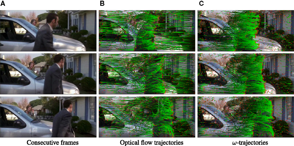
Figure 6. Trajectories obtained from optical and compensated flows. The green tail is the trajectory over the last 15 frames with red dot indicating the current frame. The trajectories are sub-sampled for the sake of clarity. The frames are shown at an interval of 5 frames. Figure from Jain et al. (2013). (A) Consecutive frames, (B) Optical flow trajectories, and (C) ω-trajectories.

Another example sequence of HandShake action is shown in Figure 7. The camera is following the person in black on the left moving toward another person on the right. This induces global motion toward the left as displayed by the trajectories from affine flow in the middle of the figure. As a result, there are several trajectories emanating from optical flow between the two figures shaking hands, i.e., in the background. After motion compensation, most of the trajectories in the background are suppressed and the resulting ω-trajectories are exclusively following the action of interest.

FIGURE 7

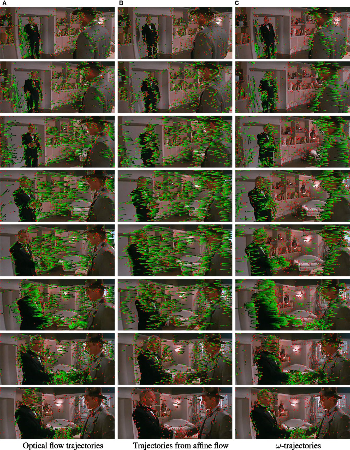
Figure 7. The frame sequence of action HandShake with trajectories obtained from optical, affine, and compensated flows. The green tail is the trajectory taken over fifteen frames with the red dot indicating the current frame. The trajectories are sub-sampled for the sake of clarity. The frames are shown at an interval of five frames. Note that many trajectories in the background are suppressed in ω-trajectories. (A) Optical flow trajectories, (B) trajectories from affine flow, and (C) ω-trajectories.

5.2.1. Impact On Trajectory and HOG Descriptors

Table 1 reports the impact of the ω-trajectories on the Trajectory and the HOG descriptors by comparing with the baseline method of Wang et al. (2011). Both improved versions perform significantly better by 3–4% of mAP on the two datasets. When improved by ω-flow, we name the descriptors as ω-Trajdesc and ω-HOG in the rest of the paper.

TABLE 1

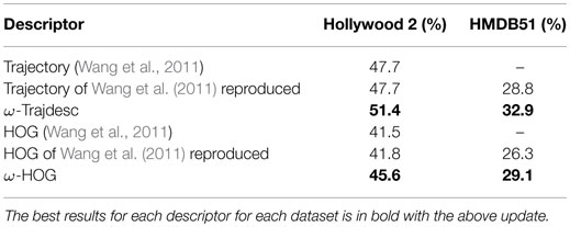
Table 1. Compensation of the optical flow improves trajectory and HOG descriptors.

Even though we expected a better performance of ω-Trajdesc versus the original Trajectory descriptor, the one achieved by ω-HOG seemed to capture more context with the modified trajectories. When the original HOG descriptor is computed from a 2D + t sub-volume, aligned with the corresponding trajectory, it represents the trajectory shape. When using ω-flow, we do not align the video sequence, i.e., we do not warp it according to the affine flow: we instead simply subtract the affine flow from the optical flow. As a result, the ω-HOG descriptor is no longer computed around patches in the space-time volume but around points lying in a patch of the initial feature point, whose size depends on the affine flow magnitude. ω-HOG can be interpreted as a “patch-based” computation that captures more information about the appearance of the background or of the moving foreground.

5.2.2. Impact on HOF

The ω-flow impacts both the trajectory computation used as an input to HOF and the descriptor computation itself. HOF thus can be calculated along both ω-trajectories and those extracted from optical flow. HOF itself can encode ω-flow or optical flow. We furthermore evaluated all variants as well as the combination of both flows during the stage of descriptor computation. Our results are presented in Table 2, which demonstrates the significant improvement obtained through computing the HOF descriptor with the ω-flow instead of the optical flow. The type of applied trajectory – “Tracking optical flow” or “Tracking ω-flow” – has a limited impact in this case. From this point on wards, we only consider the “Tracking ω-flow” case where HOF is computed along ω-trajectories.

TABLE 2

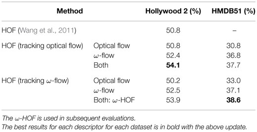
Table 2. Impact of using ω-flow on HOF descriptors: mAP for Hollywood 2 and average accuracy for HMDB51.

Combining the HOF computed from the optical flow and the ω-flow further improves our results. This suggests that the two flow fields are complementary and the affine flow that was subtracted from optical flow brings in additional information. We refer to the combination of HOF computed from the optical flow and the ω-flow using ω-trajectories as the ω-HOF descriptor in the rest of this paper. The ω-HOF descriptor achieves a gain of +3.1% of mAP on Hollywood 2 and of +7.8% on HMDB51 compared to the HOF baseline.

5.2.3. Impact on MBH

Since MBH is computed from gradient of flow and cancels the constant motion, there is no added value in using the ω-flow to compute the MBH descriptors, as shown in Table 3. However, the performance improves by around 1.3% for HMDB51 dataset and drops by around 1.5% for Hollywood 2 by tracking ω-flow. This relative performance depends on the encoding technique. Section 7 elaborates on this further in the context of higher-order encoding schemes discussed in the section.

TABLE 3

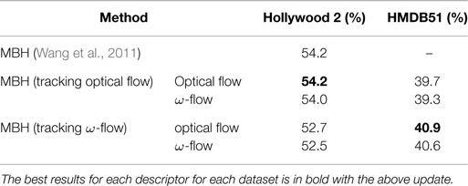
Table 3. Impact of using ω-flow MBH descriptors: mAP for Hollywood 2 and average accuracy for HMDB51.

5.3. Summary of Compensated Descriptors

In Table 4, we summarize the refined versions of the descriptors, which improve considerably with the noticeable exception of ω-MBH with its mixed performance relying on a bag-of-features encoding scheme.

TABLE 4

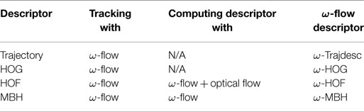
Table 4. Summary of the updated ω-flow descriptors.

Additionally, fewer trajectories are produced through tracking the compensated flow, which creates an advantageous situation. The total number of trajectories decreases by 9.16 and 22.81% on the Hollywood2 and HMDB5, respectively. Please note that exploiting both the optical flow and the ω-flow do not induce an excessive amount of computational overhead, as the latter is obtained from the optical flow and the affine flow, which is computed in real-time and already used to get the ω-trajectories. The only additional computational cost introduced through descriptors in Table 4 is the computation of a second HOF descriptor; however this does not represent a pipeline bottleneck of the extraction procedure due to its relative efficiency.

6. Divergence–Curl–Shear Descriptor

This section introduces a new descriptor encoding the kinematic properties of motion. It is denoted by DCS in the rest of this paper.

6.1. Local Kinematic Features

We mean local first-order differential scalar quantities by kinematic features, which are computed on the flow field. We consider the divergence, the curl (or vorticity) and the hyperbolic terms. They convey useful information on actions in videos through the description on the local physical pattern of the flow and can be computed from the first-order derivatives of the flow at every point p at every frame t as:

$\left\{\begin{array}{cc}\hfill \text{div}\left(p,t\right)\hfill & \hfill =\frac{\mathrm{\partial u}\left(p,t\right)}{\mathrm{\partial x}}+\frac{\mathrm{\partial v}\left(p,t\right)}{\mathrm{\partial y}}\hfill \\ \hfill \text{curl}\left(p,t\right)\hfill & \hfill =\frac{-\mathrm{\partial u}\left(p,t\right)}{\mathrm{\partial y}}+\frac{\mathrm{\partial v}\left(p,t\right)}{\mathrm{\partial x}}\hfill \\ \hfill {\text{hyp}}_1\left(p,t\right)\hfill & \hfill =\frac{\mathrm{\partial u}\left(p,t\right)}{\mathrm{\partial x}}-\frac{\mathrm{\partial v}\left(p,t\right)}{\mathrm{\partial y}}\hfill \\ \hfill {\text{hyp}}_2\left(p,t\right)\hfill & \hfill =\frac{\mathrm{\partial u}\left(p,t\right)}{\mathrm{\partial y}}+\frac{\mathrm{\partial v}\left(p,t\right)}{\mathrm{\partial x}}\hfill \end{array}\right.$ (6)

The divergence is related to axial motion, expansion, and scaling effects, the curl to rotation in the image plane. The hyperbolic terms express the shear of the visual flow corresponding to more complex configuration. We only take shear quantity into account:

$\text{shear}\left(p,t\right)=\sqrt{{\text{hyp}}_1^2\left(p,t\right)+{\text{hyp}}_2^2\left(p,t\right)}.$ (7)

We now propose the DCS descriptor based on the kinematic features: divergence, curl, and shear of the visual motion discussed in this subsection. It is computed on either the optical flow or the compensated flow (i.e., ω-flow).

6.2. DCS Descriptor: Combining Kinematic Features

The spatial derivatives are computed for the horizontal and vertical components of the flow field, which are actually horizontal (MBHx) and vertical (MBHy) parts of MBH descriptor. The input frame and the computed optical flow are shown with these two gradients in Figure 8A. These gradients are in turn used to compute the divergence, curl, and shear scalar values as given by equation (6). Figure 8B shows these three kinematic features computed for the input frame.

FIGURE 8

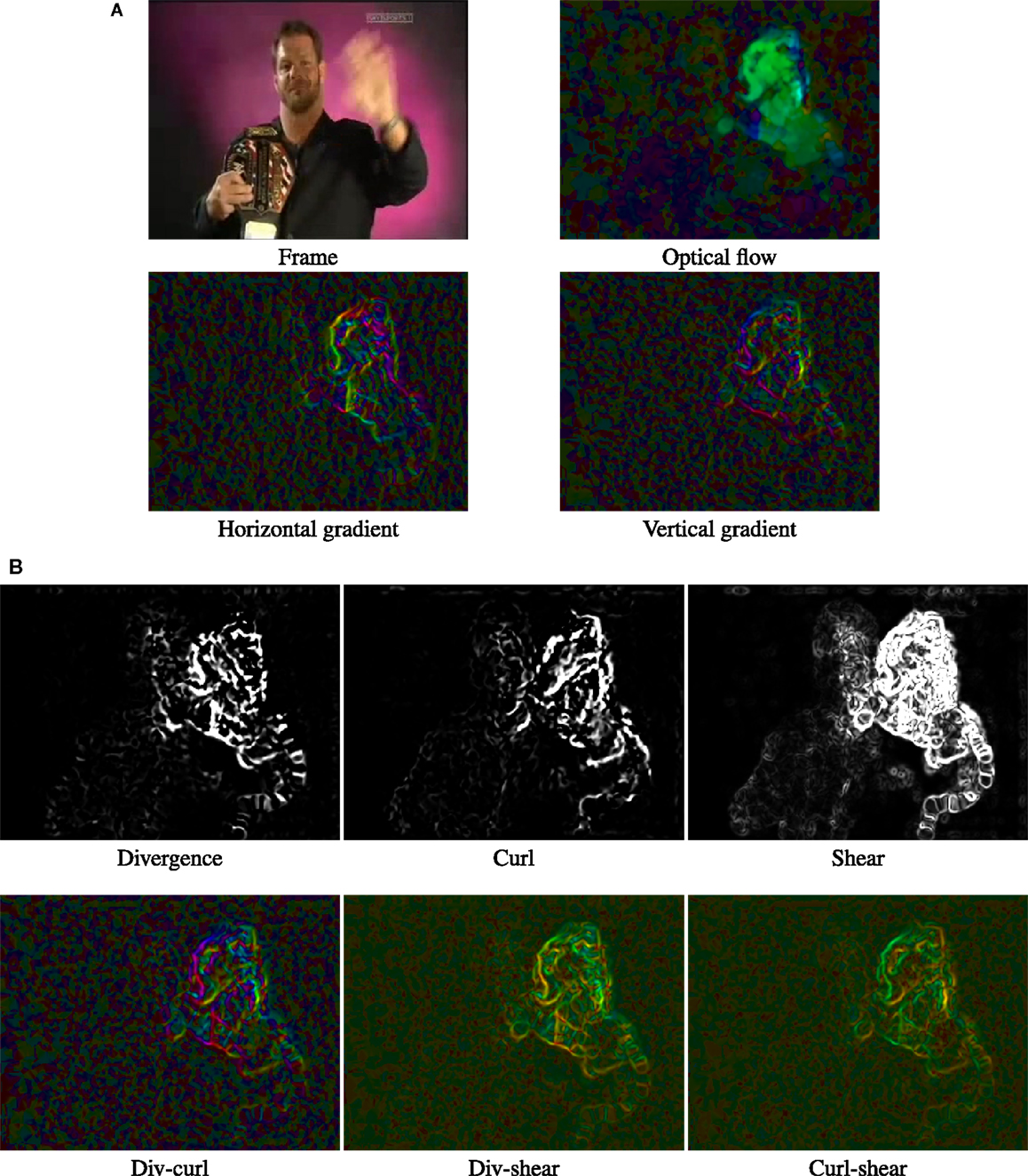
Figure 8. (A) Input frame, optical flow, and the horizontal (MBHx) and vertical (MBHy) gradients of the optical flow. (B) Divergence, curl, and shear computed from the same optical flow above. (C) Joint information captured by each of the 3 possible pairs of kinematic features. Illustration of the information captured by the kinematic features and their 3 possible pair combinations. Scalar quantities, divergence, curl, and shear are shown as gray scale images. For the rest, vector orientation is indicated by color and magnitude by saturation. The example is from HMDB51.

We consider the all 3 possible pairs of kinematic features, namely (div, curl), (div, shear), and (curl, shear). We compute the orientation and magnitude of the 2D vector corresponding to each of these pairs at each pixel. Figure 8C illustrates the information captured by these three pairs. We quantize the orientation into histograms; furthermore, the magnitude was utilized for weighting, similar to SIFT. The motivation behind encoding pairs is that joint distribution of kinematic features conveys extra information compared to when exploiting them independently. Another example is shown in Figure 9 to illustrate the information captured by our DCS descriptor.

FIGURE 9

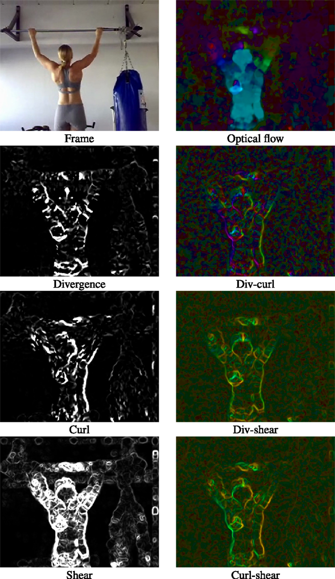
Figure 9. An example of pullup action from HMDB51 to illustrate DCS. Scalar quantities, divergence, curl, and shear are shown as gray scale images. For images in the right column, vector orientation is indicated by color and magnitude by saturation.

6.2.1. Details of Implementation

The computational details, including parameters, are similar to HOG and other popular descriptors, e.g., MBH, HOF. Eight-bin histograms for all three feature pairs or components of DCS were obtained. Given that the shear is always positive: the range of possible angles is 2π for the (div,curl) pair and π for the other ones.

Similarly to the previous section, we computed the DCS descriptor for a space-time volume aligned to a trajectory, as applied to the aforementioned four descriptors. In order to capture the spatio-temporal structure of kinematic features, the volume (32 × 32 pixels and L = 15 frames) is subdivided into a spatio-temporal grid of size n_x × n_y × n_t, with n_x = n_y = 2 and n_t = 3. These parameters are fixed for reasons of consistency. Every histogram represents one cell in the grid for every pair of kinematic features. The resulting dimensionality of local descriptors are equal to n_x × n_y × n_t × 8 × 3 = 288. At the video level, these descriptors are encoded into a single vector representation using either BOF or the higher-order encoding schemes introduced in the next section.

7. Higher-Order Representations: VLAD and Fisher Vector

We herein employ two higher-order encodings for aggregation of local features: VLAD (Jégou et al., 2012) and Fisher vector (Perronnin and Dance, 2007; Perronnin et al., 2010). We introduce them and provide the performance achieved for all the descriptors introduced along the previous sections.

VLAD: It is a descriptor encoding technique that aggregates the descriptors based on a locality criterion in the feature space. Based on available literature search, this technique is considered for action recognition for the first time in our work (Jain et al., 2013). Similar to BOF, VLAD relies on a codebook C = {c₁, c₂, …, c_k} of k centroids learned by k-means. The representation is obtained by summing, for each visual word c_i, the differences x–c_i of the vectors x assigned to c_i, thereby producing a vector representation of length d × k, where d is the dimension of the local descriptors. We use the codebook size, k = 256.

Fisher Vector: The Fisher vector encoding uses Gaussian Mixture Models (GMM) for vocabulary building. It captures the first and second order differences between the image descriptors and the centroids of a GMM. We use the same codebook size as used for VLAD, i.e., 256 Gaussians. We apply Principal Component Analysis (PCA) on the local descriptors and reduce the dimensionality by factor of two, as done in Perronnin et al. (2010). Fisher vector has extra d dimensions per Gaussian to add the second order moments, therefore, the final representation is of 2 × d × k dimensions, where d is the dimension of the local descriptors (after PCA).

Despite this large dimensionality, these representations are efficient because they are effectively compared with a linear kernel. Both of them are post-processed using a component-wise power normalization, which dramatically improves its performance (Jégou et al., 2012). During cross validation of parameter α for power normalization, a value between 0.15 and 0.3 was consistently observed for all the descriptors. Thus, we set this parameter to α = 0.2 in all our experiments. We use one-against-rest linear SVMs for classification everywhere, unless stated otherwise.

7.1. Impact on Existing Descriptors

These higher-order representations encode more information and hence are less sensitive to quantization parameters. This property is interesting in our case, because the quantization parameters involved in the local descriptors have been used unchanged in Section 5 for the sake of direct comparison. When using the ω-flow instead of the optical flow, on which they have initially been optimized (Wang et al., 2011), they might be suboptimal though.

In Table 5, we compare these encodings with BOF. For all the descriptors, VLAD improves over BOF and Fisher further improves over VLAD, with exception of ω-Trajdesc and ω-HOG. BOF performs better than VLAD for these two descriptors on both the datasets, while it just exceeds Fisher for ω-Trajdesc on Hollywood 2. For all other cases, these encodings significantly outdo BOF, especially Fisher with boost of up to 7%.

TABLE 5

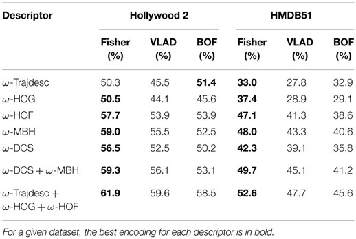
Table 5. Performance of higher-order encodings VLAD and Fisher vector with ω-Trajdesc, ω-HOG, ω-HOF, ω-DCS, and ω-MBH descriptors and their combinations.

Another thing to observe is that the gain is more for the descriptors having larger dimensionality. This is beneficial when combining different descriptors. Consequently, for the two combinations considered: (a) ω-MBH + ω-DCS and (b) ω-Trajdesc + ω-HOG + ω-HOF, VLAD beats BOF, even though BOF did better individually with lower dimensional descriptors. Improvement obtained by Fisher for these combinations is even larger, ranging from 7 to 9% over BOF and around 4 to 5% over VLAD on HMDB51. We also observe that ω-DCS is complementary to ω-MBH and adds to the performance. Yet, DCS is probably not best utilized in the current setting of parameters.

7.2. Combining Trajectories

We have seen that with ω-descriptors results are boosted, this is due to effective separation of dominant motion and residual motion, i.e., camera motion and action-related motion. However, as the camera motion also contains useful information and should not be disregarded. Here, we use this complementary information by combining trajectories from optical flow with ω-trajectories. Table 6 reports the results for Hollywood 2 when:

1. optical flow is used for trajectory extraction and descriptor computation,

2. ω-flow is used for description along ω-trajectories, and

3. the combination of the two. The results are reported for both VLAD and Fisher vector.

TABLE 6

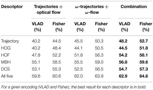
Table 6. Combination of trajectories from optical flow and ω-trajectories with VLAD and Fisher aggregation on Hollywood 2 dataset.

The results are reported for both VLAD and Fisher vector scenarios. Table 7 reports similarly for HMDB51. The performance for each descriptor improves by combining the two types of trajectories, with both encodings and on both datasets. This shows the importance of the camera motion that is integrated with the optical flow.

TABLE 7

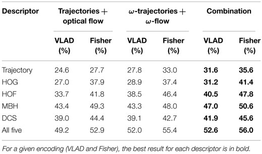
Table 7. Combination of trajectories from optical flow and ω-trajectories with VLAD and Fisher aggregation on HMDB51 dataset.

8. Comparison with the State-of-the-Art

This section reports our results with all descriptors and two types of trajectories combined. We also compare our method with the state-of-the-art.

8.1. Descriptor Combination

In Table 8, we report the results obtained when the descriptors are combined. Since we use Fisher, our baseline is updated, i.e., combination of Trajectory, HOG, HOF and MBH with Fisher vector representation. When DCS is added to the baseline there is an improvement of 0.6 and 1.1% for Hollywood 2 and HMDB51 respectively. The raise in performance by adding DCS is notable considering that there are already four types of descriptors combined. This confirms the contribution of the proposed descriptor. Furthermore, with combination of all five compensated descriptors, we obtain 63.8 and 54.8% on the two datasets.

TABLE 8

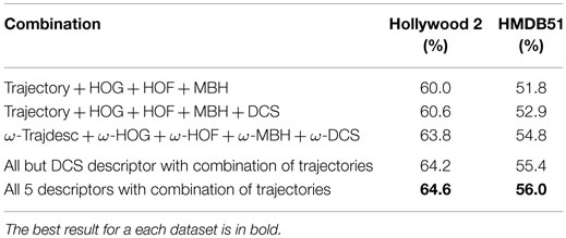
Table 8. Different combinations of descriptors and trajectories using Fisher vector representation.

This is a large improvement even over the updated baseline, which shows that the proposed motion compensation and the way we exploit it are much important for action recognition. When descriptors computed using both types of trajectories are combined as explained in the Subsection 2, there is further increase. Finally, we reach 64.6 and 56.0% for Hollywood 2 and HMDB51, respectively with all five descriptors. These numbers are 64.2 and 55.4% without DCS descriptor, which still adds some value.

We conducted various experiments on these two datasets for in-depth analysis, in particular, the impact of ω-flow, encodings and adding the proposed DCS descriptor. Now, for more elaborative comparison with the state-of-the-art, we also evaluate our approach on UCF101 and Olympic Sports datasets. It is the average accuracy that serves as the evaluation measure for HMDB51 and UCF101, so, we also show the confusion matrices for these two datasets in Figures 10 and 11, respectively. On HMDB51 accuracies are high for most of the classes. A lower performance is caused by understandable confusions for certain classes. These include: “cartwheel” confused with “handstand,” “swing_baseball” confused with “throw,” “smile” confused with “chew,” “sword_exercise” confused with “draw_sword” and the mutual confusion between “sword” and “fencing.” For UCF101, the results are consistently excellent for almost all the classes; one of the rare exceptions being “BasketballDunk” confused as “Basketball,” which is understandable for these instances as well.

FIGURE 10

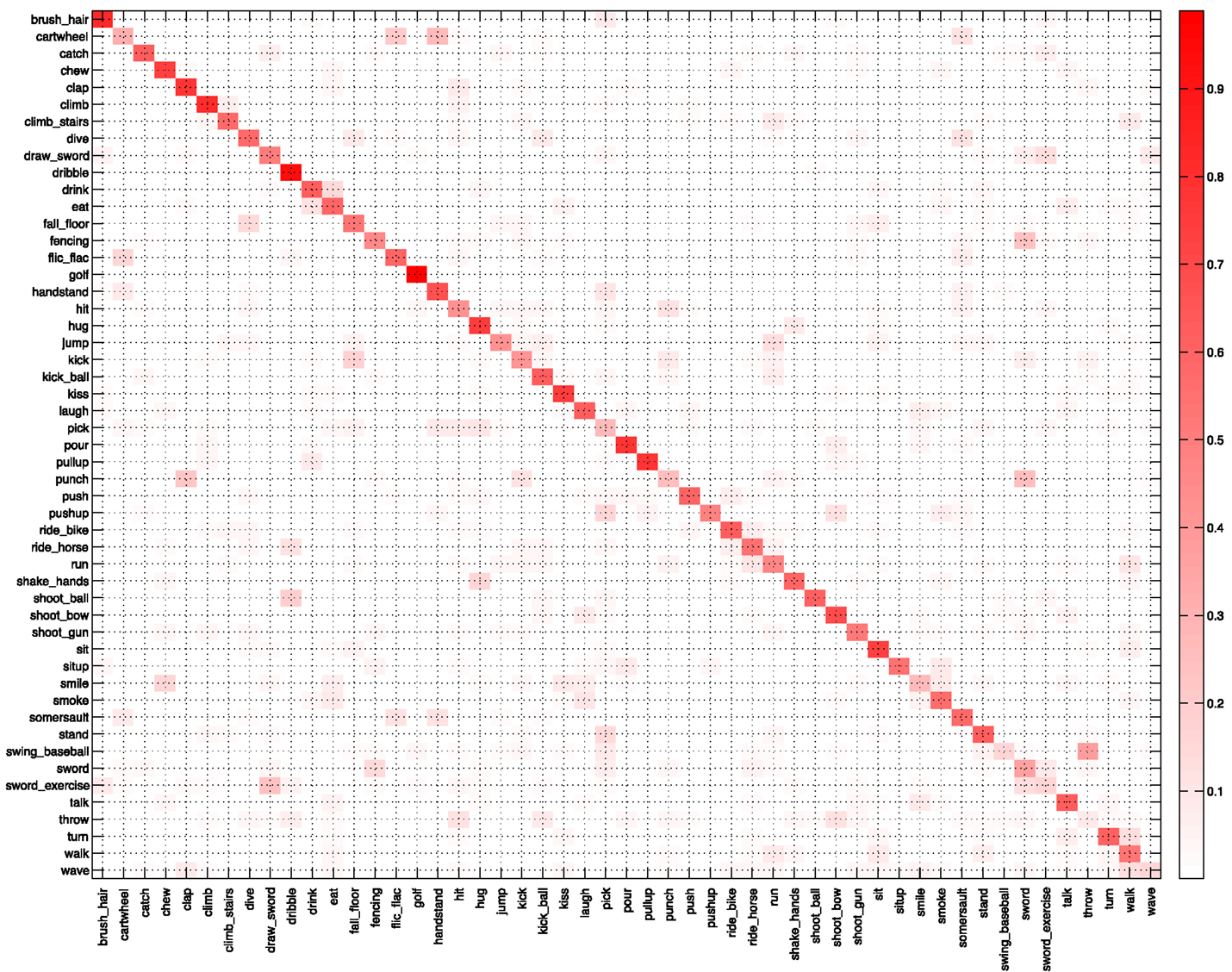
Figure 10. Confusion matrix averaged over the three splits for HMDB51 dataset.

FIGURE 11

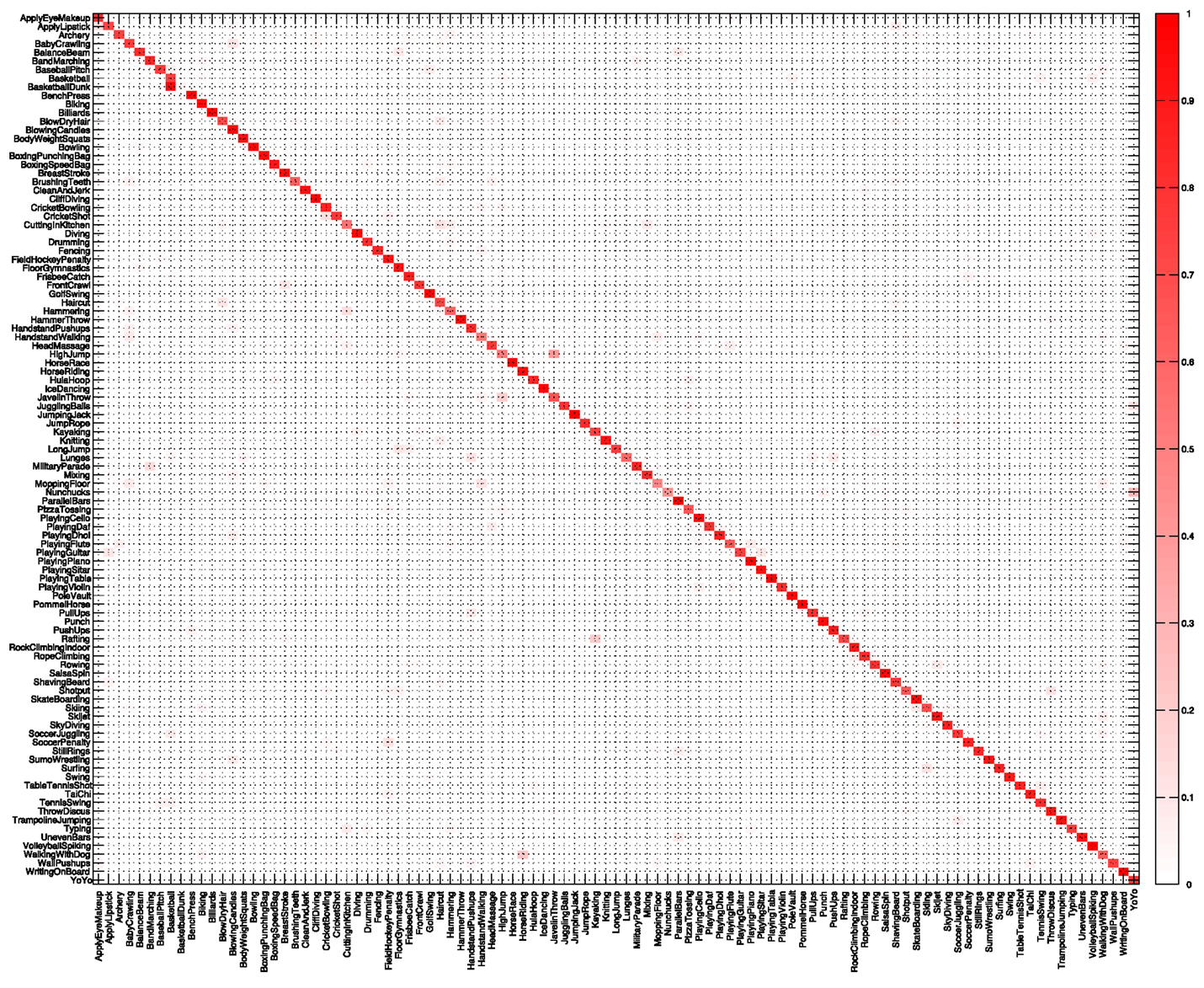
Figure 11. Confusion matrix averaged over the three splits for UCF101 dataset.

The comparison with the state-of-the-art is shown in Table 9. In Jain et al. (2013), our approach outperformed all the previously reported results in the literature. On the HMDB51 dataset in particular, the improvement over the best till-then reported results was more than 11% in average accuracy.

TABLE 9

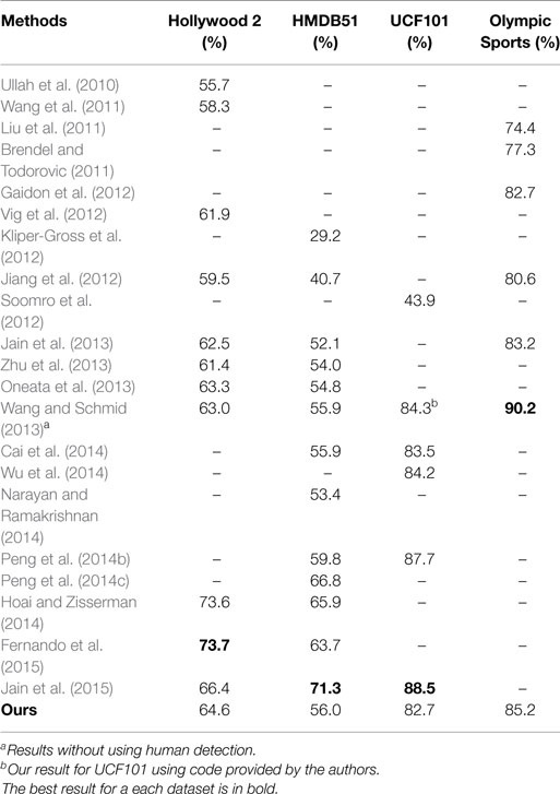
Table 9. Comparison with the state-of-the-art on Hollywood 2, HMDB51, UCF101, and Olympic Sports.

More recently, new methods were proposed (Oneata et al., 2013; Wang and Schmid, 2013; Zhu et al., 2013), which yielded even better results. The approach of Wang and Schmid (2013) is based on the same notion as our ω-trajectories and ω-flow, i.e., to compensate for camera motion. Their camera motion estimation is based on estimating homography using RANSAC between two consecutive frames. To match feature points, they use SURF descriptors in addition to dense optical flow. The inconsistent matches due to human motion are removed by human detection for better camera motion estimation. They use Fisher vector to encode and aggregate local descriptors.

In the current paper, we describe our further improved results relying on a Fisher vector representation and combination of both optical flow trajectories and ω-trajectories. Both these additions to our approach in Jain et al. (2013) have boosted our results to match the results of Wang and Schmid (2013). The performances of the two approaches on Holywood2, HMDB51, and UCF101 are very similar. We obtain a mAP of 85.2% on the Olympic Sports dataset. Our method in some cases performs not as well as improved trajectories of Wang and Schmid (2013). The main reason is that their motion compensation involves warping the second frame according to the camera motion estimation and then recomputing the optical flow for each pair of consecutive frames. This is better suited for MBH descriptor as it is computed from gradient of flow where the constant motion is canceled. As a result, our approach of direct canceling of dominant motion is not as effective, but at the same time it is more efficient as we do not have to compute optical flow again.

The most recent methods of Hoai and Zisserman (2014), Peng et al. (2014b,c), Fernando et al. (2015), and Jain et al. (2015) have achieved larger improvements. In Peng et al. (2014c), Fisher vectors are combined with stacked Fisher vectors (2-layers of Fisher vectors). Temporal ordering in video as motion or as evolution of appearance is exploited in Fernando et al. (2015) and Hoai and Zisserman (2014) for action classification. Object representations are used to assist action recognition in Jain et al. (2015). These approaches use improved trajectories of Wang and Schmid (2013), and we expect these methods to lead to similar results with our ω-trajectories as well.

9. Conclusion

This paper first demonstrates the interest of canceling the dominant motion – predominantly camera motion – for making computed image motion truthful to actions for both the trajectory extraction and descriptor computation. It produces significantly better versions – compensated descriptors – than several state-of-the-art local descriptors for action recognition. The simplicity, efficiency, and effectiveness of our motion compensation approach make it applicable to any action recognition framework based on motion descriptors and trajectories.

The second contribution is the new DCS descriptor derived from the first-order scalar motion quantities specifying the local motion patterns. It captures additional information, which is proven to be complementary to other descriptors. We show that VLAD and Fisher encoding techniques boost action descriptors and overall exhibit a significantly better performance when combining different types of descriptors and trajectories instead of relying on a bag-of-words approach.

Finally, we combined trajectories from optical flow with ω-flow to further improve the results and show that camera motion integrated with the optical flow also contains useful information. Our contributions are all complementary, and when combined lead to the results comparable to the state-of-the-art as demonstrated by our extensive experiments on the Hollywood 2, HMDB51, UCF101, and the Olympic Sports datasets.

Conflict of Interest Statement

The authors declare that the research was conducted in the absence of any commercial or financial relationships that could be construed as a potential conflict of interest. The paper’s short version was published in Jain et al. (2013). The authors declare that they verified the compliance with the copyright requirements of the original publisher.

Footnote

1. ^http://www.irisa.fr/vista/Motion2D/

References

Ali, S., and Shah, M. (2010). Human action recognition in videos using kinematic features and multiple instance learning. IEEE Trans. Pattern Anal. Mach. Intell. 32, 288–303. doi:10.1109/TPAMI.2008.284

PubMed Abstract | CrossRef Full Text | Google Scholar

Aly, R., Arandjelovic, R., Chatfield, K., Douze, M., Fernando, B., Harchaoui, Z., et al. (2013). “The AXES submissions at TrecVid 2013,” in TRECVID Workshop. Gaithersburg, MA.

Google Scholar

Brendel, W., and Todorovic, S. (2011). “Learning spatiotemporal graphs of human activities,” in Proceedings of the IEEE International Conference on Computer Vision. Washington, DC.

Google Scholar

Brox, T., and Malik, J. (2010). “Object segmentation by long term analysis of point trajectories,” in Proceedings of the European Conference on Computer Vision. Crete.

Google Scholar

Cai, Z., Wang, L., Peng, X., and Qiao, Y. (2014). “Multi-view super vector for action recognition,” in Proceedings of the IEEE Conference on Computer Vision and Pattern Recognition. Columbus, OH.

Google Scholar

Ciptadi, A., Goodwin, M. S., and Rehg, J. M. (2014). “Movement pattern histogram for action recognition and retrieval,” in Proceedings of the European Conference on Computer Vision. Zurich.

Google Scholar

Dalal, N., and Triggs, B. (2005). “Histograms of oriented gradients for human detection,” in Proceedings of the IEEE Conference on Computer Vision and Pattern Recognition. Beijing.

Google Scholar

Dalal, N., Triggs, B., and Schmid, C. (2006). “Human detection using oriented histograms of flow and appearance,” in Proceedings of the European Conference on Computer Vision. Graz.

Google Scholar

Dollar, P., Rabaud, V., Cottrell, G., and Belongie, S. (2005). “Behavior recognition via sparse spatio-temporal features,” in VS-PETS. Beijing.

Google Scholar

Farnebäck, G. (2003). “Two-frame motion estimation based on polynomial expansion,” in Scandinavian Conference on Image Analysis. Halmstad.

Google Scholar

Fernando, B., Gavves, E., Oramas, J., Ghodrati, A., and Tuytelaars, T. (2015). “Modeling video evolution for action recognition,” in Proceedings of the IEEE Conference on Computer Vision and Pattern Recognition. Boston, MA.

Google Scholar

Gaidon, A., Harchaoui, Z., and Schmid, C. (2012). “Recognizing activities with cluster-trees of tracklets,” in Proceedings of the British Machine Vision Conference. Surrey.

Google Scholar

Hervieu, A., Bouthemy, P., and Le Cadre, J.-P. (2008). A statistical video content recognition method using invariant features on object trajectories. IEEE Trans. Circuits Syst. Video Technol. 18, 1533–1543. doi:10.1109/TCSVT.2008.2005609

CrossRef Full Text | Google Scholar

Hoai, M., and Zisserman, A. (2014). “Improving human action recognition using score distribution and ranking,” in Asian Conference on Computer Vision. Singapore.

Google Scholar

Jain, M., Jégou, H., and Bouthemy, P. (2013). “Better exploiting motion for better action recognition,” in Proceedings of the IEEE Conference on Computer Vision and Pattern Recognition. Portland, OR.

Google Scholar

Jain, M., van Gemert, J. C., and Snoek, C. G. M. (2015). “What do 15,000 object categories tell us about classifying and localizing actions?,” in Proceedings of the IEEE Conference on Computer Vision and Pattern Recognition.

Google Scholar

Jégou, H., Douze, M., Schmid, C., and Pérez, P. (2010). “Aggregating local descriptors into a compact image representation,” in Proceedings of the IEEE Conference on Computer Vision and Pattern Recognition. San Francisco, CA.

Google Scholar

Jégou, H., Perronnin, F., Douze, M., Sánchez, J., Pérez, P., and Schmid, C. (2012). Aggregating local descriptors into compact codes. IEEE Trans. Pattern Anal. Mach. Intell. 34, 1704–1716. doi:10.1109/TPAMI.2011.235

CrossRef Full Text | Google Scholar

Jiang, Y.-G., Dai, Q., Xue, X., Liu, W., and Ngo, C.-W. (2012). “Trajectory-based modeling of human actions with motion reference points,” in Proceedings of the European Conference on Computer Vision. Florence.

Google Scholar

Kantorov, V., and Laptev, I. (2014). “Efficient feature extraction, encoding and classification for action recognition,” in Proceedings of the IEEE Conference on Computer Vision and Pattern Recognition. Columbus, OH.

Google Scholar

Kläser, A., Marszalek, M., and Schmid, C. (2008). “A spatio-temporal descriptor based on 3d-gradients,” in Proceedings of the British Machine Vision Conference. Leeds.

Google Scholar

Kliper-Gross, O., Gurovich, Y., Hassner, T., and Wolf, L. (2012). “Motion interchange patterns for action recognition in unconstrained videos,” in Proceedings of the European Conference on Computer Vision. Florence.

Google Scholar

Kuehne, H., Jhuang, H., Garrote, E., Poggio, T., and Serre, T. (2011). “Hmdb: a large video database for human motion recognition,” in Proceedings of the IEEE International Conference on Computer Vision. Barcelona.

Google Scholar

Laptev, I., and Lindeberg, T. (2003). “Space-time interest points,” in Proceedings of the IEEE International Conference on Computer Vision. Nice.

Google Scholar

Laptev, I., Marzalek, M., Schmid, C., and Rozenfeld, B. (2008). “Learning realistic human actions from movies,” in Proceedings of the IEEE Conference on Computer Vision and Pattern Recognition. Anchorage, AL.

Google Scholar

Liu, J., Kuipers, B., and Savarese, S. (2011). “Recognizing human actions by attributes,” in Proceedings of the IEEE Conference on Computer Vision and Pattern Recognition. Colorado Springs, CO.

Google Scholar

Lowe, D. (2004). Distinctive image features from scale-invariant keypoints. Int. J. Comput. Vis. 60, 91–110. doi:10.1023/B:VISI.0000029664.99615.94

CrossRef Full Text | Google Scholar

Marzalek, M., Laptev, I., and Schmid, C. (2009). “Actions in context,” in Proceedings of the IEEE Conference on Computer Vision and Pattern Recognition. Miami, FL.

Google Scholar

Matikainen, P., Hebert, M., and Sukthankar, R. (2009). “Trajectons: action recognition through the motion analysis of tracked features,” in Workshop on Video-Oriented Object and Event Classification, ICCV. Kyoto.

Google Scholar

Messing, R., Pal, C. J., and Kautz, H. A. (2009). “Activity recognition using the velocity histories of tracked keypoints,” in Proceedings of the IEEE International Conference on Computer Vision. Kyoto.

Google Scholar

Narayan, S., and Ramakrishnan, K. R. (2014). “A cause and effect analysis of motion trajectories for modeling actions,” in Proceedings of the IEEE Conference on Computer Vision and Pattern Recognition. Columbus, OH.

Google Scholar

Niebles, J. C., Chen, C.-W., and Li, F.-F. (2010). “Modeling temporal structure of decomposable motion segments for activity classification,” in Proceedings of the European Conference on Computer Vision. Crete.

Google Scholar

Odobez, J.-M., and Bouthemy, P. (1995). Robust multiresolution estimation of parametric motion models. J. Vis. Commun. Image Represent. 6, 348–365. doi:10.1006/jvci.1995.1029

CrossRef Full Text | Google Scholar

Oneata, D., Verbeek, J., and Schmid, C. (2013). “Action and event recognition with fisher vectors on a compact feature set,” in Proceedings of the IEEE International Conference on Computer Vision. Sydney.

Google Scholar

Peng, X., Qiao, Y., Peng, Q., and Wang, Q. (2014a). Large margin dimensionality reduction for action similarity labeling. IEEE Signal Process. Lett. 21, 1022–1025. doi:10.1109/LSP.2014.2320530

CrossRef Full Text | Google Scholar

Peng, X., Wang, L., Qiao, Y., and Peng, Q. (2014b). “Boosting vlad with supervised dictionary learning and high-order statistics,” in Proceedings of the European Conference on Computer Vision. Zurich.

Google Scholar

Peng, X., Zou, C., Qiao, Y., and Peng, Q. (2014c). “Action recognition with stacked fisher vectors,” in Proceedings of the European Conference on Computer Vision. Zurich.

Google Scholar

Perronnin, F., and Dance, C. R. (2007). “Fisher kernels on visual vocabularies for image categorization,” in Proceedings of the IEEE Conference on Computer Vision and Pattern Recognition. Minneapolis, MN.

Google Scholar

Perronnin, F., Sánchez, J., and Mensink, T. (2010). “Improving the fisher kernel for large-scale image classification,” in Proceedings of the European Conference on Computer Vision. Crete.

Google Scholar

Piriou, G., Bouthemy, P., and Yao, J.-F. (2006). Recognition of dynamic video contents with global probabilistic models of visual motion. IEEE Trans. Image Process. 15, 3417–3430. doi:10.1109/TIP.2006.881963

PubMed Abstract | CrossRef Full Text | Google Scholar

Schmid, C., and Mohr, R. (1997). Local grayvalue invariants for image retrieval. IEEE Trans. Pattern Anal. Mach. Intell. 19, 530–534. doi:10.1109/34.589215

CrossRef Full Text | Google Scholar

Scovanner, P., Ali, S., and Shah, M. (2007). “A 3-dimensional sift descriptor and its application to action recognition,” in ACM International Conference on Multimedia. Bavaria.

Google Scholar

Shi, F., Petriu, E., and Laganiere, R. (2013). “Sampling strategies for real-time action recognition,” in CVPR. Portland, OR.

Google Scholar

Sivic, J., and Zisserman, A. (2003). “Video Google: a text retrieval approach to object matching in videos,” in Proceedings of the IEEE International Conference on Computer Vision (Nice: IEEE), 1470–1477.

Google Scholar

Snoek, C. G. M., van de Sande, K. E. A., Fontijne, D., Habibian, A., Jain, M., Kordumova, S., et al. (2013). “Mediamill at trecvid 2013: searching concepts, objects, instances and events in video,” in Proceedings of TRECVID. Gaithersburg, MA.

Google Scholar

Soomro, K., Zamir, A. R., and Shah, M. (2012). “UCF101: a dataset of 101 human actions classes from videos in the wild,” in CoRR. Available at: http://arxiv.org/abs/1212.0402

Google Scholar

Sun, C., and Nevatia, R. (2013). “ACTIVE: activity concept transitions in video event classification,” in Proceedings of the IEEE International Conference on Computer Vision. Sydney.

Google Scholar

Sun, J., Wu, X., Yan, S., Cheong, L. F., Chua, T.-S., and Li, J. (2009). “Hierarchical spatio-temporal context modeling for action recognition,” in Proceedings of the IEEE Conference on Computer Vision and Pattern Recognition. Miami, FL.

Google Scholar

Uemura, H., Ishikawa, S., and Mikolajczyk, K. (2008). “Feature tracking and motion compensation for action recognition,” in Proceedings of the British Machine Vision Conference. Leeds.

Google Scholar

Ullah, M. M., Parizi, S. N., and Laptev, I. (2010). “Improving bag-of-features action recognition with non-local cues,” in Proceedings of the British Machine Vision Conference. Aberystwyth.

Google Scholar

Vig, E., Dorr, M., and Cox, D. (2012). “Saliency-based space-variant descriptor sampling for action recognition,” in Proceedings of the European Conference on Computer Vision. Florence.

Google Scholar

Wang, H., Kläser, A., Schmid, C., and Liu, C.-L. (2011). “Action recognition by dense trajectories,” in Proceedings of the IEEE Conference on Computer Vision and Pattern Recognition. Colorado Springs, CO.

Google Scholar

Wang, H., and Schmid, C. (2013). “Action recognition with improved trajectories,” in Proceedings of the IEEE International Conference on Computer Vision. Sydney.

Google Scholar

Wang, H., Ullah, M. M., Kläser, A., Laptev, I., and Schmid, C. (2009). “Evaluation of local spatio-temporal features for action recognition,” in Proceedings of the British Machine Vision Conference. London.

Google Scholar

Willems, G., Tuytelaars, T., and Gool, L. J. V. (2008). “An efficient dense and scale-invariant spatio-temporal interest point detector,” in Proceedings of the European Conference on Computer Vision. Marseille.

Google Scholar

Wu, J., Zhang, Y., and Lin, W. (2014). “Towards good practices for action video encoding,” in Proceedings of the IEEE Conference on Computer Vision and Pattern Recognition. Columbus, OH.

Google Scholar

Wu, S., Oreifej, O., and Shah, M. (2011). “Action recognition in videos acquired by a moving camera using motion decomposition of lagrangian particle trajectories,” in Proceedings of the IEEE International Conference on Computer Vision. Barcelona.

Google Scholar

Zhu, J., Wang, B., Yang, X., Zhang, W., and Tu, Z. (2013). “Action recognition with actons,” in Proceedings of the IEEE International Conference on Computer Vision. Sydney.

Google Scholar