Fortran Code for Generating Random Probability Vectors, Unitaries, and Quantum States

1. Introduction

The generation of random variables has become an essential capability in fields, such as physics, engineering, economics, random search and optimization, artificial intelligence, and game and network theories [see, e.g., Pham and Karaboga (2000), Galam (2002), Garlaschelli and Loffredo (2004), Estrada and Hatano (2008), Perc and Szolnoki (2008), Krioukov et al. (2010), Szolnoki and Perc (2010), Biondo et al. (2013), Javarone and Armano (2013), Rios and Sahinidis (2013), Amaran et al. (2014), Kroese et al. (2014), Javarone (2015), Silver et al. (2016), and references therein]. In Quantum Information Science (QIS), a multidisciplinary field aiming an efficient and far reaching use and manipulation of information, the panorama is not different. The creation of random states and unitaries can be useful for encryption, remote state preparation, data hiding, classical correlation locking, quantum devices and decoherence characterization and tailoring, and for quantumness and correlations quantification (Emerson et al., 2003; Hayden et al., 2004; Galve et al., 2011; Lu et al., 2011; Agarwal and Hashemi Rafsanjani, 2013; Costa and Angelo, 2016; Ma et al., 2015; Maziero, 2015a; Wallman and Emerson, 2015; Bohnet-Waldraff et al., 2016; Rana et al., 2016), to name but a few examples.

Perhaps because of its intuitive syntax and variety of well developed and optimized tools, Fortran, which stands for Formula translation, is the primary choice programing language of many scientists. There are several nice initiatives indicating that it will be continuously and consistently improved in the future (Szymanski, 2007; Metcalf, 2011), what places Fortran as a good option for scientific programing. It is somewhat surprising thus noticing that Fortran does not appear in Quantiki’s list of “quantum simulators.”¹ For more details about codes under active development in other programing languages, see, e.g., Juliá-Díaz et al. (2006), Machnes et al. (2011), Johansson et al. (2012, 2013), Miszczak (2012, 2013), Fritzsche (2014), Gheorghiu (2014) and Johnston (2016). In this article, with the goal of starting the development of a Fortran Library for QIS, we shall explain (free) Fortran codes produced, or organized, for generators of random numbers, probability vectors, unitary matrices, and quantum state vectors and density matrices. Some examples of free software (Free Software Foundation, 1985) programing languages with which it would be interesting to develop similar tools are Python, Maxima, Octave, C, and Java.

This article is structured as follows. We begin (in Section 2) recapitulating some concepts and definitions that we utilize in the remainder of the article. In Section 3, the general description of the code is provided. Reading this section, and the readme file, would be enough for a black box use of the generators. More detailed explanations of each one of them, and of the related options, are given in Sections 4–8. In Section 9, we summarize the article and comment on some tests for the generators.

2. Some Concepts and Definitions

In Quantum Mechanics (QM) (Nielsen and Chuang, 2000; Wilde, 2013), we associate to a system a Hilbert space ℋ. Every state of that system corresponds to a unit vector in ℋ. Observables are described by Hermitian operators O = Σ_j o_j|o_j〉〈o_j|, i.e., o_j ∈ ℝ and |o_j〉 form an orthonormal basis. Born’s rule bridges theory and experiment stating that if the system is prepared in the state |ψ〉 = Σ_j c_j|o_j〉 and O is measured, then the probability for the outcome o_j is p_j = |c_j|² = |〈o_j|ψ〉|². We recall that a set of numbers p_j is regarded as a discrete probability distribution if all the numbers p_j in the set are non-negative (i.e., p_j ≥ 0) and if they sum up to one (i.e., Σ_j p_j = 1). In QM, preparations and tests involving incompatible observables lead to quantum coherence and uncertainty and to the consequent necessity for the use of probabilities.

When we lack information about a system preparation, a complex positive semidefinite matrix (ρ ≥ 0) with unit trace Tr(ρ) = 1, dubbed the density matrix, is the mathematical object used to describe its state (Nielsen and Chuang, 2000; Wilde, 2013). In these cases, if the pure state |ψ_j〉 is prepared with probability p_j, all measurement probabilities can be computed in a succinct way using the density operator ρ = Σ_j p_j|ψ_j〉〈ψ_j|. The ensemble {p_j,|ψ_j〉} leading to a given ρ is not unique. But, as ρ is an Hermitian matrix, we can write its unique eigen-decomposition $\rho ={\sum }_{j=1}^d{r}_j{|r}_j\rangle \langle r_j|$ with r_j being a probability distribution and |r_j〉 an orthonormal basis. We observe that the set of vectors with properties equivalent to those of (r₁, ⋯, r_d), which are dubbed here probability vectors, define the unit simplex.

The mixedness of the state of a system follows also when it is part of a bigger-correlated system. Let us assume that a bi-partite system was prepared in the state |ψ_ab〉. All the probabilities of measurements on the system a can be computed using the (reduced) density matrix obtained taking the partial trace over system b (Maziero, 2016): ρ^a = Tr_b(|ψ_ab〉〈ψ_ab|).

Up to now, we have discussed some of the main concepts of the kinematics of QM. For our purposes here, it will be sufficient to consider the quantum mechanical closed-system dynamics, which is described by a unitary transformation (Nielsen and Chuang, 2000; Wilde, 2013). If the system is prepared in state |ψ〉, its evolved state shall be given by: |ψ_t〉 = U|ψ〉, with UU^† = 𝕀, where 𝕀 is the identity operator in ℋ. The unitary matrix U is obtained from the Schrödinger equation iℏ∂U/∂t = HU, with H being the system Hamiltonian at time t. Between preparation and measurement (reading of the final result), a Quantum Computation (in the circuit model) is nothing but a unitary evolution, which is tailored to implement a certain algorithm.

3. General Description of the Code

The code is divided in five main functionalities that are the random number generator (RNG), the random probability vector generator (RPVG), the random unitary generator (RUG), the random state vector generator (RSVG), and the random density matrix generator (RDMG). Below, we describe in more detail each one of these generators and the related available options.

A module named meths is used in all calling subroutines for these generators in order to share your choices for the method to be used for each task. A short description of the methods and the corresponding options, opt_rxg (with x being n, pv, u, sv, or dm), is included in that module. To call any one of these generators, include call rxg(d,rx) in your program, where d is the dimension of the vector or square matrix rx, which is returned by the generator. If you want, for example, a random density matrix generated using a “standard method” just call rdmg(d,rdm); the same holds for the other objects. If, on the other hand, you want to choose which method is to be used in the generation of any one of these random variables, add use meths after your (sub)program heading, declare opt_rxg as character(10), and add opt_rxg = "your_choice" to your program executable statement section.

4. Random Number Generator

Beforehand we “have” to initialize the RNG with call rng_init(); remember to do that also after changing the RNG. As rn is an one-dimensional double precision array, if you want only one random number (RN), then just set d = 1. As the standard pseudo-random number generator (pRNG), we use the Fortran implementation by Jose Rui Faustino de Sousa of the Mersenne Twister algorithm introduced in Matsumoto and Nishimura (1998). This pRNG has been adopted in several software systems and is highly recommended for scientific computations (Katzgraber, 2010). As less hardware demanding alternatives, we have also included the Gnu’s standard pRNG KISS (Marsaglia and Zaman, 1993) and the Petersen’s Lagged Fibonacci pRNG (Petersen, 1994), which is available on Netlib. The options opt_rng for these three pRNGs are, respectively, "mt", "gnu", and "netlib". The components of rn provided by these pRNG are uniformly distributed in [0, 1]. Because of their use in the other generators, we have also implemented the subroutines rng_unif(d,a,b,rn), rng_gauss(d,rn), rng_exp(d,rn), which return d-dimensional vectors of random numbers with independent components possessing, respectively, uniform in [a,b], Gaussian (standard normal), and exponential probability distributions (see examples in Figure 1).

FIGURE 1

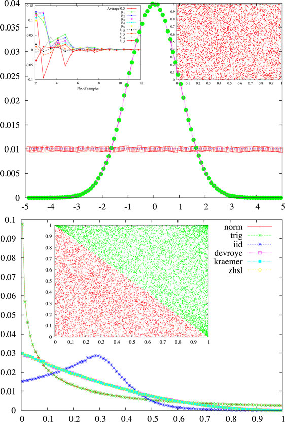
Figure 1. On top: Gaussian and uniform probability densities for one million random numbers generated using the Mersenne Twister random number generator. In the right, inset is shown the 2D scatter plot for 5000 pairs of RNs generated via the Gnu’s RNG. The left inset shows the shifted mean and some moments, μ_j, and correlations, ϵ_j,k, as a function of the number of samples obtained with the Netlib RNG. On bottom: probability density for the first component of one million random probability vectors with dimension d = 4 and generated using the method indicated in the figure (refer to the text for more details). In the inset is shown the 2D scatter plot for the first two components (p₁, p₂) of five thousand RPVs with d = 3 and produced using the ZHSL (red) or the Normalization (green) method [in the last case, the points are (1 − p₁, 1 − p₂)].

5. Random Probability Vector Generator

Once selected the RNG, it can be utilized, for instance, for the sake of sampling uniformly from the unit simplex. That is to say, we want to generate random probability vectors (RPV)

$\overrightarrow{p}=\left(p_1,\cdots ,p_d\right)$ (1)

with p_j ≥ 0 and ${\sum }_{j=1}^d{p}_j=1$; and the picked points $\overrightarrow{p}$ should have uniform density in the unit simplex. In the following, we describe briefly some methods that may be employed to accomplish (approximately) this task.

Let us start with a trigonometric approach to create RPVs (opt_rpvg = "trig"). First, we get the angles θ₀ = 0 and ${\mathrm{\theta }}_j=\text{\hspace{0.17em}arccos}\sqrt{r_j}$ (for j = 1, ⋯, d − 1), with r_j being uniform RNs in [0, 1]. Then, we define the components of the RPV: $p_j={\sin }^2{\mathrm{\theta }}_{j-1}{\mathrm{\Pi }}_{k=j}^{d-1}{\cos }^2{\mathrm{\theta }}_k$ (for j = 1, ⋯, d − 1) and p_d = sin² θ_d−1 (Vedral and Plenio, 1998). To get rid from the bias existing in the generated RPVs, we use a random permutation of {1, 2, ⋯, d} to shuffle its components (Maziero, 2015b).

The normalization method (opt_rpvg = "norm") starts from the defining properties of a probability vector and uses the RNG to draw uniformly p₁ ∈ [0, 1], $p_j\in \left[0,1-{\sum }_{k=1}^{j-1}{p}_k\right]$ (for j = 1, ⋯, d − 1), and set $p_d=1-{\sum }_{k=1}^{d-1}{p}_k$. At last, we use shuffling of the components of $\overrightarrow{p}$ to obtain an unbiased RPV (Maziero, 2015b). A somewhat related method, which is used here as the standard one for the RPVG, was proposed by Zyczkowski, Horodecki, Sanpera, and Lewenstein (ZHSL) in the Appendix A of Zyczkowski et al. (1998), so opt_rpvg = "zhsl." The basic idea is to consider the volume ${\mathrm{\Pi }}_{j=1}^{d-1}\text{d}\left(p_j^{d-j}\right)$ and d − 1 uniform random numbers r_j and to define $p_1=1-r_1^{1∕\left(d-1\right)}$ and $p_j=\left(1-r_j^{1∕\left(d-j\right)}\right)\left(1-{\sum }_{k=1}^{j-1}{p}_k\right)$ (for j = 2, ⋯, d − 1), and finally making $p_d=1-{\sum }_{k=1}^{d-1}{p}_k$.

Other possible approach is taking d independent and identically distributed uniform random numbers r_j (thus opt_rpvg = "iid") and just normalizing the distribution, i.e., $p_j:=r_j∕\left({\sum }_{k=1}^d{r}_k\right)$ (Maziero, 2015b). A related sampling method was put forward in Devroye (1986) (opt_rpvg = "devroye"); see also the Appendix B of Shang et al. (2015). The procedure is similar to the previous one, but with the change that the random numbers r_j are drawn with an exponential probability density. Yet, another way to create a RPV, due to Kraemer (1999) (opt_rpvg = "kraemer") [see also Smith and Tromble (2004) and Grimme (2015)], is to take d − 1 random numbers uniformly distributed in [0, 1], sort them in non-decreasing order, use r₀ = 0 and r_d = 1, and then defining p_j = r_j − r_j–1 for j = 1, ⋯, d. For sorting, we adapted an implementation of the Quicksort algorithm from the Rosetta Code Project.²

With exception of the iid, all these methods lead to fairly good samples. With regard to the similarity of the probability distributions for the components of the RPVs generated, one can separate the methods in two groups: (a) ZHSL, Kraemer, and Devroye and (b) trigonometric and normalization. Concerning the choice of the method, it is worth mentioning that for moderately large dimensions of the RPV, the group (a) excludes the possibility of values of p_j close to one. This effect, which may have unwanted consequences for random quantum states generation, is less pronounced for the methods (b), although here the problem is the appearance of a high concentration of points around the corners p_j = 0 (see Figure 1).

If ℛ (N) is the computational complexity (CC) to generate N RNs and 𝒪 (N) is the CC for N scalar additions, then for d ≫ 1, we have the following estimative: CC(RPVG) ≈ ℛ (d) + 𝒪 (d log d).

6. Random Unitary Generator

A complex matrix U is unitary, i.e.,

$U^{†}U=\mathbb{I},$ (2)

with 𝕀 being the identity matrix, if and only if its column vectors form an orthonormal basis. So, starting with a complex matrix possessing independent random elements that have identical Gaussian (standard normal) probability distributions, we can obtain a random unitary matrix (RU) via the QR factorization (QRF) (Cybenko, 2001; Mezzadri, 2007). We implemented it using the modified Gram–Schmidt orthogonalization (opt_rug = "gso") (Diaconis, 2005; Golub and Van Loan, 2013), which is our standard method for generating random unitaries. We also utilized LAPACK’s implementation of the QRF via Householder reflections (opt_rug = "hhr"), so you will need to have LAPACK installed (Anderson et al., 1999). Random unitaries can be obtained also from a parametrization for U(d). We have implemented a RUG in this way using the Hurwitz parametrization (opt_rug = "hurwitz"); for details, see Zyczkowski and Kus (1994, 1996). Here, a rough estimate for the computational complexity is CC(RUG) ≈ ℛ (d²) + 𝒪 (d⁴).

7. Random State Vector Generator

Pure states of d-dimensional quantum systems are described by unit vectors in ℂ ^d. The computational basis |j〉 = (δ_1j, δ_2j, ⋯, δ _dj) can be used to write any one of these vectors as

$|\mathrm{\psi }\rangle ={\displaystyle \sum _{j=1}^d{c}_j|j\rangle },$ (3)

which are guaranteed to be normalized if ${\sum }_{j=1}^d{\left|c_j\right|}^2=1$. A simple way to create random state vectors (RSVs) is by using normally distributed real numbers to generate the real and imaginary parts of the complex coefficients in equation (3), and afterwards normalizing |ψ〉 (opt_rsvg = "gauss").

Using the polar form for the coefficients in equation (3), $c_j=\left|c_j\right|{\text{e}}^{i{\mathrm{\varphi }}_j}$, and noticing that |c_j|² is a probability distribution, we arrive at our standard method (opt_rsvg = "std") for generating RSVs. We proceed then by defining |c_j|² = : p_j and writing

$|\mathrm{\psi }\rangle ={\displaystyle \sum _{j=1}^d\sqrt{p_j}{e}^{i{\varphi }_j}|j\rangle }.$ (4)

Then, we utilize the RPVG to get $\overrightarrow{p}=\left(p_1,\cdots ,p_d\right)$ and the RNG to obtain the phases (ϕ₁, ⋯, ϕ_d), with ϕ_j uniformly distributed in [0, 2π]. Using these probabilities and phases, we generate a RSV. See examples in Figure 2. For these two first methods, when d ≫ 1, CC(RSVG) ≈ ℛ (d) + 𝒪 (d²).

FIGURE 2

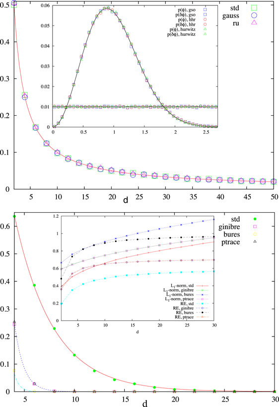
Figure 2. On top: average fidelity, 〈F (|ψ〉, |ϕ〉)〉 = 〈|〈ψ|ϕ〉|²〉, as a function of the dimension d for one thousand pairs of random state vectors generated using the indicated method. The continuous line is for 1/d. In the inset is shown the probability density for the eigen-phases and its spacings (divided by the average) for ten thousand 20 × 20 random unitary matrices. On bottom: probability of finding a positive partial transpose bi-partite state of dimension d = d_ad_b, with d_a = 2, for ten thousand random density matrices produced for each value of d. The continuous lines are the exponential fits, p = αe^{− βd}, with (α, β) being (1.81, 0.26), (18.77, 1.08), and (265.21, 2.08) for, respectively, the std, ginibre (ptrace), and bures method. In the inset is shown the average L₁-norm quantum coherence C_l1(ρ) = Σ_j≠k|ρ_{j, k}| (divided by log₂d) and the relative entropy of quantum coherence C_re(ρ) = S(ρ_diag) − S(ρ), with S(ρ) = −Tr(ρ log₂ρ) being von Neumann’s entropy and ρ_diag is obtained from ρ by erasing its off-diagonal matrix elements, in basis |j〉 (10⁴ samples were produced for each value of d).

In addition to these procedures, we have included yet another RSVG using the first column of a RU (opt_rsvg = "ru"):

$|\mathrm{\psi }\rangle =\left(U_{11},U_{21},\cdots ,U_{d1}\right).$ (5)

8. Random Density Matrix Generator

Our standard method (opt_rdmg = "std") for random density matrix (RDM) generation [see, e.g., Zyczkowski et al. (1998) and Maziero (2015c)], starts from the eigen-decomposition

$\rho ={\displaystyle \sum _{j=1}^d{r}_j|r_j\rangle \langle r_j|}$ (6)

and creates the eigenvalues r_j and the eigenvectors |r_j〉 = U|j〉 using, respectively, the RPVG and RUG described before. So, in this case, CC(RDMG) ≈ CC(RPVG) + CC(RUG) + 𝒪 (d⁶) ≈ ℛ (d²) + 𝒪 (d⁶).

We can also produce RDMs by normalizing matrices with independent complex entries normally distributed, named Wishart or Ginibre matrices (opt_rdmg = "ginibre"),

$\rho =\frac{G{G}^{†}}{\left|\right|G|{|}_2^2},$ (7)

where $\left|\right|G{\left|\right|}_2=\sqrt{\text{Tr}\left(G^{†}G\right)}$ is the Hilbert–Schmidt norm (Zyczkowski and Sommers, 2001; Zyczkowski et al., 2011). A related method, which produces RDMs with Bures measure (opt_rdmg = "bures"), uses

$\rho =\frac{\left(\mathbb{I}+U\right)G{G}^{†}\left(\mathbb{I}+U^{†}\right)}{\left|\right|\left(\mathbb{I}+U\right)G|{|}_2^2},$ (8)

with U being a random unitary (Al Osipov et al., 2010). At last, one can also generate RDMs via partial tracing a random state vector |ψ_ab〉 (Mejía et al., 2015):

$\rho ={\text{Tr}}_b(|{\mathrm{\psi }}_{\mathrm{ab}}\rangle \langle {\mathrm{\psi }}_{\mathrm{ab}}|);$ (9)

so opt_rdmg = "ptrace". See examples in Figure 2.

There are two issues arising from Figure 2 that instantiate the utility of the numerical tool described in this article. The first one regards quantum coherence quantification, which has been rediscovered and formalized in the last few years (Baumgratz et al., 2014; Winter and Yang, 2016). We see that, while the average relative entropy of coherence concentrates around a certain value, the L₁-norm coherence keeps growing with the dimension d. Such kind of qualitative difference, promptly identified in a simple numerical experiment, points toward a path that can be taken in order to identify physically and/or operationally relevant coherence quantifiers. The other issue refers to the too fast concentration of measure reported in Maziero (2015c), and which gains more physical appeal with the too entangled state space reached by the last three RDMGs described in this section.

It seems legitimate regarding the most random ensemble of quantum states as being the one leading to minimal knowledge, which can, by its turn, be identified with maximal symmetry (Hall, 1998). Thus, for pure states, we require such ensemble to be invariant under unitary transformations (UTs), what implies in no preferential direction in the Hilbert space. An ensemble of pure states drawn with probability density invariant under UTs is said to be generated with Haar measure. The same is the case for random unitaries (Mezzadri, 2007). We observe that all random unitary generators and random state vector generators described here produce Haar distributed random objects.

In the general case of density matrices, invariance under UTs only warrants ignorance about direction in the state space, but implies nothing with respect to the eigenvalues distribution. In this regard, in general, different metrics lead to distinct probability densities, which are then used for constructing methods to create random density matrices accordingly. Therefore, as advanced in Hall (1998), this situation calls for the application of physical or conceptual motivations when choosing a RDMG. In this sense, we think that the too fast concentration of measure issue, in conjunction with the well known difficulty of preparing entangled states in the laboratory, favors the standard random density matrix generator described above.

9. Concluding Remarks

To summarize, in this article, we described Fortran codes for the generation of random numbers, probability vectors, unitary matrices, and quantum state vectors and density matrices. Our emphasis here was more on ease of use than on sophistication of the code. This is the starting point for the development of a Fortran Library for Quantum Information Science. In addition to including new capabilities for the generators described here and to optimize the code, we expect to develop this work in several directions in the future. Among the intended extensions are the inclusion of entropy and distinguishability measures, non-classicality and correlation quantifiers, simulation of quantum protocols, and remote access to quantum random number generators. Besides, in order to mitigate the explosive growth in complexity that we face in general when dealing with quantum systems, d = dim ℋ ∝ exp (No. of parties), it would be fruitful to parallelize the code whenever possible.

We performed some simple tests and calculations for verification of the code’s basic functionalities. Some of the results are reported in Figures 1 and 2. The code used for these and other tests is also included and commented, but we shall not explain it here. Several matrix functions are provided in the files matfun.f90 and qnesses.f90. For instructions about how to compile and run the code, see the readme file. In our tests, we used BLAS 3.6.0, LAPACK 3.6.0 (see installation instructions in https://gcc.gnu.org/wiki/GfortranBuild), and the GNU Fortran Compiler version 5.0.0. A MacBook Air Processor 1.3 GHz Intel Core i5, with a 4-GB 1600 MHz DDR3 Memory and Operating System OS X El Capitan Version 10.11.2 was utilized. The code and related files can be downloaded in http://arxiv.org/e-print/1512.05173v1 or https://github.com/jonasmaziero/LibForQ-v1.git [GCC Wiki; Maziero; Maziero (2015)].

Author Contributions

The author performed all the work presented in this article.

Conflict of Interest Statement

The author declares that the research was conducted in the absence of any commercial or financial relationships that could be construed as a potential conflict of interest.

Acknowledgments

This work was supported by the Brazilian funding agencies: Conselho Nacional de Desenvolvimento Científico e Tecnológico (CNPq), under processes 441875/2014-9 and 303496/2014-2, Instituto Nacional de Ciência e Tecnologia de Informação Quântica (INCT-IQ), under process 2008/57856-6, and Coordenação de Desenvolvimento de Pessoal de Nível Superior (CAPES), under process 6531/2014-08. I gratefully acknowledge the hospitality of the Physics Institute and Laser Spectroscopy Group at the Universidad de la República, Uruguay, where this work was completed. I also thank Carlos Alberto Vaz de Moraes Júnior for useful suggestions regarding the creation of Fortran libraries and one of the Reviewers by his/her constructive comments and suggestions.

Supplementary Material

The Supplementary Material for this article can be found online at https://www.frontiersin.org/article/10.3389/fict.2016.00004

Footnotes

1. ^http://www.quantiki.org/wiki/list-qc-simulators
2. ^http://rosettacode.org/wiki/Sorting_algorithms

References

Agarwal, S., and Hashemi Rafsanjani, S. M. (2013). Maximizing genuine multipartite entanglement of N mixed qubits. Int. J. Quantum Inform. 11, 1350043. doi: 10.1142/S0219749913500433

CrossRef Full Text | Google Scholar

Al Osipov, V., Sommers, H.-J., and Zyczkowski, K. (2010). Random Bures mixed states and the distribution of their purity. J. Phys. A Math. Theor. 43, 055302. doi:10.1088/1751-8113/43/5/055302

CrossRef Full Text | Google Scholar

Amaran, S., Sahinidis, N. V., Sharda, B., and Bury, S. J. (2014). Simulation optimization: a review of algorithms and applications. Q. J. Oper. Res. 12, 301. doi:10.1007/s10479-015-2019-x

CrossRef Full Text | Google Scholar

Anderson, E., Bai, Z., Bischof, C., Blackford, S., Demmel, J., Dongarra, J., et al. (1999). LAPACK Users’ Guide, 3rd Edn. Philadelphia: Society for Industrial and Applied Mathematics.

Google Scholar

Baumgratz, T., Cramer, M., and Plenio, M. B. (2014). Quantifying coherence. Phys. Rev. Lett. 113, 140401. doi:10.1103/PhysRevLett.113.140401

PubMed Abstract | CrossRef Full Text | Google Scholar

Biondo, A. E., Pluchino, A., and Rapisarda, A. (2013). The beneficial role of random strategies in social and financial systems. J. Stat. Phys. 151, 607. doi:10.1007/s10955-013-0691-2

CrossRef Full Text | Google Scholar

Bohnet-Waldraff, F., Braun, D., and Giraud, O. (2016). Quantumness of spin-1 states. Phys. Rev. A 93, 012104. doi:10.1103/PhysRevA.93.012104

CrossRef Full Text | Google Scholar

Costa, A. C. S., and Angelo, R. M. (2016). Quantification of Einstein-Podolski-Rosen steering for two-qubit states. Phys. Rev. A 93, 020103(R). doi:10.1103/PhysRevA.93.020103

CrossRef Full Text | Google Scholar

Cybenko, G. (2001). Reducing quantum computations to elementary unitary operations. Comput. Sci. Eng. 3, 27. doi:10.1109/5992.908999

CrossRef Full Text | Google Scholar

Devroye, L. (1986). Non-Uniform Random Variate Generation. New York: Springer.

Google Scholar

Diaconis, P. (2005). What is a random matrix? Not. AMS 52, 1348.

Google Scholar

Emerson, J., Weinstein, Y. S., Saraceno, M., Lloyd, S., and Cory, D. G. (2003). Pseudo-random unitary operators for quantum information processing. Science 302, 2098. doi:10.1126/science.1090790

PubMed Abstract | CrossRef Full Text | Google Scholar

Estrada, E., and Hatano, N. (2008). Communicability in complex networks. Phys. Rev. E Stat. Nonlin. Soft Matter Phys. 77, 036111. doi:10.1103/PhysRevE.77.036111

PubMed Abstract | CrossRef Full Text | Google Scholar

Free Software Foundation. (1985). Available at: https://fsf.org

Google Scholar

Fritzsche, S. (2014). The Feynman tools for quantum information processing: design and implementation. Comput. Phys. Commun. 185, 1697. doi:10.1016/j.cpc.2014.02.003

CrossRef Full Text | Google Scholar

Galam, S. (2002). Minority opinion spreading in random geometry. Eur. Phys. J. B 25, 403. doi:10.1140/epjb/e20020045

CrossRef Full Text | Google Scholar

Galve, F., Giorgi, G., and Zambrini, R. (2011). Orthogonal measurements are almost sufficient for quantum discord of two qubits. EPL 96, 40005. doi:10.1209/0295-5075/96/40005

CrossRef Full Text | Google Scholar

Garlaschelli, D., and Loffredo, M. I. (2004). Fitness-dependent topological properties of the World Trade Web. Phys. Rev. Lett. 93, 188701. doi:10.1103/Phys-RevLett.93.188701

PubMed Abstract | CrossRef Full Text | Google Scholar

GCC Wiki. Building Common Software Packages with Gfortran. Available at: https://gcc.gnu.org/wiki/GfortranBuild

Google Scholar

Gheorghiu, V. (2014). Quantum++–A C++11 quantum computing library. arXiv:1412.4704.

Google Scholar

Golub, G. H., and Van Loan, C. F. (2013). Matrix Computations, 4th Edn. Baltimore: The Johns Hopkins University Press.

Google Scholar

Grimme, C. (2015). Picking a Uniformly Random Point from an Arbitrary Simplex. Technical Report. University of Münster.

Google Scholar

Hall, M. J. W. (1998). Random quantum correlations and density operator distributions. Phys. Lett. A 242, 123. doi:10.1016/S0375-9601(98)00190-X

CrossRef Full Text | Google Scholar

Hayden, P., Leung, D., Shor, P. W., and Winter, A. (2004). Randomizing quantum states: constructions and applications. Commun. Math. Phys. 250, 371. doi:10.1007/s00220-004-1087-6

CrossRef Full Text | Google Scholar

Javarone, M. A. (2015). Is poker a skill game? New insights from statistical physics. EPL 110, 58003. doi:10.1209/0295-5075/110/58003

CrossRef Full Text | Google Scholar

Javarone, M. A., and Armano, G. (2013). Quantum-classical transitions in complex networks. J. Stat. Mech. Theor. Exp. 2013, 04019. doi:10.1088/1742-5468/2013/04/P04019

CrossRef Full Text | Google Scholar

Johansson, J. R., Nation, P. D., and Nori, F. (2012). QuTiP: an open-source python framework for the dynamics of open quantum systems. Comput. Phys. Commun. 183, 1760. doi:10.1016/j.cpc.2012.02.021

CrossRef Full Text | Google Scholar

Johansson, J. R., Nation, P. D., and Nori, F. (2013). QuTiP 2: a python framework for the dynamics of open quantum systems. Comput. Phys. Commun. 184, 1234. doi:10.1016/j.cpc.2012.11.019

CrossRef Full Text | Google Scholar

Johnston, N. (2016). QETLAB: A MATLAB Toolbox for Quantum Entanglement, Version 0.9. Available at: http://www.qetlab.com

Google Scholar

Juliá-Díaz, B., Burdis, J. M., and Tabakin, F. (2006). QDENSIT–a mathematica quantum computer simulation. Comput. Phys. Commun. 174, 914. doi:10.1016/j.cpc.2005.12.021

CrossRef Full Text | Google Scholar

Katzgraber, H. G. (2010). Random numbers in scientific computing: an introduction. arXiv:1005.4117.

Google Scholar

Kraemer, H. (1999). Post on MathForum on December 20. Topic: Sampling Uniformly from the N-Simplex.

Google Scholar

Krioukov, D., Papadopoulos, F., Kitsak, M., Vahdat, A., and Boguna, M. (2010). Hyperbolic geometry of complex networks. Phys. Rev. E Stat. Nonlin. Soft Matter Phys. 82, 036106. doi:10.1103/Phys-RevE.82.036106

PubMed Abstract | CrossRef Full Text | Google Scholar

Kroese, D. P., Brereton, T., Taimre, T., and Botev, Z. I. (2014). Why the Monte Carlo method is so important today. Comput. Stat. 6, 386. doi:10.1002/wics.1314

CrossRef Full Text | Google Scholar

Lu, X.-M., Ma, J., Xi, Z., and Wang, X. (2011). Optimal measurements to access classical correlations of two-qubit states. Phys. Rev. A 83, 012327. doi:10.1103/Phys-RevA.83.012327

CrossRef Full Text | Google Scholar

Ma, Z., Chen, Z., Fanchini, F. F., and Fei, S.-M. (2015). Quantum discord for d ⊗ 2 systems. Sci. Rep. 5, 10262. doi:10.1038/srep10262

CrossRef Full Text | Google Scholar

Machnes, S., Sander, U., Glaser, S. J., de Fouquieres, P., Gruslys, A., Schirmer, S., et al. (2011). Comparing, optimising and benchmarking quantum control algorithms in a unifying programming framework. Phys. Rev. A 84, 022305. doi:10.1103/Phys-RevA.84.022305

CrossRef Full Text | Google Scholar

Marsaglia, G., and Zaman, A. (1993). The KISS Generator. Technical Report. Department of Statistics, Florida State University.

Google Scholar

Matsumoto, M., and Nishimura, T. (1998). Mersenne Twister: a 623-dimensionally equidistributed uniform pseudorandom number generator. ACM Trans. Model. Comput. Sim. 8, 3. doi:10.1145/272991.272995

CrossRef Full Text | Google Scholar

Maziero, J. Fortran Code for Generating Random Probability Vectors, Unitaries, and Quantum States. Available at: https://github.com/jonasmaziero/LibForQ-v1.git

Google Scholar

Maziero, J. (2015). Fortran Code for Generating Random Probability Vectors, Unitaries, and Quantum States. arXiv:1512.05173v1 [quant-ph]. Available at: http://arxiv.org/e-print/1512.05173v1

Google Scholar

Maziero, J. (2015a). Non-monotonicity of trace distance under tensor products. Braz. J. Phys. 45, 560. doi:10.1007/s13538-015-0350-y

CrossRef Full Text | Google Scholar

Maziero, J. (2015b). Generating pseudo-random discrete probability distributions. Braz. J. Phys. 45, 377. doi:10.1007/s13538-015-0337-8

CrossRef Full Text | Google Scholar

Maziero, J. (2015c). Random sampling of quantum states: a survey of methods. Braz. J. Phys. 45, 575. doi:10.1007/s13538-015-0367-2

CrossRef Full Text | Google Scholar

Maziero, J. (2016). Computing partial traces and reduced density matrices. arXiv:1601.07458.

Google Scholar

Mejía, J., Zapata, C., and Botero, A. (2015). The difference between two random mixed quantum states: exact and asymptotic spectral analysis. arXiv:1511.07278.

Google Scholar

Metcalf, M. (2011). The seven ages of Fortran. J. Comput. Sci. Technol. 11, 1.

Google Scholar

Mezzadri, F. (2007). How to generate random matrices from the classical compact groups. Not. AMS 54, 592.

Google Scholar

Miszczak, J. A. (2012). Generating and using truly random quantum states in Mathematica. Comput. Phys. Commun. 183, 118. doi:10.1016/j.cpc.2011.08.002

CrossRef Full Text | Google Scholar

Miszczak, J. A. (2013). Employing online quantum random number generators for generating truly random quantum states in Mathematica. Comput. Phys. Commun. 184, 257. doi:10.1016/j.cpc.2012.08.012

CrossRef Full Text | Google Scholar

Nielsen, M. A., and Chuang, I. L. (2000). Quantum Computation and Quantum Information. Cambridge: Cambridge University Press.

Google Scholar

Perc, M., and Szolnoki, A. (2008). Social diversity and promotion of cooperation in the spatial prisoner’s dilemma game. Phys. Rev. E Stat. Nonlin. Soft Matter Phys. 77, 011904. doi:10.1103/PhysRevE.77.011904

CrossRef Full Text | Google Scholar

Petersen, W. P. (1994). Lagged Fibonacci series random number generators for the NEC SX-3. Int. J. High Speed Comput. 6, 387. doi:10.1142/S0129053394000202

CrossRef Full Text | Google Scholar

Pham, D. T., and Karaboga, D. (2000). Intelligent Optimisation Techniques: Genetic Algorithms, Tabu Search, Simulated Annealing and Neural Networks. London: Springer.

Google Scholar

Rana, S., Parashar, P., and Lewenstein, M. (2016). Trace-distance measure of coherence. Phys. Rev. A 93, 012110. doi:10.1103/PhysRevA.93.012110

CrossRef Full Text | Google Scholar

Rios, L. M., and Sahinidis, N. V. (2013). Derivative-free optimization: a review of algorithms and comparison of software implementations. J. Glob. Optim. 56, 1247. doi:10.1007/s10898-012-9951-y

CrossRef Full Text | Google Scholar

Shang, J., Seah, Y.-L., Ng, H. K., Nott, D. J., and Englert, B.-G. (2015). Monte Carlo sampling from the quantum state space. I. New J. Phys. 17, 043017. doi:10.1088/1367-2630/17/4/043017

CrossRef Full Text | Google Scholar

Silver, D., Huang, A., Maddison, C. J., Guez, A., Sifre, L., van den Driessche, G., et al. (2016). Mastering the game of go with deep neural networks and tree search. Nature 529, 484. doi:10.1038/nature16961

PubMed Abstract | CrossRef Full Text | Google Scholar

Smith, N. A., and Tromble, R. W. (2004). Sampling Uniformly from the Unit Simplex. Technical Report. Johns Hopkins University.

Google Scholar

Szolnoki, A., and Perc, M. (2010). Reward and cooperation in the spatial public goods game. EPL 92, 38003. doi:10.1209/0295-5075/92/38003

CrossRef Full Text | Google Scholar

Szymanski, B. K. (2007). Fortran programming language and scientific programming: 50 years of mutual growth. Sci. Program. 15, 1. doi:10.1155/2007/979872

CrossRef Full Text | Google Scholar

Vedral, V., and Plenio, M. B. (1998). Entanglement measures and purification procedures. Phys. Rev. A 57, 1619. doi:10.1103/PhysRevA.57.1619

CrossRef Full Text | Google Scholar

Wallman, J. J., and Emerson, J. (2015). Noise tailoring for scalable quantum computation via randomized compiling. arXiv:1512.01098.

Google Scholar

Wilde, M. M. (2013). Quantum Information Theory. Cambridge: Cambridge University Press.

Google Scholar

Winter, A., and Yang, D. (2016). Operational resource theory of coherence. arXiv:1506.07975.

Google Scholar

Zyczkowski, K., Horodecki, P., Sanpera, A., and Lewenstein, M. (1998). Volume of the set of separable states. Phys. Rev. A 58, 883. doi:10.1103/PhysRevA.58.883

CrossRef Full Text | Google Scholar

Zyczkowski, K., and Kus, M. (1994). Random unitary matrices. J. Phys. A Math. Gen. 27, 4235. doi:10.1088/0305-4470/27/12/028

CrossRef Full Text | Google Scholar

Zyczkowski, K., and Kus, M. (1996). Interpolating ensembles of random unitary matrices. Phys. Rev. E 53, 319. doi:10.1103/PhysRevE.53.319

CrossRef Full Text | Google Scholar

Zyczkowski, K., Penson, K. A., Nechita, I., and Collins, B. (2011). Generating random density matrices. J. Math. Phys. 52, 062201. doi:10.1063/1.3595693

CrossRef Full Text | Google Scholar

Zyczkowski, K., and Sommers, H.-J. (2001). Induced measures in the space of mixed quantum states. J. Phys. A Math. Gen. 34, 7111. doi:10.1088/0305-4470/34/35/335

CrossRef Full Text | Google Scholar