Monocular, Boundary-Preserving Joint Recovery of Scene Flow and Depth

1. Introduction

Scene flow is the three-dimensional (3D) motion field of the visible environmental surfaces projected on the image domain: at each image point, scene flow is the 3D velocity of the corresponding environmental surface point. It is the time derivative of 3D position. As such, it is a function of both depth and optical flow (Longuet-Higgins and Prazdny, 1981). Scene flow computation has been the focus of several recent studies (Vedula et al., 2005; Huguet and Devernay, 2007; Pons et al., 2007; Wedel et al., 2008; Mitiche and Aggarwal, 2013; Vogel et al., 2013). It is a typical inverse problem best stated by variational formulations (Mitiche and Aggarwal, 2013). Basic variational statements use L² (Tikhonov) regularization. This regularization, which imposes smoothness on the solution, yields linear terms in the Euler–Lagrange equations. This is the case with the scheme described in Mitiche et al. (2015) and of which we describe a generalization in this paper. The scheme improved significantly on others because it needed a single image sequence rather than a stereo stream like other methods. Also, it formulated the problem using an integral functional of two terms: a data fidelity term to constrain the computed scene flow to conform to the image sequence spatiotemporal derivatives and L² regularization terms to constrain the computed scene flow and depth to be smooth, which led to linear Euler–Lagrange equations for the minimization of the objective functional, much like in the Horn and Schunck optical flow formulation (Horn and Schunk, 1981), except that it involved depth and scene flow rather than optical flow. However, L² regularization blurs the computed scene flow and depth boundaries because it imposes their smoothness everywhere. In general, some form of boundary-preserving regularization is necessary. This is particularly true when environmental objects move independently relative to the viewing system. The variation of motion and structure in such a case can be sharp and significant at these objects occluding boundaries, and therefore, accuracy would require that they be preserved by the regularization operator.

Boundary-preserving recovery of scene flow and depth can be specified in various ways (Mitiche and Aggarwal, 2013). For example, instead of the L² norm, one can use the Aubert et al. function (Aubert et al., 1999; Aubert and Kornprobst, 2002) or the L¹ norm. We can also inhibit smoothing across boundaries by joint 3D motion estimation and segmentation (Mitiche and Sekkati, 2006). In this follow-up study of our previous investigation (Mitiche et al., 2015), we apply the L¹ regularization. There are three basic reasons for this choice: (1) the ability of the L¹ constraint to preserve sharp boundaries while penalizing oscillations. This is well suited for “blocky images” which tend to be smooth inside regions, which have sharp significant boundaries, as is, in general, typical of motion fields; (2) in practice, it can be implemented by computationally efficient approximations without affecting the accuracy of results in a noticeable way; and (3) there is a significant body of literature in its support, particularly in image restoration (Vogel, 2002).

Recovery of scene flow and depth uses the image sequence spatiotemporal derivatives. The study in Mitiche et al. (2015) computed derivatives by a variational formulation, which used an anti-differentiation data fidelity term, and L² regularization. The anti-differentiation term expressed the fact that an image derivative is a function which when integrated gives the image. The present study uses the same anti-differentiation data fidelity term but substitutes L¹ regularization for L² in order, first, to be consistent with the use of L¹ regularization of scene flow and depth and, second, to have the evaluation of the derivatives account for their discontinuities.

We conducted several experiments with real and synthetic data to verify the validity and efficiency of the scheme. We show comparative results that put in evidence the improvements one can obtain by using L¹ rather than L² regularization of depth and motion, as well as by evaluating the image derivatives with L¹ rather than L² regularization.

The remainder of this paper is organized as follows: Section 2 develops the objective functional, and Section 3 describes its minimization. Section 4 shows how the image derivatives are computed. The validation experiments, using synthetic and real image sequences, are described in Section 5. Section 6 contains a conclusion.

2. Formulation

Let I: (x,y,t) → I(x,y,t) be an image sequence, where (x,y) are the spatial coordinates on the bounded image domain Ω, and t ∈ R⁺ designates time. Let (X,Y,Z) be the coordinates of a point P in space and (x,y) the coordinates of its projection. The coordinate system and the imaging geometry are shown in Figure 1. Let U, V, and W be the scene flow coordinate functions. The scene flow and depth linear gradient constraint (Mitiche et al., 2015), which relates the scene flow coordinates U, V, and W and depth Z to the spatiotemporal image is

${\mathit{fI}}_{x}U+{\mathit{fI}}_{y}V-\left({\mathit{xI}}_x+{\mathit{yI}}_y\right)W+I_{t}Z=0,$ (1)

where I_x, I_y, and I_t are the image spatiotemporal derivatives, Z designates depth (Figure 1), and $\left(U,V,W\right)=\left(\frac{\mathit{dX}}{\mathit{dt}},\frac{\mathit{dY}}{\mathit{dt}},\frac{\mathit{dZ}}{\mathit{dt}}\right)$ is the scene flow vector at P. This is a homogeneous linear equation in the variables of scene flow and depth. The homogeneity results from the aperture problem. Multiplication of motion and depth (and structure thereof) by a constant (scale) maintains the equation integrity. One can remove this uncertainty of scale by choosing the depth to be relative to the frontoparallel plane Z = Z₀, for some positive depth Z₀ (Mitiche et al., 2015). Therefore, equation (1) becomes:

${\mathit{fI}}_{x}U+{\mathit{fI}}_{y}V-\left({\mathit{xI}}_x+{\mathit{yI}}_y\right)W+I_t\left(Z-Z_0\right)+I_t{Z}_0=0$ (2)

FIGURE 1

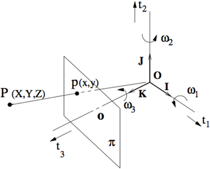
Figure 1. The viewing system is represented by a Cartesian coordinate system (O; X,Y,Z) and central projection through the origin. The Z-axis is the depth axis. The image plane π is orthogonal to the Z-axis at distance f, the focal length, from O.

For notational convenience and economy, we will reuse the symbol Z for depth relative to the frontoparallel pane Z = Z₀, in which case we can write equation (2) as

${\mathit{fI}}_{x}U+{\mathit{fI}}_{y}V-\left({\mathit{xI}}_x+{\mathit{yI}}_y\right)W+I_{t}Z+I_t{Z}_0=0$ (3)

In the formulation of Mitiche et al. (2015), scene flow and relative depth resulted from the minimization of the following L² smoothness regularization functional:

$\begin{array}{l}\mathbf{E}\left(U,V,W,Z|I\right)=\frac{1}{2}{\int }_{\mathrm{\Omega }}({\mathit{fI}}_{x}U+{\mathit{fI}}_{y}V-\left({\mathit{xI}}_x+{\mathit{yI}}_y\right)W+I_{t}Z+I_t{Z}_0{)}^2\mathit{dxdy}\hfill \\ +\frac{\alpha }{2}{\int }_{\mathrm{\Omega }}\left(\mathrm{\parallel }\mathit{\nabla U}{\mathrm{\parallel }}^2+\mathrm{\parallel }\mathit{\nabla V}{\mathrm{\parallel }}^2+\mathrm{\parallel }\mathit{\nabla W}{\mathrm{\parallel }}^2\right)\mathit{dxdy}+\frac{\beta }{2}{\int }_{\mathrm{\Omega }}\mathrm{\parallel }\mathit{\nabla Z}{\mathrm{\parallel }}^2\mathit{dxdy},\hfill \end{array}$ (4)

where α and β scale the relative contribution of the terms of the functional. For boundary preservation, we replace the L² norm regularization term of each variable by an L¹ norm term, namely: ${\int }_{\mathrm{\Omega }}\parallel \mathit{\nabla Q}\parallel \mathit{dxdy}={\int }_{\mathrm{\Omega }}{\left(Q_x^2+Q_y^2\right)}^{\frac{1}{2}}\mathit{dxdy}$, where Q ∈ {U, V, W, Z}. Therefore, the objective functional is

$\begin{array}{l}\mathbf{E}\left(U,V,W,Z|I\right)=\frac{1}{2}{\int }_{\mathrm{\Omega }}({\mathit{fI}}_{x}U+{\mathit{fI}}_{y}V-\left({\mathit{xI}}_x+{\mathit{yI}}_y\right)W+I_{t}Z+I_t{Z}_0{)}^2\mathit{dxdy}\hfill \\ +\frac{\alpha }{2}{\int }_{\mathrm{\Omega }}\left({\left(U_x^2+U_y^2\right)}^{\frac{1}{2}}+{\left(V_x^2+V_y^2\right)}^{\frac{1}{2}}+{\left(W_x^2+W_y^2\right)}^{\frac{1}{2}}\right)\mathit{dxdy}\hfill \\ +\frac{\beta }{2}{\int }_{\mathrm{\Omega }}{\left(Z_x^2+Z_y^2\right)}^{\frac{1}{2}}\mathit{dxdy},\hfill \end{array}$ (5)

3. Optimization

The Euler–Lagrange equations corresponding to functional equation (5) are

$\begin{array}{l}{\mathit{fI}}_x\left({\mathit{fI}}_{x}U+{\mathit{fI}}_{y}V+\left(-{\mathit{xI}}_x-{\mathit{yI}}_y\right)W+I_{t}Z+I_t{Z}_0\right)-\alpha \frac{\partial }{\mathrm{\partial x}}\frac{U_x}{{\left(U_x^2+U_y^2\right)}^{\frac{1}{2}}}-\alpha \frac{\partial }{\mathit{\partial y}}\frac{U_y}{{\left(U_x^2+U_y^2\right)}^{\frac{1}{2}}}=0\hfill \\ {\mathit{fI}}_y\left({\mathit{fI}}_{x}U+{\mathit{fI}}_{y}V+\left(-{\mathit{xI}}_x-{\mathit{yI}}_y\right)W+I_{t}Z+I_t{Z}_0\right)-\alpha \frac{\partial }{\mathrm{\partial x}}\frac{V_x}{{\left(V_x^2+V_y^2\right)}^{\frac{1}{2}}}-\alpha \frac{\partial }{\mathit{\partial y}}\frac{V_y}{{\left(V_x^2+V_y^2\right)}^{\frac{1}{2}}}=0\hfill \\ \left({\mathit{xI}}_x+{\mathit{yI}}_y\right)\left({\mathit{fI}}_{x}U+{\mathit{fI}}_{y}V-\left({\mathit{xI}}_x+{\mathit{yI}}_y\right)W+I_{t}Z+I_t{Z}_0\right)+\alpha \frac{\partial }{\mathrm{\partial x}}\frac{W_x}{{\left(W_x^2+W_y^2\right)}^{\frac{1}{2}}}-\alpha \frac{\partial }{\mathit{\partial y}}\frac{W_y}{{\left(W_x^2+W_y^2\right)}^{\frac{1}{2}}}=0\hfill \\ I_t\left({\mathit{fI}}_{x}U+{\mathit{fI}}_{y}V+\left(-{\mathit{xI}}_x-{\mathit{yI}}_y\right)W+I_{t}Z+I_t{Z}_0\right)-\beta \frac{\partial }{\mathrm{\partial x}}\frac{Z_x}{{\left(Z_x^2+Z_y^2\right)}^{\frac{1}{2}}}-\beta \frac{\partial }{\mathit{\partial y}}\frac{Z_y}{{\left(Z_x^2+Z_y^2\right)}^{\frac{1}{2}}}=0,\hfill \end{array}$ (6)

with the Neumann boundary conditions:

$\frac{\mathit{\partial U}}{\partial \mathbf{n}}=0,\frac{\mathit{\partial V}}{\partial \mathbf{n}}=0,\frac{\mathit{\partial W}}{\partial \mathbf{n}}=0,\frac{\mathit{\partial Z}}{\partial \mathbf{n}}=0,$ (7)

where $\frac{\partial }{\partial \mathbf{\text{n}}}$ is the differentiation operator in the direction of the normal n of the boundary ∂Ω of Ω.

Were it not for the denominator of the regularization terms in equation (6), the equations would be linear. It is common in numerical analysis to solve such systems of equations using an iterative method where the non-linear terms are evaluated at the preceding iteration, in which case they are treated as data at the current iteration, and the equations to solve are linear. In our case, we alternate the following two steps at the current k-th iteration.

Step 1: this step accounts of the non-linearity of the obtained Euler–Lagrange equations and consists of updating the denominators of the regularization terms in equation (6) at each grid point:

$g\left(Q^k\right)=\frac{1}{{\left({\left(Q_x^{k-1}\right)}^2+{\left(Q_y^{k-1}\right)}^2+\epsilon \right)}^{\frac{1}{2}}},Q\in \left\{U,V,W,Z\right\}$ (8)

where ε is a small positive value whose purpose is to remedy the non-differentiability of the Euclidean norm at the origin, without affecting the computational outcome in a noticeable way. Notice that the pointwise updates in equation (8) have a computational complexity that grows linearly with respect to N (the image size): the complexity is N multiplied by the fixed complexity of 4 updates of the form in equation (8).

Step 2: with pointwise coefficients g(Q^k)(Q ∈ {U, V, W, Z}) fixed, this step is an update (iteration k) of variables {U, V, W, Z} for solving the following linear system:

$\begin{array}{l}{\mathit{fI}}_x\left({\mathit{fI}}_{x}U+{\mathit{fI}}_{y}V+\left(-{\mathit{xI}}_x-{\mathit{yI}}_y\right)W+I_{t}Z+I_t{Z}_0\right)-\mathit{\alpha g}\left(U^k\right){\nabla }^{2}U=0\hfill \\ {\mathit{fI}}_y\left({\mathit{fI}}_{x}U+{\mathit{fI}}_{y}V+\left(-{\mathit{xI}}_x-{\mathit{yI}}_y\right)W+I_{t}Z+I_t{Z}_0\right)-\mathit{\alpha g}\left(V^k\right){\nabla }^{2}V=0\\ \left({\mathit{xI}}_x+{\mathit{yI}}_y\right)\left({\mathit{fI}}_{x}U+{\mathit{fI}}_{y}V-\left({\mathit{xI}}_x+{\mathit{yI}}_y\right)W+I_{t}Z+I_t{Z}_0\right)-\mathit{\alpha g}\left(W^k\right){\nabla }^{2}W=0\\ I_t\left({\mathit{fI}}_{x}U+{\mathit{fI}}_{y}V+\left(-{\mathit{xI}}_x-{\mathit{yI}}_y\right)W+I_{t}Z+I_t{Z}_0\right)-\mathit{\beta g}\left(Z^k\right){\nabla }^{2}Z=0,\end{array}$ (9)

The four equations of equation (9) are written for each point of image domain Ω. Let Ω be discretized via a unit-spacing grid, and let the grid points be indexed by the integers {1, 2, …, N}. The pixel numbering is according to the lexicographical order, i.e., by scanning the image top-down and left to right. If the image is of size n × n, then N = n². Let a = fI_x, b = fI_y, c = −(xI_x + yI_y), and d = I_t.

For all grid point indices i ∈ {1, 2, …, N}, a discrete approximation of the linear system (equation (9)) is

$\left(S\right)\left\{\begin{array}{c}\left(a_i^2+{\mathit{\alpha g}}_i\left(U^k\right)n_i\right)U_i+a_i{b}_i{V}_i+a_i{c}_i{W}_i+a_i{d}_i{Z}_i-{\mathit{\alpha g}}_i\left(U^k\right){\displaystyle \sum _{j\in {\mathbf{N}}_i}}{U}_j=-a_i{d}_i{Z}_0\hfill \\ b_i{a}_i{U}_i+\left(b_i^2+{\mathit{\alpha g}}_i\left(V^k\right)n_i\right)V_i+b_i{c}_i{W}_i+b_i{d}_i{Z}_i-{\mathit{\alpha g}}_i\left(V^k\right){\displaystyle \sum _{j\in {\mathbf{N}}_i}}{V}_j=-b_i{d}_i{Z}_0\hfill \\ c_i{a}_i{U}_i+c_i{b}_i{V}_i+\left(c_i^2-{\mathit{\alpha g}}_i\left(W^k\right)n_i\right)W_i+c_i{d}_i{Z}_i-{\mathit{\alpha g}}_i\left(W^k\right){\displaystyle \sum _{j\in {\mathbf{N}}_i}}{W}_j=-c_i{d}_i{Z}_0\hfill \\ d_i{a}_i{U}_i+d_i{b}_i{V}_i+d_i{c}_i{W}_i+\left(d_i^2+{\mathit{\beta g}}_i\left(Z^k\right)n_i\right)Z_i-{\mathit{\beta g}}_i\left(Z^k\right){\displaystyle \sum _{j\in {\mathbf{N}}_i}}{Z}_j=-d_i^2{Z}_0,\hfill \end{array}\right.$

where (U_i, V_i, W_i, Z_i) = (U, V, W, Z)_i is the scene flow vector at grid point i; a_i, b_i, c_i, and d_i are the values at i of a, b, c, and d, respectively, g_i(Q^k), Q ∈ {U, V, W, Z}, are the pointwise updates of equation (8) evaluated at i, and N_i is the set of indices of the neighbors of i. For the 4-neighborhood, n_i = card(N_i) = 4 for points interior to the discrete image domain, and n_i < 4 for boundary image points. Laplacian ▽²Q in the Euler–Lagrange equations (Q ∈ {U, V, W, Z}) has been discretized as $\frac{1}{4}{\sum }_{j\in {\mathbf{N}}_i}\left(Q_j-Q_i\right)$, with α (respectively β) absorbing the factor 1/4.

Let q = (q₁, …, q_4N)^t ∈ R^4N be the vector with coordinates q_4i−3 = U_i, q_4i−2 = V_i, q_4i−1 = W_i, q_4i = Z_i, i ∈ {1, …, N}, and r = (r₁, …, r_4N)^t ∈ R^4N the vector with coordinates r_4i−3 = −a_id_iZ₀, r_4i−2 = −b_id_iZ₀, r_4i−1 = −c_id_iZ₀, and $r_{4i}=-d_i^2{Z}_0$, i ∈ {1, …, N}. System (S) of linear equations can be written in a matrix form as

$\mathbf{Aq}=\mathbf{r}$ (10)

where A is the 4N × 4N matrix with elements ${\mathbf{A}}_{4i-3,4i-3}=a_i^2+{\mathit{\alpha g}}_i\left(U^k\right)n_i$; ${\mathbf{A}}_{4i-2,4i-2}=b_i^2+{\mathit{\alpha g}}_i\left(V^k\right)n_i$; ${\mathbf{A}}_{4i-1,4i-1}=c_i^2+{\mathit{\alpha g}}_i\left(W^k\right)n_i$; ${\mathbf{A}}_{4i,4i}=d_i^2+{\mathit{\beta g}}_i\left(Z^k\right)n_i$; A_{4i−3,4i−2} = A_{4i−2,4i−3} = a_ib_i; A_{4i−3,4i−1} = A_{4i−1,4i−3} = a_ic_i; A_4i−3,4i = A_4i,4i−3 = a_id_i; A_{4i−2,4i−1} = A_{4i−1,4i−2} = b_ic_i; A_4i−2,4i = A_4i,4i−2 = b_id_i; A_4i−1,4i = A_4i,4i−1 = c_id_i; for all i ∈ {1, …, N}, and A_{4i−3,4j−3} = −αg_i(U^K); A_{4i−2,4j−2} = −αg_i(V^k); A_{4i−1,4j−1} = −αg_i(W^k); and A_4i,4j = −βg_i(Z^k), for all i, j ∈ {1, …, N} such that j ∈ N_i, all other elements being equal to zero. This is a large-scale sparse system of linear equations, which can be solved by iterative updates for sparse matrices (Ciarlet, 1994; Stoer and Bulirsch, 2002). It is easy to prove that symmetric matrix A is positive definite (PD). This means that a fast solution of equation (10) can be obtained by convergent 4 × 4 block-wise Gauss–Seidel updates. To show that A is PD, it suffices to perform some algebraic manipulations to write q^tAq for all q ∈ R^4N, q ≠ 0, as follows:

$\begin{array}{l}{\mathbf{q}}^t\mathbf{Aq}={\displaystyle \sum _{i=1}^N}{\left(a_i{U}_i+b_i{V}_i+c_i{W}_i+d_i{Z}_i\right)}^2\hfill \\ +\alpha {\displaystyle \sum _{i=1}^N}{\displaystyle \sum _{j\in {\mathbf{N}}_i;j>i}}{g}_i\left(U^k\right){\left(U_i-U_j\right)}^2+g_i\left(V^k\right){\left(V_i-V_j\right)}^2+g_i\left(W^k\right){\left(W_i-W_j\right)}^2\hfill \\ +\beta {\displaystyle \sum _{i=1}^N}{\displaystyle \sum _{j\in {\mathbf{N}}_i;j>i}}{g}_i\left(Z^k\right){\left(Z_i-Z_j\right)}^2>0\hfill \end{array}$ (11)

The positive definiteness of A implies that iterative pointwise and block-wise Gauss–Seidel and relaxation updates for system (equation (10)) converge (Ciarlet, 1994; Stoer and Bulirsch, 2002). For a 4 × 4 block division of A, the Gauss–Seidel update (iteration k) for each grid point i ∈ {1, …, N} is

$\begin{array}{l}\left(a_i^2+{\mathit{\alpha g}}_i\left(U^k\right)n_i\right)U_i^{k+1}+a_i{b}_i{V}_i^{k+1}+a_i{c}_i{W}_i^{k+1}+a_i{d}_i{Z}_i^{k+1}\hfill \\ =-a_i{d}_i{Z}_0+{\mathit{\alpha g}}_i\left(U^k\right)\left({\displaystyle \sum _{j\in {\mathbf{N}}_i;j<i}}{U}_j^{k+1}+{\displaystyle \sum _{j\in {\mathbf{N}}_i;j>i}}{U}_j^k\right)\hfill \\ b_i{a}_i{U}_i^{k+1}+\left(b_i^2+{\mathit{\alpha g}}_i\left(V^k\right)n_i\right)V_i^{k+1}+b_i{c}_i{W}_i^{k+1}+b_i{d}_i{Z}_i^{k+1}\hfill \\ =-b_i{d}_i{Z}_0+{\mathit{\alpha g}}_i\left(V^k\right)\left({\displaystyle \sum _{j\in {\mathbf{N}}_i;j<i}}{V}_j^{k+1}+{\displaystyle \sum _{j\in {\mathbf{N}}_i;j>i}}{V}_j^k\right)\hfill \\ c_i{a}_i{U}_i^{k+1}+c_i{b}_i{V}_i^{k+1}+\left(c_i^2+{\mathit{\alpha g}}_i\left(W^k\right)n_i\right)W_i^{k+1}+c_i{d}_i{Z}_i^{k+1}\hfill \\ =-c_i{d}_i{Z}_0+{\mathit{\alpha g}}_i\left(W^k\right)\left({\displaystyle \sum _{j\in {\mathbf{N}}_i;j<i}}{W}_j^{k+1}+{\displaystyle \sum _{j\in {\mathbf{N}}_i;j>i}}{W}_j^k\right)\hfill \\ d_i{a}_i{U}_i^{k+1}+d_i{b}_i{V}_i^{k+1}+d_i{c}_i{W}_i^{k+1}+\left(d_i^2+{\mathit{\beta g}}_i\left(Z^k\right)n_i\right)Z_i^{k+1}\hfill \\ =-d_i^2{Z}_0+{\mathit{\beta g}}_i\left(Z^k\right)\left({\displaystyle \sum _{j\in {\mathbf{N}}_i;j<i}}{Z}_j^{k+1}+{\displaystyle \sum _{j\in {\mathbf{N}}_i;j>i}}{Z}_j^k\right),\hfill \end{array}$ (12)

For each point I ∈ {1, …, N}, we solve a 4 × 4 linear system of equations, which can be done efficiently by a singular value decomposition (SVD) (Forsythe et al., 1977). The computational complexity of this step grows linearly with respect to N: the complexity is N multiplied by the fixed complexity of a 4 × 4 SVD.

3.1. Computational Load: L¹ vs. L²

Although L¹ regularization yields non-linear Euler–Lagrange equations for the minimization of our objective functional, these can be solved efficiently via the two-step scheme that we proposed above. The pointwise updates in equation (8) account for the non-linearity of the L¹ model (Step 1) and are an additional computational load in comparison to L² regularization. However, these updates have a complexity that grows linearly with respect to N (image size). Therefore, they do not increase the computational time substantially; see the computational times in Table 1. Step 2 has a computational complexity that is similar to the L² regularization of Mitiche et al. (2015): in both cases, we have block-wise (4 × 4) and relaxation updates for a large-scale sparse system of linear equations, with a symmetric positive definite matrix A. The complexity of each iteration is N multiplied by the fixed complexity of a 4 × 4 singular value decomposition, and the positive definiteness of A implies that the block-wise updates converge.

TABLE 1

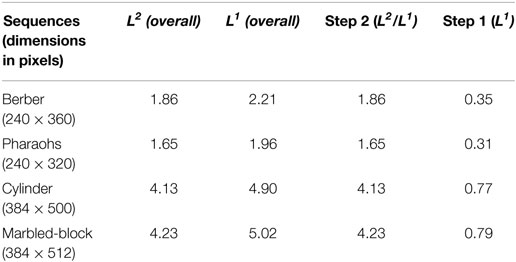
Table 1. Computation times per iteration (in seconds).

Table 1 reports the computation (CPU) times for both L¹ and L² regularizations, in the case of four different test images of different sizes. Columns 2 and 3 contain the overall CPU times. The third column gives the CPU time for the block-wise SVD updates solving a large-scale sparse system. These SVD computations occur in both L² and L¹ formulations (Step 2). The last column reports the CPU times for the pointwise updates in equation (8). These updates appear only in the L¹ formulation (Step 1). The simulations were run on an Intel i7-4500U Processor (4M Cache, up to 3.00 GHz), using MATLAB (2014b version).

4. Partial Derivatives

In computer vision, image derivatives are often approximated by locally averaged finite differences to lessen the impact of noise (Horn and Schunk, 1981; Marshall, 2005; Periaswamy and Farid, 2006; Sun et al., 2010; Heinrich et al., 2012; Mitiche et al., 2015). However, such fixed-support low-pass filtering does not generally fit the noise profile and can, therefore, be ineffective. A more effective way is to state differentiation as a spatially regularized variational problem, as was done in Mitiche et al. (2015). The process advocated in Mitiche et al. (2015) looked at the derivative of an image as a function which, when integrated, gives the image function. Consequently, the objective functional contained an anti-differentiation data term, which evaluates the conformity of a derivative to the image by constraining the integration of this derivative to produce the image. The functional also contained an L² regularization term. In this paper, we investigate a generalization, which accounts for derivative discontinuities using an L¹ regularization term because L² regularization constrains the image derivatives to be smooth everywhere and, as a result, would adversely blur their boundaries.

4.1. L¹ Regularized Differentiation

The partial derivatives I_x and I_y of an image will be estimated using an anti-differentiation characterization. The method for I_x will be explained in this section. The derivative I_y is computed by the same scheme applied to the transposed image. Since only two images are available along the time axis, the temporal derivative will be estimated using the Horn and Schunck definition of the temporal derivative (Horn and Schunk, 1981). Let f designate an approximation of the derivative. Recall that in Mitiche et al. (2015), the derivative was computed by minimizing the following functional with respect to f :

$E\left(f\right)=\frac{1}{2}{\int }_{\mathrm{\Omega }}\left(\mathrm{\parallel }\mathit{Df}-I{\mathrm{\parallel }}^2+\gamma \mathrm{\parallel }\mathit{\nabla f}{\mathrm{\parallel }}^2\right)\mathit{dxdy},$ (13)

where D is the anti-differentiation operator, γ is a positive constant, and ▽_f is the spatial gradient of f. The integral operator of anti-differentiation D is defined by

$\mathit{Df}\left(x,y\right)={\int }_0^{x}f\left(z,y\right)\mathit{dz}$ (14)

To generalize this formulation to preserve boundaries, we will replace the L² regularization term in equation (13) by an L¹ term: ${\int }_{\mathrm{\Omega }}{\left(f_x^2+f_y^2\right)}^{\frac{1}{2}}\mathit{dxdy}$. The objective functional becomes

$E\left(f\right)=\frac{1}{2}{\int }_{\mathrm{\Omega }}\left(\mathrm{\parallel }\mathit{Df}-I{\parallel }^2+\gamma {\int }_{\mathrm{\Omega }}{\left(f_x^2+f_y^2\right)}^{\frac{1}{2}}\right)\mathit{dxdy},$ (15)

The corresponding Euler–Lagrange equations are

$D^{\ast }\left(\mathit{Df}-I\right)-\gamma \frac{\partial }{\mathit{\partial x}}\frac{f_x}{{\left(f_x^2+f_y^2\right)}^{\frac{1}{2}}}-\gamma \frac{\partial }{\mathit{\partial y}}\frac{f_y}{{\left(f_x^2+f_y^2\right)}^{\frac{1}{2}}}=0,$ (16)

where D* is the adjoint operator of D given by, assuming Ω = [0,l] × [0,l], $D^{\ast }f\left(x,y\right)={\int }_x^{l}f\left(z,y\right)\mathit{dz}$.

Non-linearity occurs in the regularization terms of equation (23). As done in the previous section, we can, in practice, and without affecting in any significant way subsequent processing, extend differentiability to the origin by replacing the denominators by ${\left(f_x^2+f_y^2+\epsilon \right)}^{\frac{1}{2}}$, for some small positive ε. Also, and as we have done in the previous section, solve equation (16) iteratively, by evaluating, at each iteration k, the non-linear terms at the preceding iteration k − 1. More precisely, we have, after initialization, the following equation at iteration k:

$D^{\ast }\left({\mathit{Df}}^k-I\right)-\frac{\gamma }{{\left({\left(f_x^{k-1}\right)}^2+{\left(f_y^{k-1}\right)}^2+\epsilon \right)}^{\frac{1}{2}}}{\nabla }^2{f}^k=0$ (17)

As in Mitiche et al. (2015), discretization of equation (17) yields a large-scale sparse system of linear equations which can be solved by the Gauss–Seidel method.

4.2. Example

We apply the scheme to compute the derivatives of the noisy (Gaussian white noise, SNR = 1) synthetic chessboard image of Figure 2, which illustrates that L¹ regularized differentiation outperforms both the local finite-difference definition and L² regularized differentiation. A quantitative evaluation can be done by computing the MSE (mean squared error) and the SDE (standard deviation of error). Table 2 lists the results. Derivatives are in gray level (0–255 range) per pixel. The top part of the table gives the measurements as obtained from the whole image. The values listed in the bottom part of the table come from the vicinity of the image boundaries, using a 5 × 5 window centered on these. The results confirm visual inspection, i.e., that L¹ regularization outperforms both L² regularization and local finite differences.

FIGURE 2

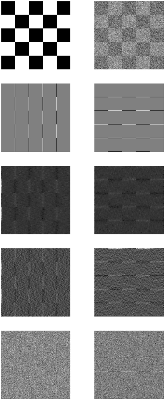
Figure 2. Noised chessboard. First row, chessboard image on the left and noised chessboard image on the right (SNR = 1). Second row, ground truth of partial derivatives: I_x on the left and I_y on the right. Third row, estimated partial derivatives using TV regularized differentiation with γ = 1: I_x on the left and I_y on the right. Fourth row, estimated partial derivative using L² regularized differentiation with γ = 1: I_x on the left I_y on the right. Fifth row, estimated partial derivative using forward difference of Horn and Schunck: I_x on the left and I_y on the right.

TABLE 2

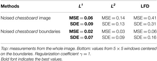
Table 2. Differentiation: L¹ regularization, L² regularization, and local finite differences (LFD) applied to noised chessboard image (SNR = 1) and evaluated using mean squared error (MSE) and standard deviation error (SDE).

5. Experimental Results

In this section, we expose various experiments showing the application of the described method to synthetic and real image sequences. In addition to displaying various experimental examples, we present a comparative and quantitative analysis that highlights the positive effects of L¹ regularization over the whole image domain, and particularly within motion boundaries. In our experiments, all formulation parameters are determined empirically and distances are measured in pixels. In all the examples, regularized differentiation’s coefficient γ has been fixed equal to 1. As approximated in Sekkati and Mitiche (2007), the focal length of the camera is 600 pixels. The position of the frontoparallel plane Z₀ is fixed to 6 × 10⁴ pixels. The initial values of scene flow and depth at each point are set to, respectively, 0 and Z₀. Coefficients α and β vary from a sequence to another and are given in the caption of each example.

5.1. Examples

Four image sequences with different characteristics served as samples to test the validity of our scheme and its implementation. Our displays include

• Anaglyphs, which provide a convenient way for subjective appraisal of the recovered object depth. When viewed with chromatic (red–cyan) glasses on good-quality photographic paper or on standard screens, anaglyphs give viewers a strong sense of depth. They are produced from one of the two input images and the computed depth map and are generally better perceived with full color resolution;

• Standard displays using color-coded depth so as to highlight image-depth variations;

• 3D reconstructed objects;

• 3D scene flow vector fields; and

• 2D optical flow fields corresponding to our recovered scene flow. This can serve as an indirect validation of our implementation when the 2D outputs are compared to standard optical flow methods (e.g., the well tested/researched benchmark algorithm of Horn and Schunck).

We provide several figures, each corresponding to an example and organized as follows. The first row includes (from left to right): (a) an anaglyph of the scene structure reconstructed from our method’s output and the first frame of the sequence; (b) a color-coded display of the recovered depth and the used color palette, with depth increasing from bottom (red) to top (purple); and (c) novel viewpoint images of the moving objects in the scene. The second row depicts (from left to right): (a) a view of the obtained scene flow; (b) a projected optical flow corresponding to our estimated scene flow; and (c) optical flow computed directly by the Horn and Schunck algorithm.

The following describes the four image sequences that we used:

• The Marbled-block synthetic image sequence (Figure 3) is taken from the database of KOGS/IAKS Laboratory, Germany. This sequence shows three blocks, two of them are moving. The rightmost block is moving backward to the left, whereas the front-most (smallest) block moves forward to the left. Some aspects of this sequence make its 3D interpretation challenging: the blocks and the floor have a similar macrotexture with weak spatiotemporal intensity variations within the textons. This makes the occluding boundaries of the blocks ill defined at some places. Also, the source of light position with respect to the blocks causes shadows, which move with the blocks.

• The Cylinder and box real sequence (Figure 4), provided in Debrunner and Ahuja (1998), depicts two moving objects, along with a moving background: a cylindrical surface rotating at a velocity of 1° per frame about the vertical axis and moving laterally at an image rate of about 0.15 pixel per frame toward the right, as well as a box translating at approximately 0.30 pixel per frame toward the right. Also, the background is translating to the right (parallel to the box motion) at a rate of about 0.15 pixel per frame. Those motions make 3D interpretation and recovery challenging in this example.

• The Berber real sequence (Figure 5) exhibits a sculpture rotating about the vertical axis and translating forward to the left in a static environment.

• The Pharaohs sequence (Figure 6) shows two moving sculptures in a static environment. The first (leftmost) figurine translates left and forward, whereas the second rotates about a nearly vertical axis to the right.

FIGURE 3

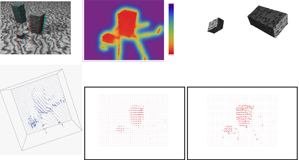
Figure 3. Marbled blocks sequence results (better perceived when figures are enlarged on screen). Parameters: α = 6 × 10⁷ and β = 10³. First row from left to right: an anaglyph of the structure reconstructed from the method’s output and the first frame of the sequence; a color-coded display of the recovered depth along with the used color palette, with depth increasing from bottom (red) to top (purple); novel viewpoint images of the two moving blocks. Second row: a view of the scene flow vectors; optical flow corresponding to the estimated scene flow; optical flow computed directly by the Horn and Schunck algorithm.

FIGURE 4

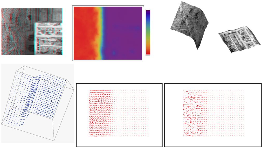
Figure 4. Cylinder and box sequence results (better perceived when figures are enlarged on screen). Parameters: α = 6 × 10⁷ and β = 10⁵. First row from left to right: an anaglyph of the structure reconstructed from the method’s output and the first frame of the sequence; a color-coded display of the recovered depth along with the used color palette, with depth increasing from bottom (red) to top (purple); novel viewpoint images of the cylindrical surface and the box. Second row: a view of the scene flow vectors; optical flow corresponding to the estimated scene flow; optical flow computed by the Horn and Schunck algorithm.

FIGURE 5

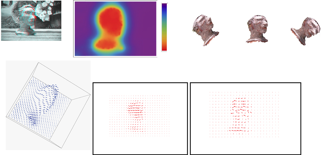
Figure 5. Berber figurine sequence results (better perceived when figures are enlarged on the screen). Parameters: α = 6 × 10⁸; β = 5 × 10⁵. First row from left to right: an anaglyph of the structure reconstructed from the method’s output and the first frame of the input image sequence; a color-coded display of the recovered depth along with the used color palette, with depth increasing from bottom (red) to top (purple); novel viewpoint images of the figurine. Second row: a view of the scene flow vectors; optical flow corresponding to the estimated scene flow; optical flow computed by the Horn and Schunck algorithm.

FIGURE 6

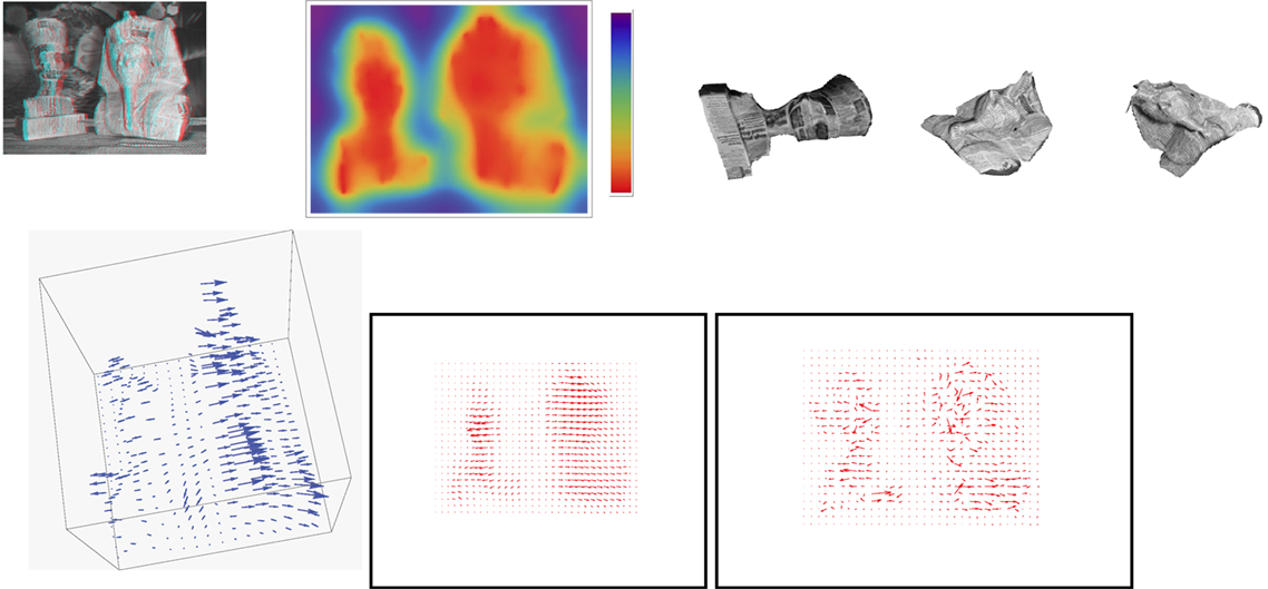
Figure 6. Pharaohs figurines sequence (better perceived when figures are enlarged on screen). Parameters: α = 6 × 10⁸; β = × 10². First row from left to right: an anaglyph of the structure reconstructed from the method’s output and the first frame of the input image sequence; a color-coded display of the recovered depth along with the used color palette, with depth increasing from bottom (red) to top (purple); novel viewpoint images of the figurines. Second row: a view of the scene flow vectors; optical flow corresponding to the estimated scene flow; optical flow computed by the Horn and Schunck algorithm.

The examples above support the validity of our scheme and its implementation. The obtained anaglyphs, color-coded depths, and 3D object reconstructions are consistent with the actual structures of the scenes. The displays of the estimated 3D scene flow and the corresponding 2D optical flow are consistent with the real motion of the objects in scenes. Also, the optical flow derived from our scene flow estimation is in line with a direct optical flow computation by the standard Horn and Schunck algorithm. We notice that the obtained fields are more regular and present less noise than those computed directly with Horn and Schunck algorithm. This is mainly due to the use of 3D information and regularized differentiation.

5.2. Comparative Analysis

We report a comprehensive comparative analysis, which demonstrates the benefits of our L¹ formulations. In particular, we focus our evaluations on the boundaries of motions and objects, so as to illustrate the boundary-preserving effect of our L¹ methods.

We began our comparative analysis by the simple synthetic sequence Squares, which includes two images with known motions. This sequence depicts two overlapping squares in opposite motions, along with a moving background. The motions for these three elements are known: a translation of the rightmost square by (−1, −1) pixels in the downward-left direction, a translation of the leftmost square by (1, 1) pixels in the top-right direction, and downward translation of the background by (0, −1) pixels. To better test the performance of evaluated schemes, we added noise independently to the first and second image. Noise values are from a discretized, shifted, and truncated Gaussian in the interval between 0 and 100 gray levels, within an overall range of [0, 255]. The first row of Figure 7 displays the first (noised) image (left) and the vector-coded ground truth (right). The second row depicts the optical flows, the first (left) obtained from a projection of the L² regularized scene flow (Mitiche et al., 2015) and the second from our L¹ regularized scene flow. In both cases, we estimated image derivatives with a finite-difference regularization based on the standard Horn and Schunck definition (Horn and Schunk, 1981). We refer to these methods as L²HS (left) and L¹HS (right). In the third row, we repeated the same experiment using regularized image differentiation instead of the finite differences. On the left, we depict the result using L² regularization for both scene flow and image-derivative estimations (L²L²) whereas on the right, we show the result for L¹ (L¹L¹). The optical flows resulting from the four methods are consistent with their expected overall appearance. However, we see clearly a difference between the performances of those algorithms.

FIGURE 7

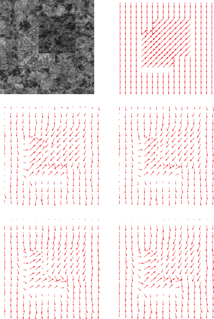
Figure 7. Squares synthetic sequence results. First row: the first (noised) image of the sequence (left) and the vector-coded ground truth (right). Second row: the optical flow corresponding to L²HS (left) and L¹HS (right). Third row: the optical flow corresponding to L²L² (left) and L¹L¹ (right).

Visually, the L¹L¹ scheme yielded the closest match to the vector-coded ground truth. To support this quantitatively, we added an evaluation based on two standard error measures for optical flow (Baker et al., 2011): average angular error (aae) and endpoint error (epe); see Table 3. The (L¹L¹) scheme performed better than the other methods.

TABLE 3

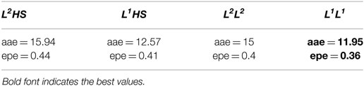
Table 3. Performance of L²HS, L¹HS, L²L², and L¹L¹ algorithms on the noised squares image (SNR = 1.12).

Figure 8 depicts another example for our comparative analysis. It uses the Hydrangea sequence of a real scene from the Middlebury data set (Baker et al., 2011). The sequence shows a rotating flower bouquet within a translating background, and the ground-truth flow of the sequence is given.¹ The first row of the figure displays the first of the two input images (left) and the vector-coded ground truth (right). The second row depicts the optical flows, the first (left) obtained from a projection of the L² regularized scene flow (Mitiche et al., 2015) and the second from our L¹ regularized scene flow. In both cases, we estimated image derivatives with a finite-difference regularization based on the standard Horn and Schunck definition (Horn and Schunk, 1981). We refer to these methods as L²HS (left) and L¹HS (right). In the third row, we repeated the same experiment using regularized image differentiation instead of the finite differences. On the left, we depict the result using L² regularization for both scene flow and image-derivative estimations (L²L²) whereas on the right, we show the result for L¹ (L¹L¹). Visually, the L¹L¹ scheme yielded the closest match to the vector-coded ground truth. Table 4 supports quantitatively these results. It reports two standard optical flow errors (aae and epe) (Baker et al., 2011), showing that the L¹L¹ scheme performed better than the other methods.

FIGURE 8

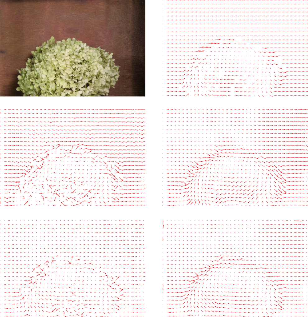
Figure 8. Hydrangea real sequence results. First row: the first image of the sequence (left) and the vector-coded ground truth (right). Second row: the optical flow corresponding to L²HS (left) and L¹HS (right). Third row: the optical flow corresponding to L²L² (left) and L¹L¹ (right).

TABLE 4

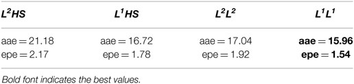
Table 4. Performance of L²HS, L¹HS, L²L², and L¹L¹ algorithms on the Hydrangea real sequence.

Figure 9 compares visually the results of L¹L¹ (proposed method) and L²L² (Mitiche et al., 2015) using the different examples in Section 1. The first column depicts the results of the proposed L¹L¹ method, whereas the second shows the results of Mitiche et al. (2015) (L²L²). The first row shows anaglyphs, the second color-coded depth, and the third 3D object reconstructions. The last two rows displayed both 3D scene flow and projected 2D optical flow fields. We can see that the results are better with L¹L¹ than with L²L²: the 3D parameters are better defined, clearer, and sharper, especially on the boundaries; flow fields are more regular and smooth.

FIGURE 9

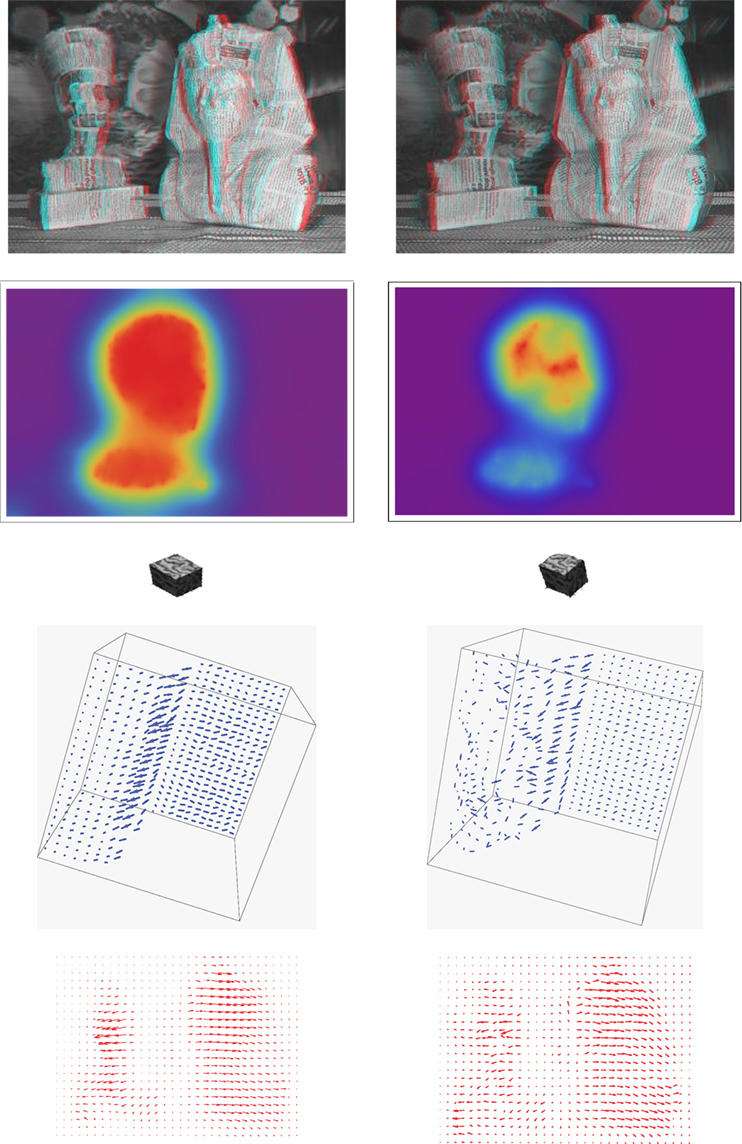
Figure 9. Visual inspection of the results of the proposed L¹L¹ method (first column) and the L²L² method in Mitiche et al. (2015) (second column). The first row shows anaglyphs, the second color-coded depth, and the third 3D object reconstructions. The last two rows depict 3D scene flow and projected 2D optical flow fields.

Tables 5 and 6 report quantitative comparisons of the four algorithms (L²HS and L¹HS in Table 5; L²L² and L¹L¹ in Table 6) using three standard error measures (Baker et al., 2011): average angular error (aae), standard angular error (stae), and endpoint error (epe). Errors are computed between the motion resulting from scene flow and the optical flow ground truth. As we do not have scene flow ground truth for these real examples, evaluations of the resulting (projected) optical flow are a good indirect way to assess scene flow results. We constructed an optical flow ground truth using SURF-based (Bay et al., 2008) detection and correspondences of the key points in the two images. Then, the velocity coordinates of these key points are computed, yielding an optical flow ground truth. Tables 5 and 6 confirm that the use of our L¹ regularization improves the results and that the L¹L¹ formulation outperforms the other methods.

TABLE 5

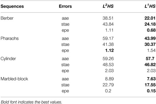
Table 5. Errors for the L²HS and L¹HS formulations.

TABLE 6

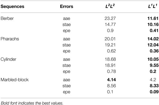
Table 6. Errors for the L²L² and L¹L¹ formulations.

In the following part of our comparative analysis, we will focus on the assessment (both qualitative and quantitative) of motion within objects boundaries, as preserving these is an important feature of our L¹ formulation.

Let us start with a qualitative visual inspection by displaying the images of the gradient of motion for each of the four methods (L²HS, L¹HS, L²L², and L¹L¹); see Figure 10. We note that with our L¹ regularization, points on the boundaries of motion are brighter (sharper). This is due to the fact that our L¹ formulation preserves sharp boundaries.

FIGURE 10

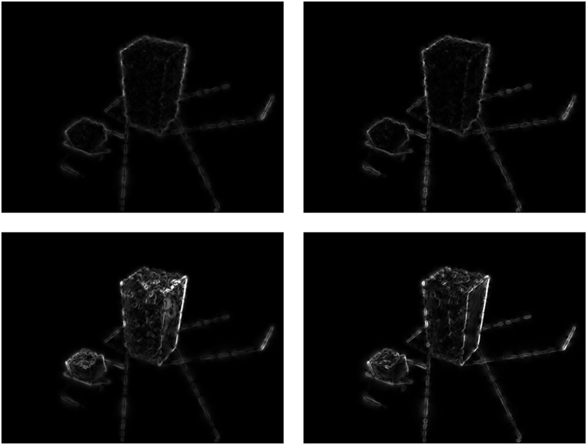
Figure 10. Gradients of optical flow for the Marbled blocks sequence. First row: L²HS (left) and L¹HS (right). Second row: L²L² (left) and L¹L¹ (right).

To support these results, we added quantitative evaluations based on aae, stae, and epe errors: Table 7 reports the results for L²HS and L¹HS; Table 8 reports the results for L²L² and L¹L¹. Errors are computed between the motion projected from the obtained scene flow and the optical flow ground truth within 7 × 7 windows centered at a set of key points on motion boundaries (the key points are those for which we have motion ground truth). Tables 7 and 8 report the results, which clearly indicate that our L¹L¹ formulation outperforms all the other methods.

TABLE 7

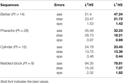
Table 7. Quantitative evaluations on the boundaries of motion (L²HS and L¹HS).

TABLE 8

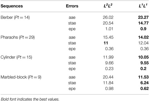
Table 8. Quantitative evaluations on the boundaries of motion (L²L² and L¹L¹).

6. Conclusion

This study investigated a boundary-preserving method for joint recovery of scene flow and relative depth from a monocular sequence of images. The scheme built upon the basic formulation of Mitiche et al. (2015). It minimized a functional composed of the data conformity term of Mitiche et al. (2015), which relates the image sequence spatiotemporal variations to scene flow and depth, and an L¹ regularization term, rather than L² as in Mitiche et al. (2015). Therefore, this afforded a boundary-preserving version of the basic formulation. The corresponding non-linear Euler–Lagrange equations were discretized and solved iteratively by a scheme, which solved at each iteration a large-scale sparse system of linear equations in the unknowns of scene flow and depth. The image derivatives were estimated by a variational method with L¹ regularization. This also led to an iterative method of resolution, which consisted of solving a large sparse system of linear equations at each iteration. Experiments show that the scheme is sound and efficient. The examples demonstrated the need to regularize scene flow and depth so as to take into account their boundaries, i.e., sharp spatial transitions of scene flow or depth. The results justify extensive further investigations, particularly concerning quantitative, i.e., ground truth controlled evaluation, motion of large extent, and image noise and resolution in common practical settings.

The choice of a continuous alternating optimization scheme for our problem can be motivated by two important facts. First, we are dealing with continuous variables, and therefore, a continuous (not discrete) Euler–Lagrange regularization approach is a natural choice. Furthermore, our alternating scheme for solving the ensuing non-linear Euler–Lagrange equations has a computational complexity that behaves linearly w.r.t the number of grid points (N). This is important in practice, particularly when dealing with large image sequences. Of course, it would be very interesting to investigate other regularization options for estimating scene flow and depth from a single image sequence, for instance:

• Discrete Markov Random Fields (MRFs): MRFs were previously investigated for optical flow using sub-modular pairwise potentials (Lempitsky et al., 2008). MRF models can benefit from powerful combinatorial optimization techniques such as graph cuts (Boykov et al., 2001). It is worth noting, however, that adapting discrete MRFs to our continuous setting requires some technical care and is not straightforward.

• Regularization based on non-local means filtering (Favaro, 2010). Non-local means can preserve edges and textures. They were applied successfully to thin structures in depth-from-defocus problems (Favaro, 2010).

• State-of-the-art solvers for non-smooth problems such as the primal-dual algorithm of Chambolle and Pock (2011).

Author Contributions

Ms. YM is a PhD student at INRS under the supervision of Prof. AM. Dr. IA is a professor at École de Technologie Supérieure, Montreal, and co-supervisor of YM. The authors have all contributed, to varying degrees, to the theoretical/methodological/experimental aspects of this paper.

Conflict of Interest Statement

The authors declare that the research was conducted in the absence of any commercial or financial relationships that could be construed as a potential conflict of interest.

Footnote

1. ^http://vision.middlebury.edu/flow/

References

Aubert, G., Deriche, R., and Kornprobst, P. (1999). Computing optical flow via variational techniques. SIAM J. Appl. Math. 60, 156–182. doi: 10.1137/S0036139998340170

CrossRef Full Text | Google Scholar

Aubert, G., and Kornprobst, P. (2002). Mathematical Problems in Image Processing. Springer.

Google Scholar

Baker, S., Scharstein, D., Lewis, J. P., Roth, S., Black, M. J., and Szeliski, R. (2011). A database and evaluation methodology for optical flow. Int. J. Comput. Vis. 92, 1–31. doi:10.1007/s11263-010-0390-2

CrossRef Full Text | Google Scholar

Bay, H., Ess, A., Tuytelaars, T., and Van Gool, L. (2008). Speeded-up robust features (surf). Comput. Vision Image Understand. 110, 346–359. doi:10.1016/j.cviu.2007.09.014

CrossRef Full Text | Google Scholar

Boykov, Y., Veksler, O., and Zabih, R. (2001). Fast approximate energy minimization via graph cuts. IEEE Trans. Pattern Anal. Mach. Intell. 23, 1222–1239. doi:10.1109/34.969114

CrossRef Full Text | Google Scholar

Chambolle, A., and Pock, T. (2011). A first-order primal-dual algorithm for convex problems with applications to imaging. J. Math. Imag. Vision 40, 120–145. doi:10.1007/s10851-010-0251-1

CrossRef Full Text | Google Scholar

Ciarlet, P. (1994). Introduction a l’analyse numerique matricielle et a l’optimisation, 5th Edn. Masson.

Google Scholar

Debrunner, C., and Ahuja, N. (1998). Segmentation and factorization-based motion and structure estimation for long image sequences. IEEE Trans. Pattern Anal. Mach. Intell. 20, 206–211. doi:10.1109/34.659941

CrossRef Full Text | Google Scholar

Favaro, P. (2010). “Recovering thin structures via nonlocal-means regularization with application to depth from defocus,” in IEEE Conference on Computer Vision and Pattern Recognition (CVPR), 1133–1140.

Google Scholar

Forsythe, G., Malcolm, M., and Moler, C. (1977). Computer Methods for Mathematical Computations. Prentice-Hall.

Google Scholar

Heinrich, M. P., Jenkinson, M., Bhushan, M., Matin, T., Gleeson, F. V., Brady, M., et al. (2012). Mind: modality independent neighbourhood descriptor for multi-modal deformable registration. Med. Image Anal. 16, 1423–1435. doi:10.1016/j.media.2012.05.008

PubMed Abstract | CrossRef Full Text | Google Scholar

Horn, B., and Schunk, B. (1981). Determining optical flow. Artif. Intell. 17, 185–203. doi:10.1016/0004-3702(81)90024-2

CrossRef Full Text | Google Scholar

Huguet, F., and Devernay, F. (2007). “A variational method for scene flow estimation from stereo sequences,” in 2007 IEEE 11th International Conference on Computer Vision (ICCV) (IEEE), 1–7.

Google Scholar

Lempitsky, V. S., Roth, S., and Rother, C. (2008). “FusionFlow: discrete-continuous optimization for optical flow estimation,” in IEEE Conference on Computer Vision and Pattern Recognition (CVPR), 1–8.

Google Scholar

Longuet-Higgins, H., and Prazdny, K. (1981). The interpretation of a moving retinal image. Proc. R. Soc. Lond. B 208, 385–397. doi:10.1098/rspb.1980.0057

CrossRef Full Text | Google Scholar

Marshall, S. (2005). Depth dependence of ambient noise. IEEE J. Oceanic Eng. 30, 275–281. doi:10.1109/JOE.2005.850876

CrossRef Full Text | Google Scholar

Mitiche, A., and Aggarwal, J. (2013). Computer Vision Analysis of Image Motion by Variational Methods. Springer.

Google Scholar

Mitiche, A., Mathlouthi, Y., and Ben Ayed, I. (2015). Monocular concurrent recovery of structure and motion scene flow. Front. ICT 2:16. doi:10.3389/fict

CrossRef Full Text | Google Scholar

Mitiche, A., and Sekkati, H. (2006). Optical flow 3D segmentation and interpretation: a variational method with active curve evolution and level sets. IEEE Trans. Pattern Anal. Mach. Intell. 28, 1818–1829. doi:10.1109/TPAMI.2006.232

PubMed Abstract | CrossRef Full Text | Google Scholar

Periaswamy, S., and Farid, H. (2006). Medical image registration with partial data. Med. Image Anal. 10, 452–464. doi:10.1016/j.media.2005.03.006

PubMed Abstract | CrossRef Full Text | Google Scholar

Pons, J.-P., Keriven, R., and Faugeras, O. (2007). Multi-view stereo reconstruction and scene flow estimation with a global image-based matching score. Int. J. Comput. Vis. 72, 179–193. doi:10.1007/s11263-006-8671-5

CrossRef Full Text | Google Scholar

Sekkati, H., and Mitiche, A. (2007). A variational method for the recovery of dense 3D structure from motion. J. Rob. Auton. Syst. 55, 597–607. doi:10.1016/j.robot.2006.11.006

CrossRef Full Text | Google Scholar

Stoer, J., and Bulirsch, R. (2002). Introduction to Numerical Analysis, Texts in Applied Mathematics, 3rd Edn, Vol. 12. New York: Springer.

Google Scholar

Sun, D., Roth, S., and Black, M. J. (2010). “Secrets of optical flow estimation and their principles,” in 2010 IEEE Conference on Computer Vision and Pattern Recognition (CVPR) (IEEE), 2432–2439.

Google Scholar

Vedula, S., Rander, P., Collins, R., and Kanade, T. (2005). Three-dimensional scene flow. IEEE Trans. Pattern Anal. Mach. Intell. 27, 475–480. doi:10.1109/TPAMI.2005.63

PubMed Abstract | CrossRef Full Text | Google Scholar

Vogel, C., Schindler, K., and Roth, S. (2013). “Piecewise rigid scene flow,” in IEEE International Conference on Computer Vision (ICCV).

Google Scholar

Vogel, C. R. (2002). Computational Methods for Inverse Problems. SIAM Frontiers in Applied Mathematics.

Google Scholar

Wedel, A., Rabe, C., Vaudrey, T., Brox, T., Franke, U., and Cremers, D. (2008). Efficient Dense Scene Flow from Sparse or Dense Stereo Data. Springer.

Google Scholar